From Wikipedia, the free encyclopedia
In quantum mechanics, bra–ket notation is a standard notation for describing quantum states, composed of angle brackets and vertical bars. It can also be used to denote abstract vectors and linear functionals in mathematics. It is so called because the inner product (or dot product on a complex vector space) of two states is denoted by
 called the bra /brɑː/, and a right part,
  , called the ket /kɛt/. The notation was introduced in 1939 by Paul Dirac[1] and is also known as Dirac notation, though the notation has precursors in Grassmann's use of the notation
 ![[\phi\mid\psi]](//upload.wikimedia.org/math/9/7/1/971f62ad54ee09d21680bbf9e8ef071b.png) for his inner products nearly 100 years earlier.[2][3]
for his inner products nearly 100 years earlier.[2][3]
Bra–ket notation is widespread in quantum mechanics: almost every phenomenon that is explained using quantum mechanics—including a large portion of modern physics — is usually explained with the help of bra-ket notation. Part of the appeal of the notation is the abstract representation-independence it encodes, together with its versatility in producing a specific representation (e.g. x, or p, or eigenfunction base) without much ado, or excessive reliance on the nature of the linear spaces involved. The overlap expression is typically interpreted as the probability amplitude for the state ψ to collapse into the state φ.
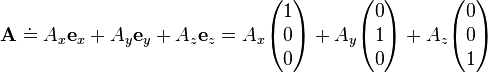
The vector A can be written using any set of basis vectors and corresponding coordinate system. Informally basis vectors are like "building blocks of a vector": they are added together to compose a vector, and the coordinates are the numerical coefficients of basis vectors in each direction. Two useful representations of a vector are simply a linear combination of basis vectors, and column matrices. Using the familiar Cartesian basis, a vector A may be written as

respectively, where ex, ey, ez denote the Cartesian basis vectors (all are orthogonal unit vectors) and Ax, Ay, Az are the corresponding coordinates, in the x, y, z directions. In a more general notation, for any basis in 3-d space one writes
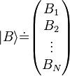
Even more generally, A can be a vector in a complex Hilbert space. Some Hilbert spaces, like ℂN, have finite dimension, while others have infinite dimension. In an infinite-dimensional space, the column-vector representation of A would be a list of infinitely many complex numbers.
 , Dirac's notation for a vector uses vertical bars and angular brackets:
  . When this notation is used, these vectors are called "ket", read as "ket-A".[4] This applies to all vectors, the resultant vector and the basis. The previous vectors are now written
" has a specific and universal mathematical meaning, while just the "A" by itself does not. Nevertheless, for convenience, there is usually some logical scheme behind the labels inside kets, such as the common practice of labeling energy eigenkets in quantum mechanics through a listing of their quantum numbers. Further note that a ket and its representation by a coordinate vector are not the same mathematical object: a ket does not require specification of a basis, whereas the coordinate vector needs a basis in order to be well defined (the same holds for an operator and its representation by a matrix).[5] In this context, one should best use a symbol different than the equal sign, for example the symbol ≐ , read as "is represented by".
 denotes the complex conjugate of Ai. A special case is the inner product of a vector with itself, which is the square of its norm (magnitude):
The purpose of "splitting" the inner product into a bra and a ket is that both the bra ⟨A| and the ket |B⟩ are meaningful on their own, and can be used in other contexts besides within an inner product. There are two main ways to think about the meanings of separate bras and kets:
The conjugate transpose (also called Hermitian conjugate) of a bra is the corresponding ket and vice versa:
In mathematics terminology, the vector space of bras is the dual space to the vector space of kets, and corresponding bras and kets are related by the Riesz representation theorem.
In quantum mechanics, it is common practice to write down kets which have infinite norm, i.e. non-normalisable wavefunctions. Examples include states whose wavefunctions are Dirac delta functions or infinite plane waves. These do not, technically, belong to the Hilbert space itself. However, the definition of "Hilbert space" can be broadened to accommodate these states (see the Gelfand–Naimark–Segal construction or rigged Hilbert spaces). The bra-ket notation continues to work in an analogous way in this broader context.
For a rigorous treatment of the Dirac inner product of non-normalizable states, see the definition given by D. Carfì.[6][7] For a rigorous definition of basis with a continuous set of indices and consequently for a rigorous definition of position and momentum basis, see.[8] For a rigorous statement of the expansion of an S-diagonalizable operator, or observable, in its eigenbasis or in another basis, see.[9]
Banach spaces are a different generalization of Hilbert spaces. In a Banach space B, the vectors may be notated by kets and the continuous linear functionals by bras. Over any vector space without topology, we may also notate the vectors by kets and the linear functionals by bras. In these more general contexts, the bracket does not have the meaning of an inner product, because the Riesz representation theorem does not apply.


The Hilbert space of a spin-0 point particle is spanned by a "position basis" { |r⟩ }, where the label r extends over the set of all points in position space. Since there are uncountably infinitely many vectors in the basis, this is an uncountably infinite-dimensional Hilbert space. The dimensions of the Hilbert space (usually infinite) and position space (usually 1, 2 or 3) are not to be conflated.
Starting from any ket |Ψ⟩ in this Hilbert space, we can define a complex scalar function of r, known as a wavefunction:
It is then customary to define linear operators acting on wavefunctions in terms of linear operators acting on kets, by
 is the state with a definite value of the spin operator Sz equal to +1/2 and
  is the state with a definite value of the spin operator Sz equal to −1/2.
Since these are a basis, any quantum state of the particle can be expressed as a linear combination (i.e., quantum superposition) of these two states:
A different basis for the same Hilbert space is:
Again, any state of the particle can be expressed as a linear combination of these two:
There is a mathematical relationship between aψ, bψ, cψ, dψ; see change of basis.
It is common among physicists to use the same symbol for labels and constants in the same equation. It supposedly becomes easier to identify that the constant is related to the labeled object, and is claimed that the divergent nature of each will eliminate any ambiguity and no further differentiation is required. For example, α̂ |α⟩ = α|α⟩, where the symbol α is used simultaneously as the name of the operator α̂, its eigenvector |α⟩ and the associated eigenvalue α.
Something similar occurs in component notation of vectors. While Ψ (uppercase) is traditionally associated with wavefunctions, ψ (lowercase) may be used to denote a label, a wave function or complex constant in the same context, usually differentiated only by a subscript.
The main abuses are including operations inside the vector labels. This is usually done for a fast notation of scaling vectors. E.g. if the vector |α⟩ is scaled by √2, it might be denoted by |α/√2⟩, which makes no sense since α is a label, not a function or a number, so you can't perform operations on it.
This is especially common when denoting vectors as tensor products, where part of the labels are moved outside the designed slot. E.g. |α⟩ = |α/√2⟩1 ⊗ |α/√2⟩2. Here part of the labeling that should state that all three vectors are different was moved outside the kets, as subscripts 1 and 2. And a further abuse occurs, since α is meant to refer to the norm of the first vector – which is a label is denoting a value.
In an N-dimensional Hilbert space, |ψ⟩ can be written as an N×1 column vector, and then A is an N×N matrix with complex entries. The ket A|ψ⟩ can be computed by normal matrix multiplication.
Linear operators are ubiquitous in the theory of quantum mechanics. For example, observable physical quantities are represented by self-adjoint operators, such as energy or momentum, whereas transformative processes are represented by unitary linear operators such as rotation or the progression of time.
If the same state vector appears on both bra and ket side,
One of the uses of the outer product is to construct projection operators. Given a ket |ψ⟩ of norm 1, the orthogonal projection onto the subspace spanned by |ψ⟩ is
Self-adjoint operators, where A = A†, play an important role in quantum mechanics; for example, an observable is always described by a self-adjoint operator. If A is a self-adjoint operator, then ⟨ψ|A|ψ⟩ is always a real number (not complex). This implies that expectation values of observables are real.
If |ψ⟩ is a ket in V and |φ⟩ is a ket in W, the direct product of the two kets is a ket in V ⊗ W. This is written in various notations:
 , for a Hilbert space H, with respect to the norm from an inner product
  . From basic functional analysis we know that any ket |ψ⟩ can also be written as
 the inner product on the Hilbert space.
From the commutativity of kets with (complex) scalars now follows that
In quantum mechanics, it often occurs that little or no information about the inner product of two arbitrary (state) kets is present, while it is still possible to say something about the expansion coefficients
  and
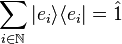
and  of those vectors with respect to a specific (orthonormalized) basis. In this case, it is particularly useful to insert the unit operator into the bracket one time or more.
Let be a Hilbert space and
  is a vector in . What physicists would denote as |h⟩ is the vector itself. That is
 be the dual space of . This is the space of linear functionals on . The isomorphism
  is defined by
  where for all
  we have
 and are just different notations for expressing an inner product between two elements in a Hilbert space (or for the first three, in any inner product space). Notational confusion arises when identifying
  and
and  with
with  and
and  respectively. This is because of literal symbolic substitutions. Let
  and let
  . This gives
Moreover, mathematicians usually write the dual entity not at the first place, as the physicists do, but at the second one, and they don't use the *-symbol, but an overline (which the physicists reserve for averages and Dirac conjugation) to denote conjugate-complex numbers, i.e. for scalar products mathematicians usually write
- ,
 called the bra /brɑː/, and a right part,
  , called the ket /kɛt/. The notation was introduced in 1939 by Paul Dirac[1] and is also known as Dirac notation, though the notation has precursors in Grassmann's use of the notation
 ![[\phi\mid\psi]](http://upload.wikimedia.org/math/9/7/1/971f62ad54ee09d21680bbf9e8ef071b.png) for his inner products nearly 100 years earlier.[2][3]
for his inner products nearly 100 years earlier.[2][3]Bra–ket notation is widespread in quantum mechanics: almost every phenomenon that is explained using quantum mechanics—including a large portion of modern physics — is usually explained with the help of bra-ket notation. Part of the appeal of the notation is the abstract representation-independence it encodes, together with its versatility in producing a specific representation (e.g. x, or p, or eigenfunction base) without much ado, or excessive reliance on the nature of the linear spaces involved. The overlap expression
 is typically interpreted as the probability amplitude for the state ψ to collapse into the state φ.
Vector spaces
Background: Vector spaces
In physics, basis vectors allow any Euclidean vector to be represented geometrically using angles and lengths, in different directions, i.e. in terms of the spatial orientations. It is simpler to see the notational equivalences between ordinary notation and bra-ket notation; so, for now, consider a vector A starting at the origin and ending at an element of 3-d Euclidean space; the vector then is specified by this end-point, a triplet of elements in the field of real numbers, symbolically dubbed as A ∈ ℝ3.The vector A can be written using any set of basis vectors and corresponding coordinate system. Informally basis vectors are like "building blocks of a vector": they are added together to compose a vector, and the coordinates are the numerical coefficients of basis vectors in each direction. Two useful representations of a vector are simply a linear combination of basis vectors, and column matrices. Using the familiar Cartesian basis, a vector A may be written as


3d real vector components and bases projection; similarities between vector calculus notation and Dirac notation. Projection is an important feature of the Dirac notation.
respectively, where ex, ey, ez denote the Cartesian basis vectors (all are orthogonal unit vectors) and Ax, Ay, Az are the corresponding coordinates, in the x, y, z directions. In a more general notation, for any basis in 3-d space one writes


Even more generally, A can be a vector in a complex Hilbert space. Some Hilbert spaces, like ℂN, have finite dimension, while others have infinite dimension. In an infinite-dimensional space, the column-vector representation of A would be a list of infinitely many complex numbers.
Ket notation for vectors
Rather than boldtype, over arrows, underscores etc. conventionally used elsewhere, , Dirac's notation for a vector uses vertical bars and angular brackets:
  . When this notation is used, these vectors are called "ket", read as "ket-A".[4] This applies to all vectors, the resultant vector and the basis. The previous vectors are now written

 " has a specific and universal mathematical meaning, while just the "A" by itself does not. Nevertheless, for convenience, there is usually some logical scheme behind the labels inside kets, such as the common practice of labeling energy eigenkets in quantum mechanics through a listing of their quantum numbers. Further note that a ket and its representation by a coordinate vector are not the same mathematical object: a ket does not require specification of a basis, whereas the coordinate vector needs a basis in order to be well defined (the same holds for an operator and its representation by a matrix).[5] In this context, one should best use a symbol different than the equal sign, for example the symbol ≐ , read as "is represented by".
Inner products and bras
An inner product is a generalization of the dot product. The inner product of two vectors is a scalar. bra-ket notation uses a specific notation for inner products:

 denotes the complex conjugate of Ai. A special case is the inner product of a vector with itself, which is the square of its norm (magnitude):

The purpose of "splitting" the inner product into a bra and a ket is that both the bra ⟨A| and the ket |B⟩ are meaningful on their own, and can be used in other contexts besides within an inner product. There are two main ways to think about the meanings of separate bras and kets:
Bras and kets as row and column vectors
For a finite-dimensional vector space, using a fixed orthonormal basis, the inner product can be written as a matrix multiplication of a row vector with a column vector:

The conjugate transpose (also called Hermitian conjugate) of a bra is the corresponding ket and vice versa:


Bras as linear operators on kets
A more abstract definition, which is equivalent but more easily generalized to infinite-dimensional spaces, is to say that bras are linear functionals on kets, i.e. operators that input a ket and output a complex number. The bra operators are defined to be consistent with the inner product.In mathematics terminology, the vector space of bras is the dual space to the vector space of kets, and corresponding bras and kets are related by the Riesz representation theorem.
Non-normalizable states and non-Hilbert spaces
bra-ket notation can be used even if the vector space is not a Hilbert space.In quantum mechanics, it is common practice to write down kets which have infinite norm, i.e. non-normalisable wavefunctions. Examples include states whose wavefunctions are Dirac delta functions or infinite plane waves. These do not, technically, belong to the Hilbert space itself. However, the definition of "Hilbert space" can be broadened to accommodate these states (see the Gelfand–Naimark–Segal construction or rigged Hilbert spaces). The bra-ket notation continues to work in an analogous way in this broader context.
For a rigorous treatment of the Dirac inner product of non-normalizable states, see the definition given by D. Carfì.[6][7] For a rigorous definition of basis with a continuous set of indices and consequently for a rigorous definition of position and momentum basis, see.[8] For a rigorous statement of the expansion of an S-diagonalizable operator, or observable, in its eigenbasis or in another basis, see.[9]
Banach spaces are a different generalization of Hilbert spaces. In a Banach space B, the vectors may be notated by kets and the continuous linear functionals by bras. Over any vector space without topology, we may also notate the vectors by kets and the linear functionals by bras. In these more general contexts, the bracket does not have the meaning of an inner product, because the Riesz representation theorem does not apply.
Usage in quantum mechanics
The mathematical structure of quantum mechanics is based in large part on linear algebra:- Wave functions and other quantum states can be represented as vectors in a complex Hilbert space. (The exact structure of this Hilbert space depends on the situation.) In bra-ket notation, for example, an electron might be in the "state" |ψ⟩. (Technically, the quantum states are rays of vectors in the Hilbert space, as c|ψ⟩ corresponds to the same state for any nonzero complex number c.)
- Quantum superpositions can be described as vector sums of the constituent states. For example, an electron in the state |1⟩ + i |2⟩ is in a quantum superposition of the states |1⟩ and |2⟩.
- Measurements are associated with linear operators (called observables) on the Hilbert space of quantum states.
- Dynamics are also described by linear operators on the Hilbert space. For example, in the Schrödinger picture, there is a linear time evolution operator U with the property that if an electron is in state |ψ⟩ right now, then in one second it will be in the state U|ψ⟩, the same U for every possible |ψ⟩.
- Wave function normalization is scaling a wave function so that its norm is 1.
Spinless position–space wave function

Discrete components Ak of a complex vector |A⟩ = ∑k Ak|ek⟩, which belongs to a countably infinite-dimensional Hilbert space; there are countably infinitely many k values and basis vectors |ek⟩.

Continuous components ψ(x) of a complex vector |ψ⟩ = ∫ dx ψ(x)|x⟩, which belongs to an uncountably infinite-dimensional Hilbert space; there are infinitely many x values and basis vectors |x⟩.
Components of complex vectors plotted against index number; discrete k and continuous x. Two particular components out of infinitely many are highlighted.
The Hilbert space of a spin-0 point particle is spanned by a "position basis" { |r⟩ }, where the label r extends over the set of all points in position space. Since there are uncountably infinitely many vectors in the basis, this is an uncountably infinite-dimensional Hilbert space. The dimensions of the Hilbert space (usually infinite) and position space (usually 1, 2 or 3) are not to be conflated.
Starting from any ket |Ψ⟩ in this Hilbert space, we can define a complex scalar function of r, known as a wavefunction:
 .
.
 .
.It is then customary to define linear operators acting on wavefunctions in terms of linear operators acting on kets, by


Overlap of states
In quantum mechanics the expression ⟨φ|ψ⟩ is typically interpreted as the probability amplitude for the state ψ to collapse into the state φ. Mathematically, this means the coefficient for the projection of ψ onto φ. It is also described as the projection of state ψ onto state φ.Changing basis for a spin-1/2 particle
A stationary spin-½ particle has a two-dimensional Hilbert space. One orthonormal basis is:
 is the state with a definite value of the spin operator Sz equal to +1/2 and
  is the state with a definite value of the spin operator Sz equal to −1/2.
Since these are a basis, any quantum state of the particle can be expressed as a linear combination (i.e., quantum superposition) of these two states:

A different basis for the same Hilbert space is:

Again, any state of the particle can be expressed as a linear combination of these two:


There is a mathematical relationship between aψ, bψ, cψ, dψ; see change of basis.
Misleading uses
There are a few conventions and abuses of notation that are generally accepted by the physics community, but which might confuse the non-initiated.It is common among physicists to use the same symbol for labels and constants in the same equation. It supposedly becomes easier to identify that the constant is related to the labeled object, and is claimed that the divergent nature of each will eliminate any ambiguity and no further differentiation is required. For example, α̂ |α⟩ = α|α⟩, where the symbol α is used simultaneously as the name of the operator α̂, its eigenvector |α⟩ and the associated eigenvalue α.
Something similar occurs in component notation of vectors. While Ψ (uppercase) is traditionally associated with wavefunctions, ψ (lowercase) may be used to denote a label, a wave function or complex constant in the same context, usually differentiated only by a subscript.
The main abuses are including operations inside the vector labels. This is usually done for a fast notation of scaling vectors. E.g. if the vector |α⟩ is scaled by √2, it might be denoted by |α/√2⟩, which makes no sense since α is a label, not a function or a number, so you can't perform operations on it.
This is especially common when denoting vectors as tensor products, where part of the labels are moved outside the designed slot. E.g. |α⟩ = |α/√2⟩1 ⊗ |α/√2⟩2. Here part of the labeling that should state that all three vectors are different was moved outside the kets, as subscripts 1 and 2. And a further abuse occurs, since α is meant to refer to the norm of the first vector – which is a label is denoting a value.
Linear operators
Linear operators acting on kets
A linear operator is a map that inputs a ket and outputs a ket. (In order to be called "linear", it is required to have certain properties.) In other words, if A is a linear operator and |ψ⟩ is a ket, then A|ψ⟩ is another ket.In an N-dimensional Hilbert space, |ψ⟩ can be written as an N×1 column vector, and then A is an N×N matrix with complex entries. The ket A|ψ⟩ can be computed by normal matrix multiplication.
Linear operators are ubiquitous in the theory of quantum mechanics. For example, observable physical quantities are represented by self-adjoint operators, such as energy or momentum, whereas transformative processes are represented by unitary linear operators such as rotation or the progression of time.
Linear operators acting on bras
Operators can also be viewed as acting on bras from the right hand side. Specifically, if A is a linear operator and ⟨φ| is a bra, then ⟨φ|A is another bra defined by the rule
 .
.
 .
.If the same state vector appears on both bra and ket side,

Outer products
A convenient way to define linear operators on H is given by the outer product: if ⟨φ| is a bra and |ψ⟩ is a ket, the outer product
 .
.
 .
.
One of the uses of the outer product is to construct projection operators. Given a ket |ψ⟩ of norm 1, the orthogonal projection onto the subspace spanned by |ψ⟩ is

Hermitian conjugate operator
Just as kets and bras can be transformed into each other (making |ψ⟩ into ⟨ψ|), the element from the dual space corresponding to A|ψ⟩ is ⟨ψ|A†, where A† denotes the Hermitian conjugate (or adjoint) of the operator A. In other words, if and only if
  .
.
 if and only if
  .
.Self-adjoint operators, where A = A†, play an important role in quantum mechanics; for example, an observable is always described by a self-adjoint operator. If A is a self-adjoint operator, then ⟨ψ|A|ψ⟩ is always a real number (not complex). This implies that expectation values of observables are real.
Properties
bra-ket notation was designed to facilitate the formal manipulation of linear-algebraic expressions. Some of the properties that allow this manipulation are listed herein. In what follows, c1 and c2 denote arbitrary complex numbers, c∗ denotes the complex conjugate of c, A and B denote arbitrary linear operators, and these properties are to hold for any choice of bras and kets.Linearity[edit]
- Since bras are linear functionals,

- By the definition of addition and scalar multiplication of linear functionals in the dual space,[10]

Associativity
Given any expression involving complex numbers, bras, kets, inner products, outer products, and/or linear operators (but not addition), written in bra-ket notation, the parenthetical groupings do not matter (i.e., the associative property holds). For example:

Hermitian conjugation
bra-ket notation makes it particularly easy to compute the Hermitian conjugate (also called dagger, and denoted †) of expressions. The formal rules are:- The Hermitian conjugate of a bra is the corresponding ket, and vice versa.
- The Hermitian conjugate of a complex number is its complex conjugate.
- The Hermitian conjugate of the Hermitian conjugate of anything (linear operators, bras, kets, numbers) is itself—i.e.,
-
- (x†)† = x.
- Given any combination of complex numbers, bras, kets, inner products, outer products, and/or linear operators, written in bra-ket notation, its Hermitian conjugate can be computed by reversing the order of the components, and taking the Hermitian conjugate of each.
- Kets:

- Inner products:
- Matrix elements:


- Outer products:

Composite bras and kets
Two Hilbert spaces V and W may form a third space V ⊗ W by a tensor product. In quantum mechanics, this is used for describing composite systems. If a system is composed of two subsystems described in V and W respectively, then the Hilbert space of the entire system is the tensor product of the two spaces. (The exception to this is if the subsystems are actually identical particles. In that case, the situation is a little more complicated.)If |ψ⟩ is a ket in V and |φ⟩ is a ket in W, the direct product of the two kets is a ket in V ⊗ W. This is written in various notations:

The unit operator
Consider a complete orthonormal system (basis), , for a Hilbert space H, with respect to the norm from an inner product
  . From basic functional analysis we know that any ket |ψ⟩ can also be written as
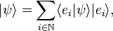
 the inner product on the Hilbert space.
From the commutativity of kets with (complex) scalars now follows that
 ,
,
 ,
,In quantum mechanics, it often occurs that little or no information about the inner product
 of two arbitrary (state) kets is present, while it is still possible to say something about the expansion coefficients
  and
and  of those vectors with respect to a specific (orthonormalized) basis. In this case, it is particularly useful to insert the unit operator into the bracket one time or more.
Notation used by mathematicians
The object physicists are considering when using the "bra-ket" notation is a Hilbert space (a complete inner product space).Let
 be a Hilbert space and
  is a vector in . What physicists would denote as |h⟩ is the vector itself. That is
 .
.
 .
. be the dual space of . This is the space of linear functionals on . The isomorphism
  is defined by
  where for all
  we have
 ,
,
 ,
, and are just different notations for expressing an inner product between two elements in a Hilbert space (or for the first three, in any inner product space). Notational confusion arises when identifying
  and
and  with
with  and
and  respectively. This is because of literal symbolic substitutions. Let
  and let
  . This gives
Moreover, mathematicians usually write the dual entity not at the first place, as the physicists do, but at the second one, and they don't use the *-symbol, but an overline (which the physicists reserve for averages and Dirac conjugation) to denote conjugate-complex numbers, i.e. for scalar products mathematicians usually write