From Wikipedia, the free encyclopedia
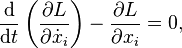
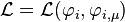
The Lagrangian, L, of a dynamical system is a mathematical function that summarizes the dynamics of the system. For a simple mechanical system, it is the value given by the kinetic energy of the particle minus the potential energy of the particle but it may be generalized to more complex systems. It is used primarily as a key component in the Euler-Lagrange equations to find the path of a particle according to the principle of least action.
The Lagrangian is named after Italian mathematician and astronomer Joseph Louis Lagrange. The concept of a Lagrangian was introduced in a reformulation of classical mechanics introduced by Lagrange known as Lagrangian mechanics in 1788. This reformulation was needed in order to explore mechanics in alternative systems to Cartesian coordinates such as Polar, Cylindrical and Spherical coordinates for which Newtonian mechanics was not suitable.[1]
The Lagrangian has since been used in a method to find the acceleration of a particle in a Newtonian gravitational field and to derive the Einstein field equations. This led to its use in applying electromagnetism to curved spacetime and in describing charged black holes. It also has additional uses in Mathematical formalism to find the functional derivative of an action, and in engineering for the analysis and optimisation of dynamic systems.
Definition
In classical mechanics, the natural form of the Lagrangian is defined as the kinetic energy, T, of the system minus its potential energy, V.[2] In symbols,
 , but solving any equivalent Lagrangians will give the same equations of motion.[3][4]
The Lagrangian formulation
Simple example
The trajectory of a thrown ball is characterized by the sum of the Lagrangian values at each time being a (local) minimum.The Lagrangian L can be calculated at several instants of time t, and a graph of L against t can be drawn. The area under the curve is the action. Any different path between the initial and final positions leads to a larger action than that chosen by nature. Nature chooses the smallest action – this is the Principle of Least Action.
If Nature has defined the mechanics problem of the thrown ball in so elegant a fashion, might She have defined other problems similarly. So it seems now. Indeed, at the present time it appears that we can describe all the fundamental forces in terms of a Lagrangian. The search for Nature's One Equation, which rules all of the universe, has been largely a search for an adequate Lagrangian.Using only the principle of least action and the Lagrangian we can deduce the correct trajectory, by trial and error or the calculus of variations.
—Robert Adair, The Great Design: Particles, Fields, and Creation[5]
Importance
The Lagrangian formulation of mechanics is important not just for its broad applications, but also for its role in advancing deep understanding of physics. Although Lagrange only sought to describe classical mechanics, the action principle that is used to derive the Lagrange equation was later recognized to be applicable to quantum mechanics as well.Physical action and quantum-mechanical phase are related via Planck's constant, and the principle of stationary action can be understood in terms of constructive interference of wave functions.
The same principle, and the Lagrangian formalism, are tied closely to Noether's theorem, which connects physical conserved quantities to continuous symmetries of a physical system.
Lagrangian mechanics and Noether's theorem together yield a natural formalism for first quantization by including commutators between certain terms of the Lagrangian equations of motion for a physical system.
Advantages over other methods
- The formulation is not tied to any one coordinate system – rather, any convenient variables may be used to describe the system; these variables are called "generalized coordinates" qi and may be any quantitative attributes of the system (for example, strength of the magnetic field at a particular location; angle of a pulley; position of a particle in space; or degree of excitation of a particular eigenmode in a complex system) which are functions of the independent variable(s). This trait makes it easy to incorporate constraints into a theory by defining coordinates that only describe states of the system that satisfy the constraints.
- If the Lagrangian is invariant under a symmetry, then the resulting equations of motion are also invariant under that symmetry. This characteristic is very helpful in showing that theories are consistent with either special relativity or general relativity.
Cyclic coordinates and conservation laws
An important property of the Lagrangian is that conservation laws can easily be read off from it. For example, if the Lagrangian does not depend on
  itself, then the generalized momentum (
 ), given by:
 depends on the time derivative
  of that generalized coordinate, since the Lagrangian independence of the coordinate always makes the above partial derivative zero. This is a special case of Noether's theorem. Such coordinates are called "cyclic" or "ignorable".
For example, the conservation of the generalized momentum,


Explanation
The Lagrangian in many classical systems is a function of generalized coordinates qi and their velocities dqi/dt. These coordinates (and velocities) are, in their turn, parametric functions of time. In the classical view, time is an independent variable and qi (and dqi/dt) are dependent variables as is often seen in phase space explanations of systems. This formalism was generalized further to handle field theory. In field theory, the independent variable is replaced by an event in spacetime (x, y, z, t), or more generally still by a point s on a manifold. The dependent variables (q) are replaced by the value of a field at that point in spacetime φ(x,y,z,t) so that the equations of motion are obtained by means of an action principle, written as:
 , is a functional of the dependent variables φi(s) with their derivatives and s itself
![\mathcal{S}\left[\varphi_i\right] = \int{ \mathcal{L} \left(\varphi_i (s), \frac{\partial \varphi_i (s)}{\partial s^\alpha}, s^\alpha\right) \, \mathrm{d}^n s }](http://upload.wikimedia.org/math/a/8/a/a8ada7e2e3a2eafb5bac52b6ae998890.png)
 is used in the case of multiple independent variables (usually four: x, y, z, t).
The equations of motion obtained from this functional derivative are the Euler–Lagrange equations of this action.
For example, in the classical mechanics of particles, the only independent variable is time, t. So the Euler–Lagrange equations are

An example from classical mechanics
In Cartesian coordinates
Suppose we have a three-dimensional space in which a particle of mass m moves under the influence of a conservative force . Since the force is conservative, it corresponds to a potential energy function
  given by
  . The Lagrangian of the particle can be written
Then


In spherical coordinates
Suppose we have a three-dimensional space using spherical coordinates (r, θ, φ) with the Lagrangian


 of the particle.
Despite the use of standard variables such as x, the Lagrangian allows the use of any coordinates, which do not need to be orthogonal. These are "generalized coordinates".
Lagrangian of a test particle
A test particle is a particle whose mass and charge are assumed to be so small that its effect on external system is insignificant. It is often a hypothetical simplified point particle with no properties other than mass and charge. Real particles like electrons and up quarks are more complex and have additional terms in their Lagrangians.Classical test particle with Newtonian gravity
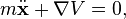
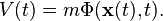
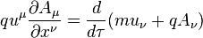
Suppose we are given a particle with mass m kilograms, and position meters in a Newtonian gravitation field with potential Φ in J·kg−1. The particle's world line is parameterized by time t seconds. The particle's kinetic energy is:
 in the integral (equivalent to the Euler–Lagrange differential equation), we get
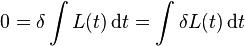


 (1)
(1)

Special relativistic test particle with electromagnetism
In special relativity, the energy (rest energy plus kinetic energy) of a free test particle is
One possible Lagrangian

 The second term in the series is just the classical kinetic energy. Suppose the particle has electrical charge q coulombs and is in an electromagnetic field with scalar potential ϕ volts (a volt is a joule per coulomb) and vector potential
  V·s·m−1. The Lagrangian of a special relativistic test particle in an electromagnetic field is:
 , we get


An alternative Lagrangian for a special relativistic test particle is

The Euler-Lagrange equations

General relativistic test particle
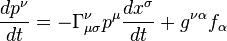
In general relativity, the first term generalizes (includes) both the classical kinetic energy and the interaction with the gravitational field. It becomes:[8][9]

More generally, suppose the Lagrangian is that of a single particle plus an interaction term LI


 .)
.)Rearranging gets the force equation

If we let


Lagrangians and Lagrangian densities in field theory
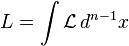
The time integral of the Lagrangian is called the action denoted by S. In field theory, a distinction is occasionally made between the Lagrangian L, of which the action is the time integral:
 , which one integrates over all spacetime to get the action:
![\mathcal{S} [\varphi_i] = \int{\mathcal{L} (\varphi_i (x))\, \mathrm{d}^4x}.](http://upload.wikimedia.org/math/6/d/f/6df53fb1b17f5a37ffb2f84f4d9caae1.png)
- General form of Lagrangian density:
 [10] where
  (see 4-gradient)
 - The relationship between
 and
and  :
:  , where
  is the space-time dimension [10] similar to
  .
. - In field theory, the independent variable t was replaced by an event in spacetime (x, y, z, t) or still more generally by a point s on a manifold.

 (see
(see  :
:  , where
  is the space-time dimension
  . is also frequently simply called the Lagrangian, especially in modern use; it is far more useful in relativistic theories since it is a locally defined, Lorentz scalar field. Both definitions of the Lagrangian can be seen as special cases of the general form, depending on whether the spatial variable
  is incorporated into the index i or the parameters s in φi(s). Quantum field theories in particle physics, such as quantum electrodynamics, are usually described in terms of , and the terms in this form of the Lagrangian translate quickly to the rules used in evaluating Feynman diagrams.
Notice that, in the presence of gravity or when using general curvilinear coordinates, the Lagrangian density
 will include a factor of
  or its equivalent to ensure that it is a scalar density so that the integral will be invariant.
Selected fields
To go with the section on test particles above, here are the equations for the fields in which they move. The equations below pertain to the fields in which the test particles described above move and allow the calculation of those fields. The equations below will not give you the equations of motion of a test particle in the field but will instead give you the potential (field) induced by quantities such as mass or charge density at any point . For example, in the case of Newtonian gravity, the Lagrangian density integrated over spacetime gives you an equation which, if solved, would yield
  . This , when substituted back in equation (1), the Lagrangian equation for the test particle in a Newtonian gravitational field, provides the information needed to calculate the acceleration of the particle.
Newtonian gravity
The Lagrangian (density) is in J·m−3. The interaction term mΦ is replaced by a term involving a continuous mass density ρ in kg·m−3. This is necessary because using a point source for a field would result in mathematical difficulties. The resulting Lagrangian for the classical gravitational field is:


Einstein Gravity
The Lagrange density for general relativity in the presence of matter fields is
 is the curvature scalar, which is the Ricci tensor contracted with the metric tensor, and the Ricci tensor is the Riemann tensor contracted with a Kronecker delta. The integral of
  is known as the Einstein-Hilbert action. The Riemann tensor is the tidal force tensor, and is constructed out of Christoffel symbols and derivatives of Christoffel symbols, which are the gravitational force field. Plugging this Lagrangian into the Euler-Lagrange equation and taking the metric tensor
  as the field, we obtain the Einstein field equations
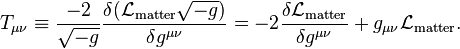
 is the determinant of the metric tensor when regarded as a matrix.
  is the Cosmological constant. Generally, in general relativity, the integration measure of the action of Lagrange density is
  . This makes the integral coordinate independent, as the root of the metric determinant is equivalent to the Jacobian determinant. The minus sign is a consequence of the metric signature (the determinant by itself is negative).[11]
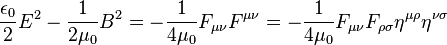
Electromagnetism in special relativity
The interaction terms
 in A·m−2. The resulting Lagrangian for the electromagnetic field is:

Varying instead with respect to
, we get
Using tensor notation, we can write all this more compactly. The term
 is actually the inner product of two four-vectors. We package the charge density into the current 4-vector and the potential into the potential 4-vector. These two new vectors are
 . We define this tensor as
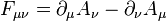


Electromagnetism in general relativity
The Lagrange density of electromagnetism in general relativity also contains the Einstein-Hilbert action from above. The pure electromagnetic Lagrangian is precisely a matter Lagrangian . The Lagrangian is
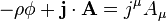
 . We can generate the Einstein Field Equations in the presence of an EM field using this lagrangian. The energy-momentum tensor is


 is the covariant derivative. For free space, we can set the current tensor equal to zero,
  . Solving both Einstein and Maxwell's equations around a spherically symmetric mass distribution in free space leads to the Reissner-Nordstrom charged black hole, with the defining line element (written in natural units and with charge Q):
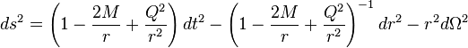
Electromagnetism using differential forms
Using differential forms, the electromagnetic action S in vacuum on a (pseudo-) Riemannian manifold can be written (using natural units, c = ε0 = 1) as
![\mathcal S[\mathbf{A}] = \int_{\mathcal{M}} \left(-\frac{1}{2}\,\mathbf{F} \wedge \star\mathbf{F} + \mathbf{A} \wedge\star \mathbf{J}\right) .](http://upload.wikimedia.org/math/a/e/d/aed8024178fc3125ef96615977ec262f.png)


Dirac Lagrangian
The Lagrangian density for a Dirac field is:[15]
 is its Dirac adjoint (creation operator), and
  is Feynman slash notation for
  .
.Quantum electrodynamic Lagrangian
The Lagrangian density for QED is: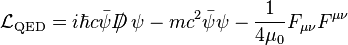
 is the electromagnetic tensor, D is the gauge covariant derivative, and
  is Feynman notation for
  .
.Quantum chromodynamic Lagrangian
The Lagrangian density for quantum chromodynamics is:[16][17][18]
 is the gluon field strength tensor.
Mathematical formalism
Suppose we have an n-dimensional manifold, M, and a target manifold, T. Let be the configuration space of smooth functions from M to T.
Examples
- In classical mechanics, in the Hamiltonian formalism, M is the one-dimensional manifold
 , representing time and the target space is the cotangent bundle of space of generalized positions.
 - In field theory, M is the spacetime manifold and the target space is the set of values the fields can take at any given point. For example, if there are m real-valued scalar fields, ϕ1, ..., ϕm, then the target manifold is
 . If the field is a real vector field, then the target manifold is isomorphic to
  . There is actually a much more elegant way using tangent bundles over M, but we will just stick to this version.
 . If the field is a real
  . There is actually a much more elegant way using
 Mathematical development
Consider a functional, ,
,
 ,
, (the set of all real numbers), not
  (the set of all complex numbers).
In order for the action to be local, we need additional restrictions on the action. If
 , we assume
 ![\scriptstyle\mathcal{S}[\varphi]](http://upload.wikimedia.org/math/4/f/e/4feacf4d2075e1f71f567da32bd2f265.png) is the integral over M of a function of
is the integral over M of a function of  , its derivatives and the position called the Lagrangian,
  . In other words,
![\forall\varphi\in\mathcal{C}, \ \ \mathcal{S}[\varphi]\equiv\int_M \mathrm{d}^nx \mathcal{L} \big( \varphi(x),\partial\varphi(x),\partial\partial\varphi(x), ...,x \big).](http://upload.wikimedia.org/math/a/8/d/a8dfb1ebe45498e228103ee0753c7fe4.png)
Given boundary conditions, basically a specification of the value of
at the boundary if M is compact or some limit on as x → ∞ (this will help in doing integration by parts), the subspace of consisting of functions, , such that all functional derivatives of S at are zero and satisfies the given boundary conditions is the subspace of on shell solutions.The solution is given by the Euler–Lagrange equations (thanks to the boundary conditions),
 .
.Uses in Engineering
Circa 1963[when?] Lagrangians were a general part of the engineering curriculum, but a quarter of a century later, even with the ascendency of dynamical systems, they were dropped as requirements for some engineering programs, and are generally considered to be the domain of theoretical dynamics. Circa 2003[when?] this changed dramatically, and Lagrangians are not only a required part of many ME and EE graduate-level curricula, but also find applications in finance, economics, and biology, mainly as the basis of the formulation of various path integral schemes to facilitate the solution of parabolic partial differential equations via random walks.Circa 2013,[when?] Lagrangians find their way into hundreds of direct engineering solutions, including robotics, turbulent flow analysis (Lagrangian and Eulerian specification of the flow field), signal processing, microscopic component contact and nanotechnology (superlinear convergent augmented Lagrangians), gyroscopic forcing and dissipation, semi-infinite supercomputing (which also involve Lagrange multipliers in the subfield of semi-infinite programming), chemical engineering (specific heat linear Lagrangian interpolation in reaction planning), civil engineering (dynamic analysis of traffic flows), optics engineering and design (Lagrangian and Hamiltonian optics) aerospace (Lagrangian interpolation), force stepping integrators, and even airbag deployment (coupled Eulerian-Lagrangians as well as SELM—the stochastic Eulerian Lagrangian method).[19]