From Wikipedia, the free encyclopedia

Graph of a function of total emitted energy of a black body  proportional to its thermodynamic temperature
  . In blue is a total energy according to the Wien approximation,
 proportional to its thermodynamic temperature
  . In blue is a total energy according to the Wien approximation,
The Stefan–Boltzmann law, also known as Stefan's law, describes the power radiated from a black body in terms of its temperature. Specifically, the Stefan–Boltzmann law states that the total energy radiated per unit surface area of a black body across all wavelengths per unit time (also known as the black-body radiant exitance or emissive power),
, is directly proportional to the fourth power of the black body's thermodynamic temperature T:
 :
: has dimensions of energy flux (energy per time per area), and the SI units of measure are joules per second per square metre, or equivalently, watts per square metre. The SI unit for absolute temperature T is the kelvin.
  is the emissivity of the grey body; if it is a perfect blackbody,
  . In the still more general (and realistic) case, the emissivity depends on the wavelength,
  .
.To find the total power radiated from an object, multiply by its surface area,
 :
:
History
The law was deduced by Jožef Stefan (1835–1893) in 1879 on the basis of experimental measurements made by John Tyndall and was derived from theoretical considerations, using thermodynamics, by Ludwig Boltzmann (1844–1906) in 1884. Boltzmann considered a certain ideal heat engine with light as a working matter instead of gas. The law is highly accurate only for ideal black objects, the perfect radiators, called black bodies; it works as a good approximation for most "grey" bodies. Stefan published this law in the article Über die Beziehung zwischen der Wärmestrahlung und der Temperatur (On the relationship between thermal radiation and temperature) in the Bulletins from the sessions of the Vienna Academy of Sciences.Examples
Temperature of the Sun
With his law Stefan also determined the temperature of the Sun's surface. He learned from the data of Charles Soret (1854–1904) that the energy flux density from the Sun is 29 times greater than the energy flux density of a certain warmed metal lamella (a thin plate). A round lamella was placed at such a distance from the measuring device that it would be seen at the same angle as the Sun. Soret estimated the temperature of the lamella to be approximately 1900 °C to 2000 °C. Stefan surmised that ⅓ of the energy flux from the Sun is absorbed by the Earth's atmosphere, so he took for the correct Sun's energy flux a value 3/2 times greater than Soret's value, namely 29 × 3/2 = 43.5.Precise measurements of atmospheric absorption were not made until 1888 and 1904. The temperature Stefan obtained was a median value of previous ones, 1950 °C and the absolute thermodynamic one 2200 K. As 2.574 = 43.5, it follows from the law that the temperature of the Sun is 2.57 times greater than the temperature of the lamella, so Stefan got a value of 5430 °C or 5700 K (the modern value is 5778 K[3]). This was the first sensible value for the temperature of the Sun. Before this, values ranging from as low as 1800 °C to as high as 13,000,000 °C were claimed. The lower value of 1800 °C was determined by Claude Servais Mathias Pouillet (1790–1868) in 1838 using the Dulong-Petit law. Pouillet also took just half the value of the Sun's correct energy flux.
Temperature of stars
The temperature of stars other than the Sun can be approximated using a similar means by treating the emitted energy as a black body radiation.[4] So:
 , is the solar radius, and so forth.
With the Stefan–Boltzmann law, astronomers can easily infer the radii of stars. The law is also met in the thermodynamics of black holes in so-called Hawking radiation.
Temperature of the Earth
Similarly we can calculate the effective temperature of the Earth TE by equating the energy received from the Sun and the energy radiated by the Earth, under the black-body approximation. The amount of power, ES, emitted by the Sun is given by:

 . The amount of solar power absorbed by the Earth is thus given by:

The Earth has an albedo of 0.3, meaning that 30% of the solar radiation that hits the planet gets scattered back into space without absorption. The effect of albedo on temperature can be approximated by assuming that the energy absorbed is multiplied by 0.7, but that the planet still radiates as a black body (the latter by definition of effective temperature, which is what we are calculating). This approximation reduces the temperature by a factor of 0.71/4, giving 255 K (−18 °C).[5][6]
However, long-wave radiation from the surface of the earth is partially absorbed and re-radiated back down by greenhouse gases, namely water vapor, carbon dioxide and methane.[7][8] Since the emissivity with greenhouse effect (weighted more in the longer wavelengths where the Earth radiates) is reduced more than the absorptivity (weighted more in the shorter wavelengths of the Sun's radiation) is reduced, the equilibrium temperature is higher than the simple black-body calculation estimates. As a result, the Earth's actual average surface temperature is about 288 K (15 °C), which is higher than the 255 K effective temperature, and even higher than the 279 K temperature that a black body would have.
Origination
Thermodynamic derivation of the energy density
The fact that the energy density of the box containing radiation is proportional to can be derived using thermodynamics. It follows from the Maxwell stress tensor of classical electrodynamics that the radiation pressure
  is related to the internal energy density
  :
: .
.From the fundamental thermodynamic relation
 ,
,we obtain the following expression, after dividing by
 and fixing
  :
: .
.The last equality comes from the following Maxwell relation:
 .
.From the definition of energy density it follows that

where the energy density of radiation only depends on the temperature, therefore
 .
.Now, the equality
 ,
,after substitution of
 and for the corresponding expressions, can be written as
 .
.Since the partial derivative
 can be expressed as a relationship between only and (if one isolates it on one side of the equality), the partial derivative can be replaced by the ordinary derivative. After separating the differentials the equality becomes
 ,
,which leads immediately to
 , with as some constant of integration.
Stefan–Boltzmann's law in n-dimensional space
It can be shown that the radiation pressure in -dimensional space is given by[10]
So in
-dimensional space,


 -dimensional space, albeit with a different value for the Stefan-Boltzmann constant at each dimension. In general the constant is
where
 [
[ is Riemann's zeta function and
  is a certain function of , with
  .
.Derivation from Planck's law
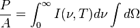
The law can be derived by considering a small flat black body surface radiating out into a half-sphere. This derivation uses spherical coordinates, with φ as the zenith angle and θ as the azimuthal angle; and the small flat blackbody surface lies on the xy-plane, where φ = π/2.The intensity of the light emitted from the blackbody surface is given by Planck's law :
-
- where
 is the amount of power per unit surface area per unit solid angle per unit frequency emitted at a frequency
  by a black body at temperature T.
 is Planck's constant
 is the speed of light, and
 is Boltzmann's constant.

 is the amount of
  by a black body at temperature T.
 is
is  is the
  is
is  is the power radiated by a surface of area A through a solid angle dΩ in the frequency range between ν and ν + dν.
The Stefan–Boltzmann law gives the power emitted per unit area of the emitting body,
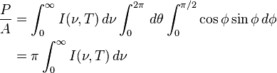


 , giving the result that, for a perfect blackbody surface:
Appendix
In one of the above derivations, the following integral appeared:
 is the polylogarithm function and
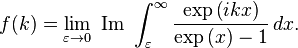
  is the Riemann zeta function. If the polylogarithm function and the Riemann zeta function are not available for calculation, there are a number of ways to do this integration; a simple one is given in the appendix of the Planck's law article. This appendix does the integral by contour integration. Consider the function:
 , we see that
  is minus 6 times the coefficient of
  of the series expansion of
  . So, if we can find a closed form for f(k), its Taylor expansion will give J.
In turn, sin(x) is the imaginary part of eix, so we can restate this as:

 is the contour from to
  , then to
  , then to
  , then we go to the point
  , avoiding the pole at
  by taking a clockwise quarter circle with radius and center . From there we go to
  , and finally we return to , avoiding the pole at zero by taking a clockwise quarter circle with radius and center zero.
Because there are no poles in the integration contour we have:

 . In this limit the contribution from the segment from to tends to zero. Taking together the integrations over the segments from to and from to and using the fact that the integrations over clockwise quarter circles withradius about simple poles are given up to order by minus
  times the residues at the poles we find:
![\left[1-\exp\left(-2\pi k\right) \right]\int_\varepsilon^\infty \frac{\exp\left(ikx\right)}{\exp\left(x\right)-1} \, dx = i \int_\varepsilon^{2\pi-\varepsilon} \frac{\exp\left(-ky\right)}{\exp\left(iy\right)-1} \, dy + i\frac{\pi}{2}\left[1 + \exp \left(-2\pi k\right)\right] + \mathcal{O} \left(\varepsilon\right) \qquad \text{ (1)}](http://upload.wikimedia.org/math/d/d/2/dd2de29c20f3714f026b0eab036fd12e.png)
The left hand side is the sum of the integral from
to and from to  . We can rewrite the integrand of the integral on the r.h.s. as follows:
 we find:
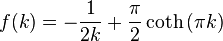

 is given by:
 of the series expansion of is
  . This then implies that
  and the result


