Solar irradiance

From Wikipedia, the free encyclopedia

Solar irradiance (also Insolation, from Latin insolare, to expose to the sun)^[1][2] is the power per unit area produced by the Sun in the form of electromagnetic radiation. Irradiance may be measured in space or at the Earth's surface after atmospheric absorption and scattering. Total solar irradiance (TSI), is a measure of the solar radiative power per unit area normal to the rays, incident on the Earth's upper atmosphere. The solar constant is a conventional measure of mean TSI at a distance of one Astronomical Unit (AU). Irradiance is a function of distance from the Sun, the solar cycle, and cross-cycle changes.^[3] Irradiance on Earth is most intense at points directly facing (normal to) the Sun.

Annual mean insolation at the top of Earth's atmosphere (TOA) and at the planet's surface

Units

The unit recommended by the World Meteorological Organization is the megajoule per square metre (MJ/m²) or joule per square millimetre (J/mm²).^[4]

An alternate unit of measure is the Langley (1 thermochemical calorie per square centimeter or 41,840 J/m²) or irradiance per unit time.

The solar energy business uses watt-hour per square metre (Wh/m²). Divided by the recording time, this measure becomes insolation, another unit of irradiance.

Insolation can be measured in space, at the edge of the atmosphere or at a terrestrial object.
Insolation can also be expressed in Suns, where one Sun equals 1000 W/m² at the point of arrival, with kWh/m²/day expressed as hours/day.^[5]

Absorption and reflection[edit source | edit]

Reaching an object, part of the irradiance is absorbed and the remainder reflected. Usually the absorbed radiation is converted to thermal energy, increasing the object's temperature. Manmade or natural systems, however, can convert part of the absorbed radiation into another form such as electricity or chemical bonds, as in the case of photovoltaic cells or plants. The proportion of reflected radiation is the object's reflectivity or albedo.

Projection effect

One sunbeam one mile wide shines on the ground at a 90° angle, and another at a 30° angle. The oblique sunbeam distributes its light energy over twice as much area.

Insolation onto a surface is largest when the surface directly faces (is normal to) the sun. As the angle between the surface and the Sun moves from normal, the insolation is reduced in proportion to the angle's Cosine; see Effect of sun angle on climate.

In the figure, the angle shown is between the ground and the sunbeam rather than between the vertical direction and the sunbeam; hence the sine rather than the cosine is appropriate. A sunbeam one mile (1.6 km) wide arrives from directly overhead, and another at a 30° angle to the horizontal. The Sine of a 30° angle is 1/2, whereas the sine of a 90° angle is 1. Therefore, the angled sunbeam spreads the light over twice the area. Consequently, half as much light falls on each square mile.

This 'projection effect' is the main reason why Earth's polar regions are much colder than equatorial regions. On an annual average the poles receive less insolation than does the equator, because the poles are always angled more away from the sun than the tropics. At a lower angle the light must travel through more atmosphere. This attenuates it (by absorption and scattering) further reducing insolation.

Categories

Solar potential – global horizontal irradiation

Direct insolation is measured at a given location with a surface element perpendicular to the Sun. It excludes diffuse insolation (radiation that is scattered or reflected by atmospheric components). Direct insolation is equal to the Solar constant minus the atmospheric losses due to absorption and scattering. While the solar constant varies, losses depend on time of day (length of light's path through the atmosphere depending on the Solar elevation angle), Cloud cover, Moisture content and other contents. Insolation affects plant metabolism and animal behavior.^[6]

Diffuse insolation is the contribution of light scattered by the atmosphere to total insolation.

Earth

Average annual solar radiation arriving at the top of the Earth's atmosphere is roughly 1366 W/m².^[7][8] The radiation is distributed across the Electromagnetic spectrum, although most is Visible light. The Sun's rays are attenuated as they pass through the Atmosphere, leaving maximum normal surface irradiance at approximately 1000 W /m² at Sealevel on a clear day.^{[clarification needed]}

A Pyranometer, a component of a temporary remote meteorological station, measures insolation on Skagit Bay, Washington.

The actual figure varies with the Sun's angle and atmospheric circumstances. Ignoring clouds, the daily average irradiance for the Earth is approximately 6 kWh/m² = 21.6 MJ/m². The output of, for example, a photovoltaic panel, partly depends on the angle of the sun relative to the panel. One Sun is a unit of power flux, not a standard value for actual insolation. Sometimes this unit is referred to as a Sol, not to be confused with a sol, meaning one solar day.^[9]

Solar potential maps

• 

  North America
• 

  South America
• 

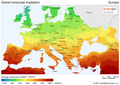  Europe
• 

  Africa and Middle East
• 

  South and South-East Asia
• 

  Australia

Top of the atmosphere

Spherical triangle for application of the spherical law of cosines for the calculation the solar zenith angle Θ for observer at latitude φ and longitude λ from knowledge of the hour angle h and solar declination δ. (δ is latitude of subsolar point, and h is relative longitude of subsolar point).

, the theoretical daily-average insolation at the top of the atmosphere, where θ is the polar angle of the Earth's orbit, and θ = 0 at the vernal equinox, and θ = 90° at the summer solstice; φ is the latitude of the Earth. The calculation assumed conditions appropriate for 2000 A.D.: a solar constant of S₀ = 1367 W m⁻², obliquity of ε = 23.4398°, longitude of perihelion of ϖ = 282.895°, eccentricity e = 0.016704. Contour labels (green) are in units of W m⁻².

The distribution of solar radiation at the top of the atmosphere is determined by Earth's sphericity and orbital parameters. This applies to any unidirectional beam incident to a rotating sphere. Insolation is essential for numerical weather prediction and understanding seasons and climate change. Application to ice ages is known as Milankovitch cycles.

Distribution is based on a fundamental identity from Spherical trigonometry, the spherical law of cosines:

 

where a, b and c are arc lengths, in radians, of the sides of a spherical triangle. C is the angle in the vertex opposite the side which has arc length c. Applied to the calculation of Solar zenith angle Θ, the following applies to the Spherical law of cosines:

The separation of Earth from the sun can be denoted R_E and the mean distance can be denoted R₀, approximately 1 AU. The solar constant is denoted S₀. The solar flux density (insolation) onto a plane tangent to the sphere of the Earth, but above the bulk of the atmosphere (elevation 100 km or greater) is:

and

The average of Q over a day is the average of Q over one rotation, or the hour angle progressing from h = π to h = −π:

Let h₀ be the hour angle when Q becomes positive. This could occur at sunrise when , or for h₀ as a solution of

or

If tan(φ)tan(δ) > 1, then the sun does not set and the sun is already risen at h = π, so h_o = π. If tan(φ)tan(δ) < −1, the sun does not rise and .

is nearly constant over the course of a day, and can be taken outside the integral

Let θ be the conventional polar angle describing a planetary orbit. Let θ = 0 at the vernal equinox. The declination δ as a function of orbital position is

where ε is the obliquity. The conventional longitude of perihelion ϖ is defined relative to the vernal equinox, so for the elliptical orbit:

or

With knowledge of ϖ, ε and e from astrodynamical calculations ^[10] and S_o from a consensus of observations or theory, can be calculated for any latitude φ and θ. Because of the elliptical orbit, and as a consequence of Kepler's second law, θ does not progress uniformly with time. Nevertheless, θ = 0° is exactly the time of the vernal equinox, θ = 90° is exactly the time of the summer solstice, θ = 180° is exactly the time of the autumnal equinox and θ = 270° is exactly the time of the winter solstice.

Variation

Total irradiance

Total solar irradiance (TSI)^[11] changes slowly on decadal and longer timescales. The variation during solar cycle 21 was about 0.1% (peak-to-peak).^[12] In contrast to older reconstructions,^[13] most recent TSI reconstructions point to an increase of only about 0.05% to 0.1% between the Maunder Minimum and the present.^[14][15][16]

Ultraviolet irradiance

Ultraviolet irradiance (EUV) varies by approximately 1.5 percent from solar maxima to minima, for 200 to 300 nm wavelengths.^[17] However, a proxy study estimated that UV has increased by 3.0% since the Maunder Minimum.^[18]

Milankovitch cycles

Some variations in insolation are not due to solar changes but rather due to the Earth moving between its perigee and apogee, or changes in the latitudinal distribution of radiation. These orbital changes or Milankovitch cycles have caused radiance variations of as much as 25% (locally; global average changes are much smaller) over long periods. The most recent significant event was an axial tilt of 24° during boreal summer near the Holocene climatic optimum.

Obtaining a time series for a for a particular time of year, and particular latitude, is a useful application in the theory of Milankovitch cycles. For example, at the summer solstice, the declination δ is equal to the obliquity ε. The distance from the sun is

For this summer solstice calculation, the role of the elliptical orbit is entirely contained within the important product , the precession index, whose variation dominates the variations in insolation at 65° N when eccentricity is large. For the next 100,000 years, with variations in eccentricity being relatively small, variations in obliquity dominate.

Measurement

The space-based TSI record comprises measurements from more than ten radiometers spanning three solar cycles.

Technique

All modern TSI satellite instruments employ active cavity electrical substitution radiometry. This technique applies measured electrical heating to maintain an absorptive blackened cavity in thermal equilibrium while incident sunlight passes through a precision aperture of calibrated area. The aperture is modulated via a shutter. Accuracy uncertainties of <0.01% are required to detect long term solar irradiance variations, because expected changes are in the range 0.05 to 0.15 W m−2 per century.^[19]

Intertemporal calibration

In orbit, radiometric calibrations drift for reasons including solar degradation of the cavity, electronic degradation of the heater, surface degradation of the precision aperture and varying surface emissions and temperatures that alter thermal backgrounds. These calibrations require compensation to preserve consistent measurements.^[19]

For various reasons, the sources do not always agree. The Solar Radiation and Climate Experiment/Total Irradiance Measurement (SORCE/TIM) TSI values are lower than prior measurements by the Earth Radiometer Budget Experiment (ERBE) on the Earth Radiation Budget Satellite (ERBS), VIRGO on the Solar Heliospheric Observatory (SoHO) and the ACRIM instruments on the Solar Maximum Mission (SMM), Upper Atmosphere Research Satellite (UARS) and ACRIMSat. Pre-launch ground calibrations relied on component rather than system level measurements, since irradiance standards lacked absolute accuracies.^[19]

Measurement stability involves exposing different radiometer cavities to different accumulations of solar radiation to quantify exposure-dependent degradation effects. These effects are then compensated for in final data. Observation overlaps permits corrections for both absolute offsets and validation of instrumental drifts.^[19]

Uncertainties of individual observations exceed irradiance variability (∼0.1%). Thus, instrument stability and measurement continuity are relied upon to compute real variations.

Long-term radiometer drifts can be mistaken for irradiance variations that can be misinterpreted as affecting climate. Examples include the issue of the irradiance increase between cycle minima in 1986 and 1996, evident only in the ACRIM composite (and not the model) and the low irradiance levels in the PMOD composite during the 2008 minimum.

Despite the fact that ACRIM I, ACRIM II, ACRIM III, VIRGO and TIM all track degradation with redundant cavities, notable and unexplained differences remain in irradiance and the modeled influences of sunspots and faculae.

Persistent inconsistencies

Disagreement among overlapping observations indicates unresolved drifts that suggest the TSI record is not sufficiently stable to discern solar changes on decadal time scales. Only the ACRIM composite shows irradiance increasing by ∼1 W m−2 between 1986 and 1996; this change is also absent in the model.^[19]

Recommendations to resolve the instrument discrepancies include validating optical measurement accuracy by comparing ground-based instruments to laboratory references, such as those at National Institute of Science and Technology (NIST); NIST validation of aperture area calibrations uses spares from each instrument; and applying diffraction corrections from the view-limiting aperture.^[19]

For ACRIM, NIST determined that diffraction from the view-limiting aperture contributes a 0.13% signal not accounted for in the three ACRIM instruments. This correction lowers the reported ACRIM values, bringing ACRIM closer to TIM. In ACRIM and all other instruments, the aperture is deep inside the instrument, with a larger view-limiting aperture at the front. Depending on edge imperfections this can directly scatter light into the cavity. This design admits two to three times the amount of light intended to be measured; if not completely absorbed or scattered, this additional light produces erroneously high signals. In contrast, TIM's design places the precision aperture at the front so that only desired light enters.^[19]

Variations from other sources likely include an annual cycle that is nearly in phase with the Sun-Earth distance in ACRIM III data and 90-day spikes in the VIRGO data coincident with SoHO spacecraft maneuvers that were most apparent during the 2008 solar minimum.

TSI Radiometer Facility

TIM's high absolute accuracy creates new opportunities for measuring climate variables. TSI Radiometer Facility (TRF) is a cryogenic radiometer that operates in a vacuum with controlled light sources. L-1 Standards and Technology (LASP) designed and built the system, completed in 2008. It was calibrated for optical power against the NIST Primary Optical Watt Radiometer, a cryogenic radiometer that maintains the NIST radiant power scale to an uncertainty of 0.02% (1σ). As of 2011 TRF was the only facility that approached the desired <0.01% uncertainty for pre-launch validation of solar radiometers measuring irradiance (rather than merely optical power) at solar power levels and under vacuum conditions.^[19]

TRF encloses both the reference radiometer and the instrument under test in a common vacuum system that contains a stationary, spatially uniform illuminating beam. A precision aperture with area calibrated to 0.0031% (1σ) determines the beam's measured portion. The test instrument's precision aperture is positioned in the same location, without optically altering the beam, for direct comparison to the reference. Variable beam power provides linearity diagnostics, and variable beam diameter diagnoses scattering from different instrument components.^[19]

The Glory/TIM and PICARD/PREMOS flight instrument absolute scales are now traceable to the TRF in both optical power and irradiance. The resulting high accuracy reduces the consequences of any future gap in the solar irradiance record.^[19]

Difference Relative to TRF^[19]

Instrument	Irradiance: View-Limiting Aperture Overfilled	Irradiance: Precision Aperture Overfilled	Difference Attributable To Scatter Error	Measured Optical Power Error	Residual Irradiance Agreement	Uncertainty
SORCE/TIM ground	NA	−0.037%	NA	−0.037%	0.000%	0.032%
Glory/TIM flight	NA	−0.012%	NA	−0.029%	0.017%	0.020%
PREMOS-1 ground	−0.005%	−0.104%	0.098%	−0.049%	−0.104%	∼0.038%
PREMOS-3 flight	0.642%	0.605%	0.037%	0.631%	−0.026%	∼0.027%
VIRGO-2 ground	0.897%	0.743%	0.154%	0.730%	0.013%	∼0.025%

2011 reassessment

The most probable value of TSI representative of solar minimum is 1360.8 ± 0.5 W m−2, lower than the earlier accepted value of 1365.4 ± 1.3 W m−2, established in the 1990s. The new value came from SORCE/TIM and radiometric laboratory tests. Scattered light is a primary cause of the higher irradiance values measured by earlier satellites in which the precision aperture is located behind a larger, view-limiting aperture. The TIM uses a view-limiting aperture that is smaller than precision aperture that precludes this spurious signal. The new estimate is from better measurement rather than a change in solar output.^[19]

A regression model-based split of the relative proportion of sunspot and facular influences from SORCE/TIM data accounts for 92% of observed variance and tracks the observed trends to within TIM's stability band. This agreement provides further evidence that TSI variations are primarily due to solar surface magnetic activity.^[19]

Instrument inaccuracies add a significant uncertainty in determining Earth's energy balance. The energy imbalance has been variously measured (during a deep solar minimum of 2005–2010) to be +0.58 ± 0.15 W/m²),^[20] +0.60 ± 0.17 W/m²^[21] and +0.85 W m−2. Estimates from space-based measurements range from +3 to 7 W m−2. SORCE/TIM's lower TSI value reduces this discrepancy by 1 W m−2. This difference between the new lower TIM value and earlier TSI measurements corresponds to a climate forcing of −0.8 W m−2, which is comparable to the energy imbalance.^[19]

2014 reassessment

In 2014 a new ACRIM composite was developed using the updated ACRIM3 record. It added corrections for scattering and diffraction revealed during recent testing at TRF and two algorithm updates. The algorithm updates more accurately account for instrument thermal behavior and parsing of shutter cycle data. These corrected a component of the quasi-annual signal and increased the signal to noise ratio, respectively. The net effect of these corrections decreased the average ACRIM3 TSI value without affecting the trending in the ACRIM Composite TSI.^[22]

Differences between ACRIM and PMOD TSI composites are evident, but the most significant is the solar minimum-to-minimum trends during solar cycles 21-23. ACRIM established an increase of +0.037%/decade from 1980 to 2000 and a decrease thereafter. PMOD instead presents a steady decrease since 1978. Significant differences can also be seen during the peak of solar cycles 21 and 22. These arise from the fact that ACRIM uses the original TSI results published by the satellite experiment teams while PMOD significantly modifies some results to conform them to specific TSI proxy models. The implications of increasing TSI during the global warming of the last two decades of the 20th century are that solar forcing may be a significantly larger factor in climate change than represented in the CMIP5 general circulation climate models.^[22]

Applications

Buildings

In construction, insolation is an important consideration when designing a building for a particular site.^[23]

Insolation variation by month; 1984–1993 averages for January (top) and April (bottom)

The projection effect can be used to design buildings that are cool in summer and warm in winter, by providing vertical windows on the equator-facing side of the building (the south face in the northern hemisphere, or the north face in the southern hemisphere): this maximizes insolation in the winter months when the Sun is low in the sky and minimizes it in the summer when the Sun is high. (The Sun's north/south path through the sky spans 47 degrees through the year).

Solar power

Insolation figures are used as an input to worksheets to size solar power systems.^[24] Because (except for asphalt solar collectors)^[25] panels are almost always mounted at an angle^[26] towards the sun, insolation must be adjusted to prevent estimates that are inaccurately low for winter and inaccurately high for summer.^[27] In many countries the figures can be obtained from an insolation map or from insolation tables that reflect data over the prior 30–50 years. Photovoltaic panels are rated under standard conditions to determine the Wp rating (watts peak),^[28] which can then be used with insolation to determine the expected output, adjusted by factors such as tilt, tracking and shading (which can be included to create the installed Wp rating).^[29] Insolation values range from 800 to 950 kWh/(kWp·y) in Norway to up to 2,900 in Australia.

Climate research

Irradiance plays a part in climate modeling and weather forecasting. A non-zero average global net radiation at the top of the atmosphere is indicative of Earth's thermal disequilibrium as imposed by climate forcing.

The impact of the lower 2014 TSI value on climate models is unknown. A few tenths of a percent change in the absolute TSI level is typically considered to be of minimal consequence for climate simulations. The new measurements require climate model parameter adjustments.

Experiments with GISS Model 3 investigated the sensitivity of model performance to the TSI absolute value during present and pre-industrial epochs, and describe, for example, how the irradiance reduction is partitioned between the atmosphere and surface and the effects on outgoing radiation.^[19]

Assessing the impact of long-term irradiance changes on climate requires greater instrument stability^[19] combined with reliable global surface temperature observations to quantify climate response processes to radiative forcing on decadal time scales. The observed 0.1% irradiance increase imparts 0.22 W m−2 climate forcing, which suggests a transient climate response of 0.6 °C per W m−2. This response is larger by a factor of 2 or more than in the IPCC-assessed 2008 models, possibly appearing in the models' heat uptake by the ocean.^[19]

Space travel

Insolation is the primary variable affecting equilibrium temperature in spacecraft design and planetology.

Solar activity and irradiance measurement is a concern for space travel. For example, the American space agency, NASA, launched its Solar Radiation and Climate Experiment (SORCE) satellite with Solar Irradiance Monitors.^[3]

Civil engineering

In civil engineering and hydrology, numerical models of snowmelt runoff use observations of insolation. This permits estimation of the rate at which water is released from a melting snowpack. Field measurement is accomplished using a pyranometer.

Conversion factor (multiply top row by factor to obtain side column)
	W/m2	kW·h/(m2·day)	sun hours/day	kWh/(m2·y)	kWh/(kWp·y)
W/m2	1	41.66666	41.66666	0.1140796	0.1521061
kW·h/(m2·day)	0.024	1	1	0.0027379	0.0036505
sun hours/day	0.024	1	1	0.0027379	0.0036505
kWh/(m2·y)	8.765813	365.2422	365.2422	1	1.333333
kWh/(kWp·y)	6.574360	273.9316	273.9316	0.75	1

Kinetic theory of gases

From Wikipedia, the free encyclopedia

The temperature of an ideal monatomic gas is proportional to the average kinetic energy of its atoms. The size of helium atoms relative to their spacing is shown to scale under 1950 atmospheres of pressure. The atoms have a certain, average speed, slowed down here two trillion fold from room temperature.

Kinetic theory defines temperature in its own way, not identical with the thermodynamic definition.^[1]

Under a microscope, the molecules making up a liquid are too small to be visible, but the jittering motion of pollen grains or dust particles can be seen. Known as Brownian motion, it results directly from collisions between the grains or particles and liquid molecules. As analyzed by Albert Einstein in 1905, this experimental evidence for kinetic theory is generally seen as having confirmed the concrete material existence of atoms and molecules.

Assumptions

The theory for ideal gases makes the following assumptions:

• The gas consists of very small particles known as molecules. This smallness of their size is such that the total volume of the individual gas molecules added up is negligible compared to the volume of the smallest open ball containing all the molecules. This is equivalent to stating that the average distance separating the gas particles is large compared to their size.
• These particles have the same mass.
• The number of molecules is so large that statistical treatment can be applied.
• These molecules are in constant, random, and rapid motion.
• The rapidly moving particles constantly collide among themselves and with the walls of the container. All these collisions are perfectly elastic. This means, the molecules are considered to be perfectly spherical in shape, and elastic in nature.
• Except during collisions, the interactions among molecules are negligible. (That is, they exert no forces on one another.)

This implies:

1. Relativistic effects are negligible.

2. Quantum-mechanical effects are negligible. This means that the inter-particle distance is much larger than the thermal de Broglie wavelength and the molecules are treated as classical objects.

3. Because of the above two, their dynamics can be treated classically. This means, the equations of motion of the molecules are time-reversible.

• The average kinetic energy of the gas particles depends only on the absolute temperature of the system. The kinetic theory has its own definition of temperature, not identical with the thermodynamic definition.
• The time during collision of molecule with the container's wall is negligible as compared to the time between successive collisions.
• Because they have mass, the gas molecules will be affected by gravity.

More modern developments relax these assumptions and are based on the Boltzmann equation. These can accurately describe the properties of dense gases, because they include the volume of the molecules. The necessary assumptions are the absence of quantum effects, molecular chaos and small gradients in bulk properties. Expansions to higher orders in the density are known as virial expansions.

An important book on kinetic theory is that by Chapman and Cowling.^[1] An important approach to the subject is called Chapman–Enskog theory.^[2] There have been many modern developments and there is an alternative approach developed by Grad based on moment expansions.^[3] In the other limit, for extremely rarefied gases, the gradients in bulk properties are not small compared to the mean free paths. This is known as the Knudsen regime and expansions can be performed in the Knudsen number.

Properties

Pressure and kinetic energy

Pressure is explained by kinetic theory as arising from the force exerted by molecules or atoms impacting on the walls of a container. Consider a gas of N molecules, each of mass m, enclosed in a cuboidal container of volume V=L³. When a gas molecule collides with the wall of the container perpendicular to the x coordinate axis and bounces off in the opposite direction with the same speed (an elastic collision), then the momentum lost by the particle and gained by the wall is:

where v_x is the x-component of the initial velocity of the particle.

The particle impacts one specific side wall once every

(where L is the distance between opposite walls).

The force due to this particle is:

The total force on the wall is

where the bar denotes an average over the N particles. Since the assumption is that the particles move in random directions, we will have to conclude that if we divide the velocity vectors of all particles in three mutually perpendicular directions, the average value along each direction must be equal (though their proportions are arbitrary for individual particles). That is,

.

We can rewrite the force as

This force is exerted on an area L². Therefore the pressure of the gas is

where V=L³ is the volume of the box. The ratio n=N/V is the number density of the gas (the mass density ρ=nm is less convenient for theoretical derivations on atomic level). Using n, we can rewrite the pressure as

This is a first non-trivial result of the kinetic theory because it relates pressure, a macroscopic property, to the average (translational) kinetic energy per molecule which is a microscopic property.

Temperature and kinetic energy

Rewriting the above result for the pressure as , we may combine it with the ideal gas law

(1)

where is the Boltzmann constant and the absolute temperature defined by the ideal gas law, to obtain

,

which leads to the expression of the average kinetic energy of a molecule,

.

The kinetic energy of the system is N times that of a molecule, namely . Then the temperature takes the form

(2)

which becomes

(3)

Eq.(3) is one important result of the kinetic theory: The average molecular kinetic energy is proportional to the ideal gas law's absolute temperature. From Eq.(1) and Eq.(3), we have

(4)

Thus, the product of pressure and volume per mole is proportional to the average (translational) molecular kinetic energy.

Eq.(1) and Eq.(4) are called the "classical results", which could also be derived from statistical mechanics; for more details, see .^[4]

Since there are degrees of freedom in a monatomic-gas system with particles, the kinetic energy per degree of freedom per molecule is

(5)

In the kinetic energy per degree of freedom, the constant of proportionality of temperature is 1/2 times Boltzmann constant. In addition to this, the temperature will decrease when the pressure drops to a certain point.^[why?] This result is related to the equipartition theorem.

As noted in the article on heat capacity, diatomic gases should have 7 degrees of freedom, but the lighter gases act as if they have only 5.

Thus the kinetic energy per kelvin (monatomic ideal gas) is:

• per mole: 12.47 J
• per molecule: 20.7 yJ = 129 μeV.

At standard temperature (273.15 K), we get:

• per mole: 3406 J
• per molecule: 5.65 zJ = 35.2 meV.....

Collisions with container

One can calculate the number of atomic or molecular collisions with a wall of a container per unit area per unit time.

Assuming an ideal gas, a derivation^[5] results in an equation for total number of collisions per unit time per area:

This quantity is also known as the "impingement rate" in vacuum physics.

Speed of molecules

From the kinetic energy formula it can be shown that

with v in m/s, T in kelvins, and m is the molecular mass (kg). The most probable speed is 81.6% of the rms speed, and the mean speeds 92.1% (isotropic distribution of speeds).

Transport properties

The kinetic theory of gases deals not only with gases in thermodynamic equilibrium, but also very importantly with gases not in thermodynamic equilibrium. This means considering what are known as 'transport properties', such a viscosity and thermal conductivity.

History

In approximately 50 BCE, the Roman philosopher Lucretius proposed that apparently static macroscopic bodies were composed on a small scale of rapidly moving atoms all bouncing off each other.^[6] This Epicurean atomistic point of view was rarely considered in the subsequent centuries, when Aristotlean ideas were dominant.

Hydrodynamica front cover

In 1738 Daniel Bernoulli published Hydrodynamica, which laid the basis for the kinetic theory of gases. In this work, Bernoulli posited the argument, still used to this day, that gases consist of great numbers of molecules moving in all directions, that their impact on a surface causes the gas pressure that we feel, and that what we experience as heat is simply the kinetic energy of their motion. The theory was not immediately accepted, in part because conservation of energy had not yet been established, and it was not obvious to physicists how the collisions between molecules could be perfectly elastic.^[7]:36–37

Other pioneers of the kinetic theory (which were neglected by their contemporaries) were Mikhail Lomonosov (1747),^[8] Georges-Louis Le Sage (ca. 1780, published 1818),^[9] John Herapath (1816)^[10] and John James Waterston (1843),^[11] which connected their research with the development of mechanical explanations of gravitation. In 1856 August Krönig (probably after reading a paper of Waterston) created a simple gas-kinetic model, which only considered the translational motion of the particles.^[12]

In 1857 Rudolf Clausius, according to his own words independently of Krönig, developed a similar, but much more sophisticated version of the theory which included translational and contrary to Krönig also rotational and vibrational molecular motions. In this same work he introduced the concept of mean free path of a particle. ^[13] In 1859, after reading a paper by Clausius, James Clerk Maxwell formulated the Maxwell distribution of molecular velocities, which gave the proportion of molecules having a certain velocity in a specific range. This was the first-ever statistical law in physics.^[14] In his 1873 thirteen page article 'Molecules', Maxwell states: "we are told that an 'atom' is a material point, invested and surrounded by 'potential forces' and that when 'flying molecules' strike against a solid body in constant succession it causes what is called pressure of air and other gases."^[15] In 1871, Ludwig Boltzmann generalized Maxwell's achievement and formulated the Maxwell–Boltzmann distribution. Also the logarithmic connection between entropy and probability was first stated by him.

In the beginning of the twentieth century, however, atoms were considered by many physicists to be purely hypothetical constructs, rather than real objects. An important turning point was Albert Einstein's (1905)^[16] and Marian Smoluchowski's (1906)^[17] papers on Brownian motion, which succeeded in making certain accurate quantitative predictions based on the kinetic theory.