Correlation does not imply causation

From Wikipedia, the free encyclopedia

In statistics, many statistical tests calculate correlations between variables and when two variables are found to be correlated, it is tempting to assume that this shows that one variable causes the other.^[1][2] That "correlation proves causation," is considered a questionable cause logical fallacy when two events occurring together are taken to have established a cause-and-effect relationship. This fallacy is also known as cum hoc ergo propter hoc, Latin for "with this, therefore because of this," and "false cause." A similar fallacy, that an event that followed another was necessarily a consequence of the first event, is the post hoc ergo propter hoc (Latin for "after this, therefore because of this.") fallacy.

For example, in a widely studied case, numerous epidemiological studies showed that women taking combined hormone replacement therapy (HRT) also had a lower-than-average incidence of coronary heart disease (CHD), leading doctors to propose that HRT was protective against CHD. But randomized controlled trials showed that HRT caused a small but statistically significant increase in risk of CHD. Re-analysis of the data from the epidemiological studies showed that women undertaking HRT were more likely to be from higher socio-economic groups (ABC1), with better-than-average diet and exercise regimens. The use of HRT and decreased incidence of coronary heart disease were coincident effects of a common cause (i.e. the benefits associated with a higher socioeconomic status), rather than a direct cause and effect, as had been supposed.^[3]

As with any logical fallacy, identifying that the reasoning behind an argument is flawed does not imply that the resulting conclusion is false. In the instance above, if the trials had found that hormone replacement therapy does in fact have a negative incidence on the likelihood of coronary heart disease the assumption of causality would have been correct, although the logic behind the assumption would still have been flawed. Indeed, a few go further, using correlation as a basis for testing a hypothesis to try to establish a true causal relationship; examples are the Granger causality test and convergent cross mapping.^{[clarification needed]}

Usage

for".^{[citation needed]} This is the meaning intended by statisticians when they say causation is not certain. Indeed, p implies q has the technical meaning of the material conditional: if p then q symbolized as p → q. That is "if circumstance p is true, then q follows." In this sense, it is always correct to say "Correlation does not imply causation."

However, in casual use, the word "implies" loosely means suggests rather than requires. The idea that correlation and causation are connected is certainly true; where there is causation, there is a likely correlation. Indeed, correlation is used when inferring causation; the important point is that such inferences are made after correlations are confirmed as real and all causational relationship are systematically explored using large enough data sets.

General pattern

For any two correlated events, A and B, the different possible relationships include^{[citation needed]}:

• A causes B (direct causation);
• B causes A (reverse causation);
• A and B are consequences of a common cause, but do not cause each other;
• A and B both cause C, which is (explicitly or implicitly) conditioned on. If A and B cause C, why do A and B have to be correlated?;
• A causes B and B causes A (bidirectional or cyclic causation);
• A causes C which causes B (indirect causation);
• There is no connection between A and B; the correlation is a coincidence.

Thus there can be no conclusion made regarding the existence or the direction of a cause-and-effect relationship only from the fact that A and B are correlated. Determining whether there is an actual cause-and-effect relationship requires further investigation, even when the relationship between A and B is statistically significant, a large effect size is observed, or a large part of the variance is explained.

Examples of illogically inferring causation from correlation

B causes A (reverse causation or reverse causality)

Reverse causation or reverse causality or wrong direction is an informal fallacy of questionable cause where cause and effect are reversed. The cause is said to be the effect and vice versa.

Example 1

The faster windmills are observed to rotate, the more wind is observed to be.

Therefore wind is caused by the rotation of windmills. (Or, simply put: windmills, as their name indicates, are machines used to produce wind.)

In this example, the correlation (simultaneity) between windmill activity and wind velocity does not imply that wind is caused by windmills. It is rather the other way around, as suggested by the fact that wind doesn’t need windmills to exist, while windmills need wind to rotate. Wind can be observed in places where there are no windmills or non-rotating windmills—and there are good reasons to believe that wind existed before the invention of windmills.

Example 2

When a country's debt rises above 90% of GDP, growth slows.

Therefore, high debt causes slow growth.

This argument by Carmen Reinhart and Kenneth Rogoff was refuted by Paul Krugman on the basis that they got the causality backwards: in actuality, slow growth causes debt to increase.^[4]

Example 3

Driving a wheelchair is dangerous, because most people who drive them have had an accident.

Example 4

In other cases it may simply be unclear which is the cause and which is the effect. For example:

Children that watch a lot of TV are the most violent. Clearly, TV makes children more violent.

This could easily be the other way round; that is, violent children like watching more TV than less violent ones.

Example 5

A correlation between recreational drug use and psychiatric disorders might be either way around: perhaps the drugs cause the disorders, or perhaps people use drugs to self medicate for preexisting conditions. Gateway drug theory may argue that marijuana usage leads to usage of harder drugs, but hard drug usage may lead to marijuana usage (see also confusion of the inverse). Indeed, in the social sciences where controlled experiments often cannot be used to discern the direction of causation, this fallacy can fuel long-standing scientific arguments. One such example can be found in education economics, between the screening/signaling and human capital models: it could either be that having innate ability enables one to complete an education, or that completing an education builds one's ability.

Example 6

A historical example of this is that Europeans in the Middle Ages believed that lice were beneficial to your health, since there would rarely be any lice on sick people. The reasoning was that the people got sick because the lice left. The real reason however is that lice are extremely sensitive to body temperature. A small increase of body temperature, such as in a fever, will make the lice look for another host. The medical thermometer had not yet been invented, so this increase in temperature was rarely noticed. Noticeable symptoms came later, giving the impression that the lice left before the person got sick.^{[citation needed]}

In other cases, two phenomena can each be a partial cause of the other; consider poverty and lack of education, or procrastination and poor self-esteem. One making an argument based on these two phenomena must however be careful to avoid the fallacy of circular cause and consequence. Poverty is a cause of lack of education, but it is not the sole cause, and vice versa.

Third factor C (the common-causal variable) causes both A and B

The third-cause fallacy (also known as ignoring a common cause^[5] or questionable cause^[5]) is a logical fallacy where a spurious relationship is confused for causation. It asserts that X causes Y when, in reality, X and Y are both caused by Z. It is a variation on the post hoc ergo propter hoc fallacy and a member of the questionable cause group of fallacies.

All of these examples deal with a lurking variable, which is simply a hidden third variable that affects both causes of the correlation. A difficulty often also arises where the third factor, though fundamentally different from A and B, is so closely related to A and/or B as to be confused with them or very difficult to scientifically disentangle from them (see Example 4).

Example 1

Sleeping with one's shoes on is strongly correlated with waking up with a headache.

Therefore, sleeping with one's shoes on causes headache.

The above example commits the correlation-implies-causation fallacy, as it prematurely concludes that sleeping with one's shoes on causes headache. A more plausible explanation is that both are caused by a third factor, in this case going to bed drunk, which thereby gives rise to a correlation. So the conclusion is false.

Example 2

Young children who sleep with the light on are much more likely to develop myopia in later life.

Therefore, sleeping with the light on causes myopia.

This is a scientific example that resulted from a study at the University of Pennsylvania Medical Center. Published in the May 13, 1999 issue of Nature,^[6] the study received much coverage at the time in the popular press.^[7] However, a later study at Ohio State University did not find that infants sleeping with the light on caused the development of myopia. It did find a strong link between parental myopia and the development of child myopia, also noting that myopic parents were more likely to leave a light on in their children's bedroom.^{[8][9][10][11]} In this case, the cause of both conditions is parental myopia, and the above-stated conclusion is false.

Example 3

As ice cream sales increase, the rate of drowning deaths increases sharply.

Therefore, ice cream consumption causes drowning.

This example fails to recognize the importance of time of year and temperature to ice cream sales. Ice cream is sold during the hot summer months at a much greater rate than during colder times, and it is during these hot summer months that people are more likely to engage in activities involving water, such as swimming. The increased drowning deaths are simply caused by more exposure to water-based activities, not ice cream. The stated conclusion is false.

Example 4

A hypothetical study shows a relationship between test anxiety scores and shyness scores, with a statistical r value (strength of correlation) of +.59.^[12]

Therefore, it may be simply concluded that shyness, in some part, causally influences test anxiety.

However, as encountered in many psychological studies, another variable, a "self-consciousness score", is discovered that has a sharper correlation (+.73) with shyness. This suggests a possible "third variable" problem, however, when three such closely related measures are found, it further suggests that each may have bidirectional tendencies (see "bidirectional variable", above), being a cluster of correlated values each influencing one another to some extent. Therefore, the simple conclusion above may be false.

Example 5

Since the 1950s, both the atmospheric CO₂ level and obesity levels have increased sharply.

Hence, atmospheric CO₂ causes obesity.

Richer populations tend to eat more food and produce more CO₂.

Example 6

HDL ("good") cholesterol is negatively correlated with incidence of heart attack.

Therefore, taking medication to raise HDL decreases the chance of having a heart attack.

Further research^[13] has called this conclusion into question. Instead, it may be that other underlying factors, like genes, diet and exercise, affect both HDL levels and the likelihood of having a heart attack; it is possible that medicines may affect the directly measurable factor, HDL levels, without affecting the chance of heart attack.

Bidirectional causation: A causes B, and B causes A

Causality is not necessarily one-way; in a predator-prey relationship, predator numbers affect prey numbers, but prey numbers, i.e. food supply, also affect predator numbers.

The relationship between A and B is coincidental

The two variables aren't related at all, but correlate by chance. The more things are examined, the more likely it is that two unrelated variables will appear to be related. For example:

• The result of the last home game by the Washington Redskins prior to the presidential election predicted the outcome of every presidential election from 1936 to 2000 inclusive, despite the fact that the outcomes of football games had nothing to do with the outcome of the popular election. This streak was finally broken in 2004 (or 2012 using an alternative formulation of the original rule).
• A collection of such coincidences^[14] finds that for example, there is a 99.79% correlation for the period 1999-2009 between U.S. spending on science, space, and technology; and the number of suicides by suffocation, strangulation, and hanging.
• The Mierscheid law, which correlates the Social Democratic Party of Germany's share of the popular vote with the size of crude steel production in Western Germany.
• Alternating bald–hairy Russian leaders: A bald (or obviously balding) state leader of Russia has succeeded a non-bald ("hairy") one, and vice versa, for nearly 200 years.

Determining causation

In academia

The nature of causality is systematically investigated in several academic disciplines, including philosophy and physics.

In academia, there are a significant number of theories on causality; The Oxford Handbook of Causation (Beebee, Hitchcock & Menzies 2009) encompasses 770 pages. Among the more influential theories within philosophy are Aristotle's Four causes and Al-Ghazali's occasionalism.^[15] David Hume argued that beliefs about causality are based on experience, and experience similarly based on the assumption that the future models the past, which in turn can only be based on experience – leading to circular logic. In conclusion, he asserted that causality is not based on actual reasoning: only correlation can actually be perceived.^[16] Immanuel Kant, according to Beebee, Hitchcock & Menzies (2009), held that "a causal principle according to which every event has a cause, or follows according to a causal law, cannot be established through induction as a purely empirical claim, since it would then lack strict universality, or necessity".

Outside the field of philosophy, theories of causation can be identified in classical mechanics, statistical mechanics, quantum mechanics, spacetime theories, biology, social sciences, and law.^[15] To establish a correlation as causal within physics, it is normally understood that the cause and the effect must connect through a local mechanism (cf. for instance the concept of impact) or a nonlocal mechanism (cf. the concept of field), in accordance with known laws of nature.

From the point of view of thermodynamics, universal properties of causes as compared to effects have been identified through the Second law of thermodynamics, confirming the ancient, medieval and Cartesian^[17] view that "the cause is greater than the effect" for the particular case of thermodynamic free energy. This, in turn, is challenged^{[dubious – discuss]} by popular interpretations of the concepts of nonlinear systems and the butterfly effect, in which small events cause large effects due to, respectively, unpredictability and an unlikely triggering of large amounts of potential energy.

Causality construed from counterfactual states

Intuitively, causation seems to require not just a correlation, but a counterfactual dependence. Suppose that a student performed poorly on a test and guesses that the cause was his not studying. To prove this, one thinks of the counterfactual – the same student writing the same test under the same circumstances but having studied the night before. If one could rewind history, and change only one small thing (making the student study for the exam), then causation could be observed (by comparing version 1 to version 2). Because one cannot rewind history and replay events after making small controlled changes, causation can only be inferred, never exactly known. This is referred to as the Fundamental Problem of Causal Inference – it is impossible to directly observe causal effects.^[18]

A major goal of scientific experiments and statistical methods is to approximate as best possible the counterfactual state of the world.^[19] For example, one could run an experiment on identical twins who were known to consistently get the same grades on their tests. One twin is sent to study for six hours while the other is sent to the amusement park. If their test scores suddenly diverged by a large degree, this would be strong evidence that studying (or going to the amusement park) had a causal effect on test scores. In this case, correlation between studying and test scores would almost certainly imply causation.

Well-designed experimental studies replace equality of individuals as in the previous example by equality of groups. The objective is to construct two groups that are similar except for the treatment that the groups receive. This is achieved by selecting subjects from a single population and randomly assigning them to two or more groups. The likelihood of the groups behaving similarly to one another (on average) rises with the number of subjects in each group. If the groups are essentially equivalent except for the treatment they receive, and a difference in the outcome for the groups is observed, then this constitutes evidence that the treatment is responsible for the outcome, or in other words the treatment causes the observed effect. However, an observed effect could also be caused "by chance", for example as a result of random perturbations in the population. Statistical tests exist to quantify the likelihood of erroneously concluding that an observed difference exists when in fact it does not (for example see P-value).

Causality predicted by an extrapolation of trends

When experimental studies are impossible and only pre-existing data are available, as is usually the case for example in economics, regression analysis can be used. Factors other than the potential causative variable of interest are controlled for by including them as regressors in addition to the regressor representing the variable of interest. False inferences of causation due to reverse causation (or wrong estimates of the magnitude of causation due the presence of bidirectional causation) can be avoided by using explanators (regressors) that are necessarily exogenous, such as physical explanators like rainfall amount (as a determinant of, say, futures prices), lagged variables whose values were determined before the dependent variable's value was determined, instrumental variables for the explanators (chosen based on their known exogeneity), etc. See Causality#Statistics and economics. Spurious correlation due to mutual influence from a third, common, causative variable, is harder to avoid: the model must be specified such that there is a theoretical reason to believe that no such underlying causative variable has been omitted from the model.

Use of correlation as scientific evidence

Much of scientific evidence is based upon a correlation of variables^[20] – they are observed to occur together. Scientists are careful to point out that correlation does not necessarily mean causation. The assumption that A causes B simply because A correlates with B is often not accepted as a legitimate form of argument.

However, sometimes people commit the opposite fallacy – dismissing correlation entirely. This would dismiss a large swath of important scientific evidence.^[20] Since it may be difficult or ethically impossible to run controlled double-blind studies, correlational evidence from several different angles may be useful for prediction despite failing to provide evidence for causation. For example, social workers might be interested in knowing how child abuse relates to academic performance. Although it would be unethical to perform an experiment in which children are randomly assigned to receive or not receive abuse, researchers can look at existing groups using a non-experimental correlational design. If in fact a negative correlation exists between abuse and academic performance, researchers could potentially use this knowledge of a statistical correlation to make predictions about children outside the study who experience abuse, even though the study failed to provide causal evidence that abuse decreases academic performance. ^[21] The combination of limited available methodologies with the dismissing correlation fallacy has on occasion been used to counter a scientific finding. For example, the tobacco industry has historically relied on a dismissal of correlational evidence to reject a link between tobacco and lung cancer,^[22] as did biologist and statistician Ronald Fisher.^{[23][24][25][26][27][28][29]}

Correlation is a valuable type of scientific evidence in fields such as medicine, psychology, and sociology. But first correlations must be confirmed as real, and then every possible causative relationship must be systematically explored. In the end correlation alone cannot be used as evidence for a cause-and-effect relationship between a treatment and benefit, a risk factor and a disease, or a social or economic factor and various outcomes. It is one of the most abused types of evidence, because it is easy and even tempting to come to premature conclusions based upon the preliminary appearance of a correlation.^{[citation needed]}

Correlation and dependence

From Wikipedia, the free encyclopedia

In statistics, dependence or association is any statistical relationship, whether causal or not, between two random variables or bivariate data. Correlation is any of a broad class of statistical relationships involving dependence, though in common usage it most often refers to how close two variables are to having a linear relationship with each other. Familiar examples of dependent phenomena include the correlation between the physical statures of parents and their offspring, and the correlation between the demand for a limited supply product and its price.

Correlations are useful because they can indicate a predictive relationship that can be exploited in practice. For example, an electrical utility may produce less power on a mild day based on the correlation between electricity demand and weather. In this example, there is a causal relationship, because extreme weather causes people to use more electricity for heating or cooling. However, in general, the presence of a correlation is not sufficient to infer the presence of a causal relationship (i.e., correlation does not imply causation).

Formally, random variables are dependent if they do not satisfy a mathematical property of probabilistic independence. In informal parlance, correlation is synonymous with dependence. However, when used in a technical sense, correlation refers to any of several specific types of relationship between mean values. There are several correlation coefficients, often denoted ρ or r, measuring the degree of correlation. The most common of these is the Pearson correlation coefficient, which is sensitive only to a linear relationship between two variables (which may be present even when one variable is a nonlinear function of the other). Other correlation coefficients have been developed to be more robust than the Pearson correlation – that is, more sensitive to nonlinear relationships.^[1][2][3] Mutual information can also be applied to measure dependence between two variables.

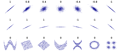
Several sets of (x, y) points, with the Pearson correlation coefficient of x and y for each set. Note that the correlation reflects the noisiness and direction of a linear relationship (top row), but not the slope of that relationship (middle), nor many aspects of nonlinear relationships (bottom). N.B.: the figure in the center has a slope of 0 but in that case the correlation coefficient is undefined because the variance of Y is zero.

Pearson's product-moment coefficient

The most familiar measure of dependence between two quantities is the Pearson product-moment correlation coefficient, or "Pearson's correlation coefficient", commonly called simply "the correlation coefficient". It is obtained by dividing the covariance of the two variables by the product of their standard deviations. Karl Pearson developed the coefficient from a similar but slightly different idea by Francis Galton.^[4]

The population correlation coefficient ρ_X,Y between two random variables X and Y with expected values μ_X and μ_Y and standard deviations σ_X and σ_Y is defined as

${\displaystyle \rho _{X,Y}=\mathrm {corr} (X,Y)={\mathrm {cov} (X,Y) \over \sigma _{X}\sigma _{Y}}={E[(X-\mu _{X})(Y-\mu _{Y})] \over \sigma _{X}\sigma _{Y}},}$

where E is the expected value operator, cov means covariance, and corr is a widely used alternative notation for the correlation coefficient.

The Pearson correlation is defined only if both of the standard deviations are finite and nonzero. It is a corollary of the Cauchy–Schwarz inequality that the correlation cannot exceed 1 in absolute value. The correlation coefficient is symmetric: corr(X,Y) = corr(Y,X).

The Pearson correlation is +1 in the case of a perfect direct (increasing) linear relationship (correlation), −1 in the case of a perfect decreasing (inverse) linear relationship (anticorrelation),^[5] and some value in the open interval (−1, 1) in all other cases, indicating the degree of linear dependence between the variables. As it approaches zero there is less of a relationship (closer to uncorrelated). The closer the coefficient is to either −1 or 1, the stronger the correlation between the variables.

If the variables are independent, Pearson's correlation coefficient is 0, but the converse is not true because the correlation coefficient detects only linear dependencies between two variables. For example, suppose the random variable X is symmetrically distributed about zero, and Y = X². Then Y is completely determined by X, so that X and Y are perfectly dependent, but their correlation is zero; they are uncorrelated. However, in the special case when X and Y are jointly normal, uncorrelatedness is equivalent to independence.

If we have a series of n measurements of X and Y written as x_i and y_i for i = 1, 2, ..., n, then the sample correlation coefficient can be used to estimate the population Pearson correlation r between X and Y. The sample correlation coefficient is written as

${\displaystyle r_{xy}={\frac {\sum \limits _{i=1}^{n}(x_{i}-{\bar {x}})(y_{i}-{\bar {y}})}{(n-1)s_{x}s_{y}}}={\frac {\sum \limits _{i=1}^{n}(x_{i}-{\bar {x}})(y_{i}-{\bar {y}})}{\sqrt {\sum \limits _{i=1}^{n}(x_{i}-{\bar {x}})^{2}\sum \limits _{i=1}^{n}(y_{i}-{\bar {y}})^{2}}}},}$

where x and y are the sample means of X and Y, and s_x and s_y are the corrected sample standard deviations of X and Y.

The uncorrected form of r (not standard) can be written as

${\displaystyle {\begin{aligned}r_{xy}&={\frac {\sum x_{i}y_{i}-n{\bar {x}}{\bar {y}}}{ns_{x}s_{y}}}\\&={\frac {n\sum x_{i}y_{i}-\sum x_{i}\sum y_{i}}{{\sqrt {n\sum x_{i}^{2}-(\sum x_{i})^{2}}}~{\sqrt {n\sum y_{i}^{2}-(\sum y_{i})^{2}}}}}.\end{aligned}}}$

where s_x and s_y are now the uncorrected sample standard deviations of X and Y.

If x and y are results of measurements that contain measurement error, the realistic limits on the correlation coefficient are not −1 to +1 but a smaller range.^[6] For the case of a linear model with a single independent variable, the coefficient of determination (R squared) is the square of r, Pearson's product-moment coefficient.

Rank correlation coefficients

Rank correlation coefficients, such as Spearman's rank correlation coefficient and Kendall's rank correlation coefficient (τ) measure the extent to which, as one variable increases, the other variable tends to increase, without requiring that increase to be represented by a linear relationship. If, as the one variable increases, the other decreases, the rank correlation coefficients will be negative. It is common to regard these rank correlation coefficients as alternatives to Pearson's coefficient, used either to reduce the amount of calculation or to make the coefficient less sensitive to non-normality in distributions. However, this view has little mathematical basis, as rank correlation coefficients measure a different type of relationship than the Pearson product-moment correlation coefficient, and are best seen as measures of a different type of association, rather than as alternative measure of the population correlation coefficient.^[7][8]

To illustrate the nature of rank correlation, and its difference from linear correlation, consider the following four pairs of numbers (x, y):

(0, 1), (10, 100), (101, 500), (102, 2000).

As we go from each pair to the next pair x increases, and so does y. This relationship is perfect, in the sense that an increase in x is always accompanied by an increase in y. This means that we have a perfect rank correlation, and both Spearman's and Kendall's correlation coefficients are 1, whereas in this example Pearson product-moment correlation coefficient is 0.7544, indicating that the points are far from lying on a straight line. In the same way if y always decreases when x increases, the rank correlation coefficients will be −1, while the Pearson product-moment correlation coefficient may or may not be close to −1, depending on how close the points are to a straight line. Although in the extreme cases of perfect rank correlation the two coefficients are both equal (being both +1 or both −1), this is not generally the case, and so values of the two coefficients cannot meaningfully be compared.^[7] For example, for the three pairs (1, 1) (2, 3) (3, 2) Spearman's coefficient is 1/2, while Kendall's coefficient is 1/3.

Other measures of dependence among random variables

The information given by a correlation coefficient is not enough to define the dependence structure between random variables.^[9] The correlation coefficient completely defines the dependence structure only in very particular cases, for example when the distribution is a multivariate normal distribution. (See diagram above.) In the case of elliptical distributions it characterizes the (hyper-)ellipses of equal density; however, it does not completely characterize the dependence structure (for example, a multivariate t-distribution's degrees of freedom determine the level of tail dependence).
Distance correlation^[10][11] was introduced to address the deficiency of Pearson's correlation that it can be zero for dependent random variables; zero distance correlation implies independence.

The Randomized Dependence Coefficient^[12] is a computationally efficient, copula-based measure of dependence between multivariate random variables. RDC is invariant with respect to non-linear scalings of random variables, is capable of discovering a wide range of functional association patterns and takes value zero at independence.

The correlation ratio is able to detect almost any functional dependency,^{[citation needed][clarification needed]} and the entropy-based mutual information, total correlation and dual total correlation are capable of detecting even more general dependencies. These are sometimes referred to as multi-moment correlation measures,^{[citation needed]} in comparison to those that consider only second moment (pairwise or quadratic) dependence.

The polychoric correlation is another correlation applied to ordinal data that aims to estimate the correlation between theorised latent variables.

One way to capture a more complete view of dependence structure is to consider a copula between them.

The coefficient of determination generalizes the correlation coefficient for relationships beyond simple linear regression.

Sensitivity to the data distribution

The degree of dependence between variables X and Y does not depend on the scale on which the variables are expressed. That is, if we are analyzing the relationship between X and Y, most correlation measures are unaffected by transforming X to a + bX and Y to c + dY, where a, b, c, and d are constants (b and d being positive). This is true of some correlation statistics as well as their population analogues. Some correlation statistics, such as the rank correlation coefficient, are also invariant to monotone transformations of the marginal distributions of X and/or Y.

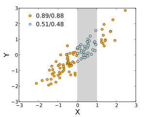
Pearson/Spearman correlation coefficients between X and Y are shown when the two variables' ranges are unrestricted, and when the range of X is restricted to the interval (0,1).

Most correlation measures are sensitive to the manner in which X and Y are sampled. Dependencies tend to be stronger if viewed over a wider range of values. Thus, if we consider the correlation coefficient between the heights of fathers and their sons over all adult males, and compare it to the same correlation coefficient calculated when the fathers are selected to be between 165 cm and 170 cm in height, the correlation will be weaker in the latter case. Several techniques have been developed that attempt to correct for range restriction in one or both variables, and are commonly used in meta-analysis; the most common are Thorndike's case II and case III equations.^[13]

Various correlation measures in use may be undefined for certain joint distributions of X and Y. For example, the Pearson correlation coefficient is defined in terms of moments, and hence will be undefined if the moments are undefined. Measures of dependence based on quantiles are always defined. Sample-based statistics intended to estimate population measures of dependence may or may not have desirable statistical properties such as being unbiased, or asymptotically consistent, based on the spatial structure of the population from which the data were sampled.

Sensitivity to the data distribution can be used to an advantage. For example, scaled correlation is designed to use the sensitivity to the range in order to pick out correlations between fast components of time series.^[14] By reducing the range of values in a controlled manner, the correlations on long time scale are filtered out and only the correlations on short time scales are revealed.

Correlation matrices

"Correlation matrix" redirects here. For correlation matrices in quantum physics, see Quark–lepton complementarity.

The correlation matrix of n random variables X₁, ..., X_n is the n × n matrix whose i,j entry is corr(X_i, X_j). If the measures of correlation used are product-moment coefficients, the correlation matrix is the same as the covariance matrix of the standardized random variables ${\displaystyle X_{i}/\sigma (X_{i})}$ for ${\displaystyle i=1,\dots ,n}$. This applies both to the matrix of population correlations (in which case σ is the population standard deviation), and to the matrix of sample correlations (in which case σ denotes the sample standard deviation). Consequently, each is necessarily a positive-semidefinite matrix. Moreover, the correlation matrix is strictly positive definite if no variable can have all its values exactly generated as a linear function of the values of the others.

The correlation matrix is symmetric because the correlation between X_i and X_j is the same as the correlation between X_j and X_i.

A correlation matrix appears, for example, in one formula for the coefficient of multiple determination, a measure of goodness of fit in multiple regression.

Common misconceptions

Correlation and causality

The conventional dictum that "correlation does not imply causation" means that correlation cannot be used to infer a causal relationship between the variables.^[15] This dictum should not be taken to mean that correlations cannot indicate the potential existence of causal relations. However, the causes underlying the correlation, if any, may be indirect and unknown, and high correlations also overlap with identity relations (tautologies), where no causal process exists. Consequently, establishing a correlation between two variables is not a sufficient condition to establish a causal relationship (in either direction).

A correlation between age and height in children is fairly causally transparent, but a correlation between mood and health in people is less so. Does improved mood lead to improved health, or does good health lead to good mood, or both? Or does some other factor underlie both? In other words, a correlation can be taken as evidence for a possible causal relationship, but cannot indicate what the causal relationship, if any, might be.

Correlation and linearity

Four sets of data with the same correlation of 0.816

The Pearson correlation coefficient indicates the strength of a linear relationship between two variables, but its value generally does not completely characterize their relationship.^[16] In particular, if the conditional mean of Y given X, denoted E(Y | X), is not linear in X, the correlation coefficient will not fully determine the form of E(Y | X).

The image on the right shows scatter plots of Anscombe's quartet, a set of four different pairs of variables created by Francis Anscombe.^[17] The four y variables have the same mean (7.5), variance (4.12), correlation (0.816) and regression line (y = 3 + 0.5x). However, as can be seen on the plots, the distribution of the variables is very different. The first one (top left) seems to be distributed normally, and corresponds to what one would expect when considering two variables correlated and following the assumption of normality. The second one (top right) is not distributed normally; while an obvious relationship between the two variables can be observed, it is not linear. In this case the Pearson correlation coefficient does not indicate that there is an exact functional relationship: only the extent to which that relationship can be approximated by a linear relationship. In the third case (bottom left), the linear relationship is perfect, except for one outlier which exerts enough influence to lower the correlation coefficient from 1 to 0.816. Finally, the fourth example (bottom right) shows another example when one outlier is enough to produce a high correlation coefficient, even though the relationship between the two variables is not linear.

These examples indicate that the correlation coefficient, as a summary statistic, cannot replace visual examination of the data. Note that the examples are sometimes said to demonstrate that the Pearson correlation assumes that the data follow a normal distribution, but this is not correct.^[4]

Bivariate normal distribution

If a pair (X, Y) of random variables follows a bivariate normal distribution, the conditional mean E(X|Y) is a linear function of Y, and the conditional mean E(Y|X) is a linear function of X. The correlation coefficient r between X and Y, along with the marginal means and variances of X and Y, determines this linear relationship:

${\displaystyle E(Y\mid X)=E(Y)+r\sigma _{y}{\frac {X-E(X)}{\sigma _{x}}},}$

where ${\displaystyle E(X)}$ and ${\displaystyle E(Y)}$ are the expected values of X and Y, respectively, and σ_x and σ_y are the standard deviations of X and Y, respectively.

Set theory

From Wikipedia, the free encyclopedia

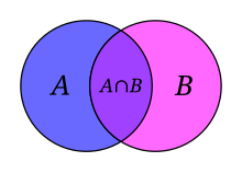
A Venn diagram illustrating the intersection of two sets.

Set theory is a branch of mathematical logic that studies sets, which informally are collections of objects. Although any type of object can be collected into a set, set theory is applied most often to objects that are relevant to mathematics. The language of set theory can be used in the definitions of nearly all mathematical objects.

The modern study of set theory was initiated by Georg Cantor and Richard Dedekind in the 1870s. After the discovery of paradoxes in naive set theory, such as Russell's paradox, numerous axiom systems were proposed in the early twentieth century, of which the Zermelo–Fraenkel axioms, with or without the axiom of choice, are the best-known.

Set theory is commonly employed as a foundational system for mathematics, particularly in the form of Zermelo–Fraenkel set theory with the axiom of choice. Beyond its foundational role, set theory is a branch of mathematics in its own right, with an active research community. Contemporary research into set theory includes a diverse collection of topics, ranging from the structure of the real number line to the study of the consistency of large cardinals.

History

Georg Cantor.

Mathematical topics typically emerge and evolve through interactions among many researchers. Set theory, however, was founded by a single paper in 1874 by Georg Cantor: "On a Property of the Collection of All Real Algebraic Numbers".^[1][2]

Since the 5th century BC, beginning with Greek mathematician Zeno of Elea in the West and early Indian mathematicians in the East, mathematicians had struggled with the concept of infinity. Especially notable is the work of Bernard Bolzano in the first half of the 19th century.^[3] Modern understanding of infinity began in 1870–1874 and was motivated by Cantor's work in real analysis.^[4] An 1872 meeting between Cantor and Richard Dedekind influenced Cantor's thinking and culminated in Cantor's 1874 paper.

Cantor's work initially polarized the mathematicians of his day. While Karl Weierstrass and Dedekind supported Cantor, Leopold Kronecker, now seen as a founder of mathematical constructivism, did not. Cantorian set theory eventually became widespread, due to the utility of Cantorian concepts, such as one-to-one correspondence among sets, his proof that there are more real numbers than integers, and the "infinity of infinities" ("Cantor's paradise") resulting from the power set operation. This utility of set theory led to the article "Mengenlehre" contributed in 1898 by Arthur Schoenflies to Klein's encyclopedia.

The next wave of excitement in set theory came around 1900, when it was discovered that some interpretations of Cantorian set theory gave rise to several contradictions, called antinomies or paradoxes. Bertrand Russell and Ernst Zermelo independently found the simplest and best known paradox, now called Russell's paradox: consider "the set of all sets that are not members of themselves", which leads to a contradiction since it must be a member of itself and not a member of itself. In 1899 Cantor had himself posed the question "What is the cardinal number of the set of all sets?", and obtained a related paradox. Russell used his paradox as a theme in his 1903 review of continental mathematics in his The Principles of Mathematics.

In 1906 English readers gained the book Theory of Sets of Points^[5] by husband and wife William Henry Young and Grace Chisholm Young, published by Cambridge University Press.

The momentum of set theory was such that debate on the paradoxes did not lead to its abandonment. The work of Zermelo in 1908 and the work of Abraham Fraenkel and Thoralf Skolem in 1922 resulted in the set of axioms ZFC, which became the most commonly used set of axioms for set theory. The work of analysts such as Henri Lebesgue demonstrated the great mathematical utility of set theory, which has since become woven into the fabric of modern mathematics. Set theory is commonly used as a foundational system, although in some areas-such as algebraic geometry and algebraic topology-category theory is thought to be a preferred foundation.

Basic concepts and notation

Set theory begins with a fundamental binary relation between an object o and a set A. If o is a member (or element) of A, the notation o ∈ A is used. Since sets are objects, the membership relation can relate sets as well.

A derived binary relation between two sets is the subset relation, also called set inclusion. If all the members of set A are also members of set B, then A is a subset of B, denoted A ⊆ B. For example, {1, 2} is a subset of {1, 2, 3} , and so is {2} but {1, 4} is not. As insinuated from this definition, a set is a subset of itself. For cases where this possibility is unsuitable or would make sense to be rejected, the term proper subset is defined. A is called a proper subset of B if and only if A is a subset of B, but A is not equal to B. Note also that 1, 2, and 3 are members (elements) of the set {1, 2, 3} but are not subsets of it; and in turn, the subsets, such as {1}, are not members of the set {1, 2, 3}.

Just as arithmetic features binary operations on numbers, set theory features binary operations on sets. The:

• Union of the sets A and B, denoted A ∪ B, is the set of all objects that are a member of A, or B, or both. The union of {1, 2, 3} and {2, 3, 4} is the set {1, 2, 3, 4} .
• Intersection of the sets A and B, denoted A ∩ B, is the set of all objects that are members of both A and B. The intersection of {1, 2, 3} and {2, 3, 4} is the set {2, 3} .
• Set difference of U and A, denoted U \ A, is the set of all members of U that are not members of A. The set difference {1, 2, 3} \ {2, 3, 4} is {1} , while, conversely, the set difference {2, 3, 4} \ {1, 2, 3} is {4} . When A is a subset of U, the set difference U \ A is also called the complement of A in U. In this case, if the choice of U is clear from the context, the notation A^c is sometimes used instead of U \ A, particularly if U is a universal set as in the study of Venn diagrams.
• Symmetric difference of sets A and B, denoted A △ B or A ⊖ B, is the set of all objects that are a member of exactly one of A and B (elements which are in one of the sets, but not in both). For instance, for the sets {1, 2, 3} and {2, 3, 4} , the symmetric difference set is {1, 4} . It is the set difference of the union and the intersection, (A ∪ B) \ (A ∩ B) or (A \ B) ∪ (B \ A).
• Cartesian product of A and B, denoted A × B, is the set whose members are all possible ordered pairs (a, b) where a is a member of A and b is a member of B. The cartesian product of {1, 2} and {red, white} is {(1, red), (1, white), (2, red), (2, white)}.
• Power set of a set A is the set whose members are all of the possible subsets of A. For example, the power set of {1, 2} is { {}, {1}, {2}, {1, 2} } .

Some basic sets of central importance are the empty set (the unique set containing no elements; occasionally called the null set though this name is ambiguous), the set of natural numbers, and the set of real numbers.

Some ontology

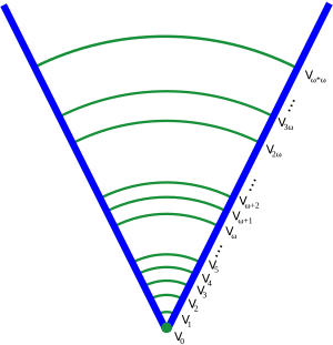
An initial segment of the von Neumann hierarchy.

A set is pure if all of its members are sets, all members of its members are sets, and so on. For example, the set {{}} containing only the empty set is a nonempty pure set. In modern set theory, it is common to restrict attention to the von Neumann universe of pure sets, and many systems of axiomatic set theory are designed to axiomatize the pure sets only. There are many technical advantages to this restriction, and little generality is lost, because essentially all mathematical concepts can be modeled by pure sets. Sets in the von Neumann universe are organized into a cumulative hierarchy, based on how deeply their members, members of members, etc. are nested. Each set in this hierarchy is assigned (by transfinite recursion) an ordinal number α, known as its rank. The rank of a pure set X is defined to be the least upper bound of all successors of ranks of members of X. For example, the empty set is assigned rank 0, while the set {{}} containing only the empty set is assigned rank 1. For each ordinal α, the set V_α is defined to consist of all pure sets with rank less than α. The entire von Neumann universe is denoted V.

Axiomatic set theory

Elementary set theory can be studied informally and intuitively, and so can be taught in primary schools using Venn diagrams. The intuitive approach tacitly assumes that a set may be formed from the class of all objects satisfying any particular defining condition. This assumption gives rise to paradoxes, the simplest and best known of which are Russell's paradox and the Burali-Forti paradox. Axiomatic set theory was originally devised to rid set theory of such paradoxes.^[6]

The most widely studied systems of axiomatic set theory imply that all sets form a cumulative hierarchy. Such systems come in two flavors, those whose ontology consists of:

• Sets alone. This includes the most common axiomatic set theory, Zermelo–Fraenkel set theory (ZFC), which includes the axiom of choice. Fragments of ZFC include:
  • Zermelo set theory, which replaces the axiom schema of replacement with that of separation;
  • General set theory, a small fragment of Zermelo set theory sufficient for the Peano axioms and finite sets;
  • Kripke–Platek set theory, which omits the axioms of infinity, powerset, and choice, and weakens the axiom schemata of separation and replacement.
• Sets and proper classes. These include Von Neumann–Bernays–Gödel set theory, which has the same strength as ZFC for theorems about sets alone, and Morse–Kelley set theory and Tarski–Grothendieck set theory, both of which are stronger than ZFC.

The above systems can be modified to allow urelements, objects that can be members of sets but that are not themselves sets and do not have any members.

The systems of New Foundations NFU (allowing urelements) and NF (lacking them) are not based on a cumulative hierarchy. NF and NFU include a "set of everything, " relative to which every set has a complement. In these systems urelements matter, because NF, but not NFU, produces sets for which the axiom of choice does not hold.

Systems of constructive set theory, such as CST, CZF, and IZF, embed their set axioms in intuitionistic instead of classical logic. Yet other systems accept classical logic but feature a nonstandard membership relation. These include rough set theory and fuzzy set theory, in which the value of an atomic formula embodying the membership relation is not simply True or False. The Boolean-valued models of ZFC are a related subject.

An enrichment of ZFC called internal set theory was proposed by Edward Nelson in 1977.

Applications

Many mathematical concepts can be defined precisely using only set theoretic concepts. For example, mathematical structures as diverse as graphs, manifolds, rings, and vector spaces can all be defined as sets satisfying various (axiomatic) properties. Equivalence and order relations are ubiquitous in mathematics, and the theory of mathematical relations can be described in set theory.

Set theory is also a promising foundational system for much of mathematics. Since the publication of the first volume of Principia Mathematica, it has been claimed that most or even all mathematical theorems can be derived using an aptly designed set of axioms for set theory, augmented with many definitions, using first or second order logic. For example, properties of the natural and real numbers can be derived within set theory, as each number system can be identified with a set of equivalence classes under a suitable equivalence relation whose field is some infinite set.

Set theory as a foundation for mathematical analysis, topology, abstract algebra, and discrete mathematics is likewise uncontroversial; mathematicians accept that (in principle) theorems in these areas can be derived from the relevant definitions and the axioms of set theory. Few full derivations of complex mathematical theorems from set theory have been formally verified, however, because such formal derivations are often much longer than the natural language proofs mathematicians commonly present. One verification project, Metamath, includes human-written, computer‐verified derivations of more than 12,000 theorems starting from ZFC set theory, first order logic and propositional logic.

Areas of study

Set theory is a major area of research in mathematics, with many interrelated subfields.

Combinatorial set theory

Combinatorial set theory concerns extensions of finite combinatorics to infinite sets. This includes the study of cardinal arithmetic and the study of extensions of Ramsey's theorem such as the Erdős–Rado theorem.

Descriptive set theory

Descriptive set theory is the study of subsets of the real line and, more generally, subsets of Polish spaces. It begins with the study of pointclasses in the Borel hierarchy and extends to the study of more complex hierarchies such as the projective hierarchy and the Wadge hierarchy. Many properties of Borel sets can be established in ZFC, but proving these properties hold for more complicated sets requires additional axioms related to determinacy and large cardinals.

The field of effective descriptive set theory is between set theory and recursion theory. It includes the study of lightface pointclasses, and is closely related to hyperarithmetical theory. In many cases, results of classical descriptive set theory have effective versions; in some cases, new results are obtained by proving the effective version first and then extending ("relativizing") it to make it more broadly applicable.

A recent area of research concerns Borel equivalence relations and more complicated definable equivalence relations. This has important applications to the study of invariants in many fields of mathematics.

Fuzzy set theory

In set theory as Cantor defined and Zermelo and Fraenkel axiomatized, an object is either a member of a set or not. In fuzzy set theory this condition was relaxed by Lotfi A. Zadeh so an object has a degree of membership in a set, a number between 0 and 1. For example, the degree of membership of a person in the set of "tall people" is more flexible than a simple yes or no answer and can be a real number such as 0.75.

Inner model theory

An inner model of Zermelo–Fraenkel set theory (ZF) is a transitive class that includes all the ordinals and satisfies all the axioms of ZF. The canonical example is the constructible universe L developed by Gödel. One reason that the study of inner models is of interest is that it can be used to prove consistency results. For example, it can be shown that regardless of whether a model V of ZF satisfies the continuum hypothesis or the axiom of choice, the inner model L constructed inside the original model will satisfy both the generalized continuum hypothesis and the axiom of choice. Thus the assumption that ZF is consistent (has at least one model) implies that ZF together with these two principles is consistent.

The study of inner models is common in the study of determinacy and large cardinals, especially when considering axioms such as the axiom of determinacy that contradict the axiom of choice. Even if a fixed model of set theory satisfies the axiom of choice, it is possible for an inner model to fail to satisfy the axiom of choice. For example, the existence of sufficiently large cardinals implies that there is an inner model satisfying the axiom of determinacy (and thus not satisfying the axiom of choice).^[7]

Large cardinals

A large cardinal is a cardinal number with an extra property. Many such properties are studied, including inaccessible cardinals, measurable cardinals, and many more. These properties typically imply the cardinal number must be very large, with the existence of a cardinal with the specified property unprovable in Zermelo-Fraenkel set theory.

Determinacy

Determinacy refers to the fact that, under appropriate assumptions, certain two-player games of perfect information are determined from the start in the sense that one player must have a winning strategy. The existence of these strategies has important consequences in descriptive set theory, as the assumption that a broader class of games is determined often implies that a broader class of sets will have a topological property. The axiom of determinacy (AD) is an important object of study; although incompatible with the axiom of choice, AD implies that all subsets of the real line are well behaved (in particular, measurable and with the perfect set property). AD can be used to prove that the Wadge degrees have an elegant structure.

Forcing

Paul Cohen invented the method of forcing while searching for a model of ZFC in which the continuum hypothesis fails, or a model of ZF in which the axiom of choice fails. Forcing adjoins to some given model of set theory additional sets in order to create a larger model with properties determined (i.e. "forced") by the construction and the original model. For example, Cohen's construction adjoins additional subsets of the natural numbers without changing any of the cardinal numbers of the original model. Forcing is also one of two methods for proving relative consistency by finitistic methods, the other method being Boolean-valued models.

Cardinal invariants

A cardinal invariant is a property of the real line measured by a cardinal number. For example, a well-studied invariant is the smallest cardinality of a collection of meagre sets of reals whose union is the entire real line. These are invariants in the sense that any two isomorphic models of set theory must give the same cardinal for each invariant. Many cardinal invariants have been studied, and the relationships between them are often complex and related to axioms of set theory.

Set-theoretic topology

Set-theoretic topology studies questions of general topology that are set-theoretic in nature or that require advanced methods of set theory for their solution. Many of these theorems are independent of ZFC, requiring stronger axioms for their proof. A famous problem is the normal Moore space question, a question in general topology that was the subject of intense research. The answer to the normal Moore space question was eventually proved to be independent of ZFC.

Objections to set theory as a foundation for mathematics

From set theory's inception, some mathematicians have objected to it as a foundation for mathematics. The most common objection to set theory, one Kronecker voiced in set theory's earliest years, starts from the constructivist view that mathematics is loosely related to computation. If this view is granted, then the treatment of infinite sets, both in naive and in axiomatic set theory, introduces into mathematics methods and objects that are not computable even in principle. The feasibility of constructivism as a substitute foundation for mathematics was greatly increased by Errett Bishop's influential book Foundations of Constructive Analysis.^[8]

A different objection put forth by Henri Poincaré is that defining sets using the axiom schemas of specification and replacement, as well as the axiom of power set, introduces impredicativity, a type of circularity, into the definitions of mathematical objects. The scope of predicatively founded mathematics, while less than that of the commonly accepted Zermelo-Fraenkel theory, is much greater than that of constructive mathematics, to the point that Solomon Feferman has said that "all of scientifically applicable analysis can be developed [using predicative methods]".^[9]

Ludwig Wittgenstein condemned set theory. He wrote that "set theory is wrong", since it builds on the "nonsense" of fictitious symbolism, has "pernicious idioms", and that it is nonsensical to talk about "all numbers".^[10] Wittgenstein's views about the foundations of mathematics were later criticised by Georg Kreisel and Paul Bernays, and investigated by Crispin Wright, among others.

Category theorists have proposed topos theory as an alternative to traditional axiomatic set theory. Topos theory can interpret various alternatives to that theory, such as constructivism, finite set theory, and computable set theory.^[11][12] Topoi also give a natural setting for forcing and discussions of the independence of choice from ZF, as well as providing the framework for pointless topology and Stone spaces.^[13]

An active area of research is the univalent foundations and related to it homotopy type theory. Here, sets may be defined as certain kinds of types, with universal properties of sets arising from higher inductive types. Principles such as the axiom of choice and the law of the excluded middle appear in a spectrum of different forms, some of which can be proven, others which correspond to the classical notions; this allows for a detailed discussion of the effect of these axioms on mathematics.^[14][15]