Search This Blog

Sunday, May 3, 2015

Quantum electrodynamics


From Wikipedia, the free encyclopedia

In particle physics, quantum electrodynamics (QED) is the relativistic quantum field theory of electrodynamics.

In essence, it describes how light and matter interact and is the first theory where full agreement between quantum mechanics and special relativity is achieved. QED mathematically describes all phenomena involving electrically charged particles interacting by means of exchange of photons and represents the quantum counterpart of classical electromagnetism giving a complete account of matter and light interaction.

In technical terms, QED can be described as a perturbation theory of the electromagnetic quantum vacuum. Richard Feynman called it "the jewel of physics" for its extremely accurate predictions of quantities like the anomalous magnetic moment of the electron and the Lamb shift of the energy levels of hydrogen.[1]:Ch1

History


The first formulation of a quantum theory describing radiation and matter interaction is attributed to British scientist Paul Dirac, who (during the 1920s) was first able to compute the coefficient of spontaneous emission of an atom.[2]

Dirac described the quantization of the electromagnetic field as an ensemble of harmonic oscillators with the introduction of the concept of creation and annihilation operators of particles. In the following years, with contributions from Wolfgang Pauli, Eugene Wigner, Pascual Jordan, Werner Heisenberg and an elegant formulation of quantum electrodynamics due to Enrico Fermi,[3] physicists came to believe that, in principle, it would be possible to perform any computation for any physical process involving photons and charged particles. However, further studies by Felix Bloch with Arnold Nordsieck,[4] and Victor Weisskopf,[5] in 1937 and 1939, revealed that such computations were reliable only at a first order of perturbation theory, a problem already pointed out by Robert Oppenheimer.[6] At higher orders in the series infinities emerged, making such computations meaningless and casting serious doubts on the internal consistency of the theory itself. With no solution for this problem known at the time, it appeared that a fundamental incompatibility existed between special relativity and quantum mechanics.

Difficulties with the theory increased through the end of 1940. Improvements in microwave technology made it possible to take more precise measurements of the shift of the levels of a hydrogen atom,[7] now known as the Lamb shift and magnetic moment of the electron.[8] These experiments unequivocally exposed discrepancies which the theory was unable to explain.

A first indication of a possible way out was given by Hans Bethe. In 1947, while he was traveling by train to reach Schenectady from New York,[9] after giving a talk at the conference at Shelter Island on the subject, Bethe completed the first non-relativistic computation of the shift of the lines of the hydrogen atom as measured by Lamb and Retherford.[10] Despite the limitations of the computation, agreement was excellent. The idea was simply to attach infinities to corrections of mass and charge that were actually fixed to a finite value by experiments. In this way, the infinities get absorbed in those constants and yield a finite result in good agreement with experiments. This procedure was named renormalization.

Feynman (center) and Oppenheimer (right) at Los Alamos.

Based on Bethe's intuition and fundamental papers on the subject by Sin-Itiro Tomonaga,[11] Julian Schwinger,[12][13] Richard Feynman[14][15][16] and Freeman Dyson,[17][18] it was finally possible to get fully covariant formulations that were finite at any order in a perturbation series of quantum electrodynamics. Sin-Itiro Tomonaga, Julian Schwinger and Richard Feynman were jointly awarded with a Nobel prize in physics in 1965 for their work in this area.[19] Their contributions, and those of Freeman Dyson, were about covariant and gauge invariant formulations of quantum electrodynamics that allow computations of observables at any order of perturbation theory. Feynman's mathematical technique, based on his diagrams, initially seemed very different from the field-theoretic, operator-based approach of Schwinger and Tomonaga, but Freeman Dyson later showed that the two approaches were equivalent.[17] Renormalization, the need to attach a physical meaning at certain divergences appearing in the theory through integrals, has subsequently become one of the fundamental aspects of quantum field theory and has come to be seen as a criterion for a theory's general acceptability. Even though renormalization works very well in practice, Feynman was never entirely comfortable with its mathematical validity, even referring to renormalization as a "shell game" and "hocus pocus".[1]:128

QED has served as the model and template for all subsequent quantum field theories. One such subsequent theory is quantum chromodynamics, which began in the early 1960s and attained its present form in the 1975 work by H. David Politzer, Sidney Coleman, David Gross and Frank Wilczek. Building on the pioneering work of Schwinger, Gerald Guralnik, Dick Hagen, and Tom Kibble,[20][21] Peter Higgs, Jeffrey Goldstone, and others, Sheldon Glashow, Steven Weinberg and Abdus Salam independently showed how the weak nuclear force and quantum electrodynamics could be merged into a single electroweak force.

Feynman's view of quantum electrodynamics

Introduction

Near the end of his life, Richard P. Feynman gave a series of lectures on QED intended for the lay public. These lectures were transcribed and published as Feynman (1985), QED: The strange theory of light and matter,[1] a classic non-mathematical exposition of QED from the point of view articulated below.

The key components of Feynman's presentation of QED are three basic actions.[1]:85
  • A photon goes from one place and time to another place and time.
  • An electron goes from one place and time to another place and time.
  • An electron emits or absorbs a photon at a certain place and time.
These actions are represented in a form of visual shorthand by the three basic elements of Feynman diagrams: a wavy line for the photon, a straight line for the electron and a junction of two straight lines and a wavy one for a vertex representing emission or absorption of a photon by an electron.

It is important not to over-interpret these diagrams. Nothing is implied about how a particle gets from one point to another. The diagrams do not imply that the particles are moving in straight or curved lines. They do not imply that the particles are moving with fixed speeds. The fact that the photon is often represented, by convention, by a wavy line and not a straight one does not imply that it is thought that it is more wavelike than is an electron. The images are just symbols to represent the actions above: photons and electrons do, somehow, move from point to point and electrons, somehow, emit and absorb photons. We do not know how these things happen, but the theory tells us about the probabilities of these things happening.

As well as the visual shorthand for the actions Feynman introduces another kind of shorthand for the numerical quantities called probability amplitudes. The probability is the square of the total probability amplitude. If a photon moves from one place and time—in shorthand, A—to another place and time—in shorthand, B—the associated quantity is written in Feynman's shorthand as P(A to B). The similar quantity for an electron moving from C to D is written E(C to D). The quantity which tells us about the probability amplitude for the emission or absorption of a photon he calls 'j'. This is related to, but not the same as, the measured electron charge 'e'.[1]:91

QED is based on the assumption that complex interactions of many electrons and photons can be represented by fitting together a suitable collection of the above three building blocks, and then using the probability amplitudes to calculate the probability of any such complex interaction. It turns out that the basic idea of QED can be communicated while making the assumption that the square of the total of the probability amplitudes mentioned above (P(A to B), E(A to B) and 'j') acts just like our everyday probability. (A simplification made in Feynman's book.) Later on, this will be corrected to include specifically quantum-style mathematics, following Feynman.

The basic rules of probability amplitudes that will be used are that a) if an event can happen in a variety of different ways then its probability amplitude is the sum of the probability amplitudes of the possible ways and b) if a process involves a number of independent sub-processes then its probability amplitude is the product of the component probability amplitudes.[1]:93

Basic constructions

Suppose we start with one electron at a certain place and time (this place and time being given the arbitrary label A) and a photon at another place and time (given the label B). A typical question from a physical standpoint is: 'What is the probability of finding an electron at C (another place and a later time) and a photon at D (yet another place and time)?'. The simplest process to achieve this end is for the electron to move from A to C (an elementary action) and for the photon to move from B to D (another elementary action). From a knowledge of the probability amplitudes of each of these sub-processes – E(A to C) and P(B to D) – then we would expect to calculate the probability amplitude of both happening together by multiplying them, using rule b) above. This gives a simple estimated overall probability amplitude, which is squared to give an estimated probability.

But there are other ways in which the end result could come about. The electron might move to a place and time E where it absorbs the photon; then move on before emitting another photon at F; then move on to C where it is detected, while the new photon moves on to D. The probability of this complex process can again be calculated by knowing the probability amplitudes of each of the individual actions: three electron actions, two photon actions and two vertexes – one emission and one absorption. We would expect to find the total probability amplitude by multiplying the probability amplitudes of each of the actions, for any chosen positions of E and F. We then, using rule a) above, have to add up all these probability amplitudes for all the alternatives for E and F. (This is not elementary in practice, and involves integration.) But there is another possibility, which is that the electron first moves to G where it emits a photon which goes on to D, while the electron moves on to H, where it absorbs the first photon, before moving on to C. Again we can calculate the probability amplitude of these possibilities (for all points G and H). We then have a better estimation for the total probability amplitude by adding the probability amplitudes of these two possibilities to our original simple estimate. Incidentally the name given to this process of a photon interacting with an electron in this way is Compton scattering.

There are an infinite number of other intermediate processes in which more and more photons are absorbed and/or emitted. For each of these possibilities there is a Feynman diagram describing it. This implies a complex computation for the resulting probability amplitudes, but provided it is the case that the more complicated the diagram the less it contributes to the result, it is only a matter of time and effort to find as accurate an answer as one wants to the original question. This is the basic approach of QED. To calculate the probability of any interactive process between electrons and photons it is a matter of first noting, with Feynman diagrams, all the possible ways in which the process can be constructed from the three basic elements. Each diagram involves some calculation involving definite rules to find the associated probability amplitude.

That basic scaffolding remains when one moves to a quantum description but some conceptual changes are needed. One is that whereas we might expect in our everyday life that there would be some constraints on the points to which a particle can move, that is not true in full quantum electrodynamics. There is a possibility of an electron at A, or a photon at B, moving as a basic action to any other place and time in the universe. That includes places that could only be reached at speeds greater than that of light and also earlier times. (An electron moving backwards in time can be viewed as a positron moving forward in time.)[1]:89, 98–99

Probability amplitudes


Feynman replaces complex numbers with spinning arrows, which start at emission and end at detection of a particle. The sum of all resulting arrows represents the total probability of the event. In this diagram, light emitted by the source S bounces off a few segments of the mirror (in blue) before reaching the detector at P. The sum of all paths must be taken into account. The graph below depicts the total time spent to traverse each of the paths above.

Quantum mechanics introduces an important change in the way probabilities are computed. Probabilities are still represented by the usual real numbers we use for probabilities in our everyday world, but probabilities are computed as the square of probability amplitudes. Probability amplitudes are complex numbers.

Feynman avoids exposing the reader to the mathematics of complex numbers by using a simple but accurate representation of them as arrows on a piece of paper or screen. (These must not be confused with the arrows of Feynman diagrams which are actually simplified representations in two dimensions of a relationship between points in three dimensions of space and one of time.) The amplitude arrows are fundamental to the description of the world given by quantum theory. No satisfactory reason has been given for why they are needed. But pragmatically we have to accept that they are an essential part of our description of all quantum phenomena. They are related to our everyday ideas of probability by the simple rule that the probability of an event is the square of the length of the corresponding amplitude arrow. So, for a given process, if two probability amplitudes, v and w, are involved, the probability of the process will be given either by
P=|\mathbf{v}+\mathbf{w}|^2
or
P=|\mathbf{v} \,\mathbf{w}|^2.
The rules as regards adding or multiplying, however, are the same as above. But where you would expect to add or multiply probabilities, instead you add or multiply probability amplitudes that now are complex numbers.

Addition of probability amplitudes as complex numbers

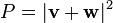
Addition and multiplication are familiar operations in the theory of complex numbers and are given in the figures. The sum is found as follows. Let the start of the second arrow be at the end of the first. The sum is then a third arrow that goes directly from the start of the first to the end of the second. The product of two arrows is an arrow whose length is the product of the two lengths. The direction of the product is found by adding the angles that each of the two have been turned through relative to a reference direction: that gives the angle that the product is turned relative to the reference direction.

That change, from probabilities to probability amplitudes, complicates the mathematics without changing the basic approach. But that change is still not quite enough because it fails to take into account the fact that both photons and electrons can be polarized, which is to say that their orientations in space and time have to be taken into account. Therefore P(A to B) actually consists of 16 complex numbers, or probability amplitude arrows.[1]:120–121 There are also some minor changes to do with the quantity "j", which may have to be rotated by a multiple of 90° for some polarizations, which is only of interest for the detailed bookkeeping.

Associated with the fact that the electron can be polarized is another small necessary detail which is connected with the fact that an electron is a fermion and obeys Fermi–Dirac statistics. The basic rule is that if we have the probability amplitude for a given complex process involving more than one electron, then when we include (as we always must) the complementary Feynman diagram in which we just exchange two electron events, the resulting amplitude is the reverse – the negative – of the first. The simplest case would be two electrons starting at A and B ending at C and D. The amplitude would be calculated as the "difference", E(A to D) × E(B to C) − E(A to C) × E(B to D), where we would expect, from our everyday idea of probabilities, that it would be a sum.[1]:112–113

Propagators

Finally, one has to compute P (A to B) and E (C to D) corresponding to the probability amplitudes for the photon and the electron respectively. These are essentially the solutions of the Dirac Equation which describes the behavior of the electron's probability amplitude and the Klein–Gordon equation which describes the behavior of the photon's probability amplitude. These are called Feynman propagators. The translation to a notation commonly used in the standard literature is as follows:
P(\mbox{A to B}) \rightarrow D_F(x_B-x_A),\quad  E(\mbox{C to D}) \rightarrow S_F(x_D-x_C)
where a shorthand symbol such as x_A stands for the four real numbers which give the time and position in three dimensions of the point labeled A.

Mass renormalization


A problem arose historically which held up progress for twenty years: although we start with the assumption of three basic "simple" actions, the rules of the game say that if we want to calculate the probability amplitude for an electron to get from A to B we must take into account all the possible ways: all possible Feynman diagrams with those end points. Thus there will be a way in which the electron travels to C, emits a photon there and then absorbs it again at D before moving on to B. Or it could do this kind of thing twice, or more. In short we have a fractal-like situation in which if we look closely at a line it breaks up into a collection of "simple" lines, each of which, if looked at closely, are in turn composed of "simple" lines, and so on ad infinitum. This is a very difficult situation to handle. If adding that detail only altered things slightly then it would not have been too bad, but disaster struck when it was found that the simple correction mentioned above led to infinite probability amplitudes. In time this problem was "fixed" by the technique of renormalization. However, Feynman himself remained unhappy about it, calling it a "dippy process".[1]:128

Conclusions

Within the above framework physicists were then able to calculate to a high degree of accuracy some of the properties of electrons, such as the anomalous magnetic dipole moment. However, as Feynman points out, it fails totally to explain why particles such as the electron have the masses they do. "There is no theory that adequately explains these numbers. We use the numbers in all our theories, but we don't understand them – what they are, or where they come from. I believe that from a fundamental point of view, this is a very interesting and serious problem."[1]:152

Mathematics

Mathematically, QED is an abelian gauge theory with the symmetry group U(1). The gauge field, which mediates the interaction between the charged spin-1/2 fields, is the electromagnetic field. The QED Lagrangian for a spin-1/2 field interacting with the electromagnetic field is given by the real part of[22]:78
\mathcal{L}=\bar\psi(i\gamma^\mu D_\mu-m)\psi -\frac{1}{4}F_{\mu\nu}F^{\mu\nu}
where
 \gamma^\mu are Dirac matrices;
\psi a bispinor field of spin-1/2 particles (e.g. electronpositron field);
\bar\psi\equiv\psi^\dagger\gamma^0, called "psi-bar", is sometimes referred to as the Dirac adjoint;
D_\mu \equiv \partial_\mu+ieA_\mu+ieB_\mu \,\! 
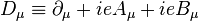
is the gauge covariant derivative;
e is the coupling constant, equal to the electric charge of the bispinor field;
Aμ is the covariant four-potential of the electromagnetic field generated by the electron itself;
Bμ is the external field imposed by external source;
F_{\mu\nu} = \partial_\mu A_\nu - \partial_\nu A_\mu \,\! 
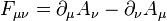
is the electromagnetic field tensor.

Equations of motion

To begin, substituting the definition of D into the Lagrangian gives us
\mathcal{L} = i \bar\psi \gamma^\mu \partial_\mu \psi - e\bar{\psi}\gamma_\mu (A^\mu+B^\mu) \psi -m \bar{\psi} \psi - \frac{1}{4}F_{\mu\nu}F^{\mu\nu}. \,
Next, we can substitute this Lagrangian into the Euler–Lagrange equation of motion for a field:
 \partial_\mu \left( \frac{\partial \mathcal{L}}{\partial ( \partial_\mu \psi )} \right) - \frac{\partial \mathcal{L}}{\partial \psi} = 0 \,


(2)
to find the field equations for QED.

The two terms from this Lagrangian are then
\partial_\mu \left( \frac{\partial \mathcal{L}}{\partial ( \partial_\mu \psi )} \right) = \partial_\mu \left( i \bar{\psi} \gamma^\mu \right), \,
\frac{\partial \mathcal{L}}{\partial \psi} = -e\bar{\psi}\gamma_\mu (A^\mu+B^\mu) - m \bar{\psi}. \,
Substituting these two back into the Euler–Lagrange equation (2) results in
i \partial_\mu \bar{\psi} \gamma^\mu + e\bar{\psi}\gamma_\mu (A^\mu+B^\mu) + m \bar{\psi} = 0 \,
with complex conjugate
i \gamma^\mu \partial_\mu \psi - e \gamma_\mu (A^\mu+B^\mu) \psi - m \psi = 0. \,
Bringing the middle term to the right-hand side transforms this second equation into
i \gamma^\mu \partial_\mu \psi - m \psi = e \gamma_\mu (A^\mu+B^\mu) \psi \,
The left-hand side is like the original Dirac equation and the right-hand side is the interaction with the electromagnetic field.

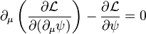
One further important equation can be found by substituting the above Lagrangian into another Euler–Lagrange equation, this time for the field, Aμ:
 \partial_\nu \left( \frac{\partial \mathcal{L}}{\partial ( \partial_\nu A_\mu )} \right) - \frac{\partial \mathcal{L}}{\partial A_\mu} = 0\,.


(3)
The two terms this time are
\partial_\nu \left( \frac{\partial \mathcal{L}}{\partial ( \partial_\nu A_\mu )} \right) = \partial_\nu \left( \partial^\mu A^\nu - \partial^\nu A^\mu \right), \,
\frac{\partial \mathcal{L}}{\partial A_\mu} = -e\bar{\psi} \gamma^\mu \psi \,
and these two terms, when substituted back into (3) give us
\partial_\nu F^{\nu \mu} = e \bar{\psi} \gamma^\mu \psi \,
Now, if we impose the Lorenz gauge condition, that the divergence of the four potential vanishes
\partial_{\mu} A^\mu = 0
then we get
\Box A^{\mu}=e\bar{\psi} \gamma^{\mu} \psi\,,
which is a wave equation for the four potential, the QED version of the classical Maxwell equations in the Lorenz gauge. (In the above equation, the square represents the D'Alembert operator.)

Interaction picture

This theory can be straightforwardly quantized by treating bosonic and fermionic sectors[clarification needed] as free.
This permits us to build a set of asymptotic states which can be used to start a computation of the probability amplitudes for different processes. In order to do so, we have to compute an evolution operator that, for a given initial state |i\rangle, will give a final state \langle f| in such a way to have[22]:5
M_{fi}=\langle f|U|i\rangle.
This technique is also known as the S-matrix. The evolution operator is obtained in the interaction picture where time evolution is given by the interaction Hamiltonian, which is the integral over space of the second term in the Lagrangian density given above:[22]:123
V=e\int d^3x\bar\psi\gamma^\mu\psi A_\mu
and so, one has[22]:86
U=T\exp\left[-\frac{i}{\hbar}\int_{t_0}^tdt'V(t')\right]
where T is the time ordering operator. This evolution operator only has meaning as a series, and what we get here is a perturbation series with the fine structure constant as the development parameter. This series is called the Dyson series.

Feynman diagrams

Despite the conceptual clarity of this Feynman approach to QED, almost no early textbooks follow him in their presentation. When performing calculations it is much easier to work with the Fourier transforms of the propagators. Quantum physics considers particle's momenta rather than their positions, and it is convenient to think of particles as being created or annihilated when they interact. Feynman diagrams then look the same, but the lines have different interpretations. The electron line represents an electron with a given energy and momentum, with a similar interpretation of the photon line. A vertex diagram represents the annihilation of one electron and the creation of another together with the absorption or creation of a photon, each having specified energies and momenta.

Using Wick theorem on the terms of the Dyson series, all the terms of the S-matrix for quantum electrodynamics can be computed through the technique of Feynman diagrams.
To these rules we must add a further one for closed loops that implies an integration on momenta \int d^4p/(2\pi)^4, since these internal ("virtual") particles are not constrained to any specific energy–momentum – even that usually required by special relativity (see this article for details). From them, computations of probability amplitudes are straightforwardly given. An example is Compton scattering, with an electron and a photon undergoing elastic scattering.

Renormalizability

Higher order terms can be straightforwardly computed for the evolution operator but these terms display diagrams containing the following simpler ones[22]:ch 10
that, being closed loops, imply the presence of diverging integrals having no mathematical meaning. To overcome this difficulty, a technique called renormalization has been devised, producing finite results in very close agreement with experiments. It is important to note that a criterion for theory being meaningful after renormalization is that the number of diverging diagrams is finite. In this case the theory is said to be renormalizable. The reason for this is that to get observables renormalized one needs a finite number of constants to maintain the predictive value of the theory untouched. This is exactly the case of quantum electrodynamics displaying just three diverging diagrams. This procedure gives observables in very close agreement with experiment as seen e.g. for electron gyromagnetic ratio.

Renormalizability has become an essential criterion for a quantum field theory to be considered as a viable one. All the theories describing fundamental interactions, except gravitation whose quantum counterpart is presently under very active research, are renormalizable theories.

Nonconvergence of series

An argument by Freeman Dyson shows that the radius of convergence of the perturbation series in QED is zero.[23] The basic argument goes as follows: if the coupling constant were negative, this would be equivalent to the Coulomb force constant being negative. This would "reverse" the electromagnetic interaction so that like charges would attract and unlike charges would repel. This would render the vacuum unstable against decay into a cluster of electrons on one side of the universe and a cluster of positrons on the other side of the universe. Because the theory is 'sick' for any negative value of the coupling constant, the series do not converge, but are an asymptotic series.

From a modern perspective, we say that QED is not well defined as a quantum field theory to arbitrarily high energy.[24] The coupling constant runs to infinity at finite energy, signalling a Landau pole. The problem is essentially that QED is not asymptotically free. This is one of the motivations for embedding QED within a Grand Unified Theory.

Introduction to gauge theory


From Wikipedia, the free encyclopedia

A gauge theory is a type of theory in physics. Modern physical theories, such as the theory of electromagnetism, describe the nature of reality in terms of fields, e.g., the electromagnetic field, the gravitational field, and fields for the electron and all other elementary particles. A general feature of these field theories is that the fundamental fields cannot be directly measured; however, there are observable quantities that can be measured experimentally, such as charges, energies, and velocities. In field theories, different configurations of the unobservable fields can result in identical observable quantities. A transformation from one such field configuration to another is called a gauge transformation;[1][2] the lack of change in the measurable quantities, despite the field being transformed, is a property called gauge invariance. Since any kind of invariance under a field transformation is considered a symmetry, gauge invariance is sometimes called gauge symmetry. Generally, any theory that has the property of gauge invariance is considered a gauge theory.

With the advent of quantum mechanics in the 1920s, and with successive advances in quantum field theory, the importance of gauge transformations has steadily grown. Gauge theories constrain the laws of physics, because all the changes induced by a gauge transformation have to cancel each other out when written in terms of observable quantities. Over the course of the 20th century, physicists gradually realized that all forces (fundamental interactions) arise from the constraints imposed by local gauge symmetries, in which case the transformations vary from point to point in space and time. Perturbative quantum field theory (usually employed for scattering theory) describes forces in terms of force-mediating particles called gauge bosons. The nature of these particles is determined by the nature of the gauge transformations. The culmination of these efforts is the Standard Model, a quantum field theory explaining all of the fundamental interactions except gravity.

History and importance

The earliest field theory having a gauge symmetry was Maxwell's formulation of electrodynamics in 1864. The importance of this symmetry remained unnoticed in the earliest formulations. Similarly unnoticed, Hilbert had derived Einstein's equations of general relativity by postulating a symmetry under any change of coordinates. Later Hermann Weyl, in an attempt to unify general relativity and electromagnetism, conjectured (incorrectly, as it turned out) that invariance under the change of scale or "gauge" (a term inspired by the various track gauges of railroads) might also be a local symmetry of general relativity. Although Weyl's choice of the gauge was incorrect, the name "gauge" stuck to the approach. After the development of quantum mechanics, Weyl, Fock and London modified their gauge choice by replacing the scale factor with a change of wave phase, and applying it successfully to electromagnetism. Gauge symmetry was generalized mathematically in 1954 by Chen Ning Yang and Robert Mills in an attempt to describe the strong nuclear forces. This idea, dubbed Yang-Mills, later found application in the quantum field theory of the weak force, and its unification with electromagnetism in the electroweak theory.

The importance of gauge theories for physics stems from their tremendous success in providing a unified framework to describe the quantum-mechanical behavior of electromagnetism, the weak force and the strong force.
This gauge theory, known as the Standard Model, accurately describes experimental predictions regarding three of the four fundamental forces of nature.

In classical physics

Electromagnetism

Historically, the first example of gauge symmetry to be discovered was classical electromagnetism. A static electric field can be described in terms of an electric potential (voltage) that is defined at every point in space, and in practical work it is conventional to take the Earth as a physical reference that defines the zero level of the potential, or ground. But only differences in potential are physically measurable, which is the reason that a voltmeter must have two probes, and can only report the voltage difference between them. Thus one could choose to define all voltage differences relative to some other standard, rather than the Earth, resulting in the addition of a constant offset.[4] If the potential V is a solution to Maxwell's equations then, after this gauge transformation, the new potential V \rightarrow V+C is also a solution to Maxwell's equations and no experiment can distinguish between these two solutions. In other words the laws of physics governing electricity and magnetism (that is, Maxwell equations) are invariant under gauge transformation.[5] That is, Maxwell's equations have a gauge symmetry.
Generalizing from static electricity to electromagnetism, we have a second potential, the magnetic vector potential A, which can also undergo gauge transformations. These transformations may be local. That is, rather than adding a constant onto V, one can add a function that takes on different values at different points in space and time. If A is also changed in certain corresponding ways, then the same E and B fields result. The detailed mathematical relationship between the fields E and B and the potentials V and A is given in the article Gauge fixing, along with the precise statement of the nature of the gauge transformation. The relevant point here is that the fields remain the same under the gauge transformation, and therefore Maxwell's equations are still satisfied.

Gauge symmetry is closely related to charge conservation. Suppose that there existed some process by which one could violate conservation of charge, at least temporarily, by creating a charge q at a certain point in space, 1, moving it to some other point 2, and then destroying it. We might imagine that this process was consistent with conservation of energy. We could posit a rule stating that creating the charge required an input of energy E1=qV1 and destroying it released E2=qV2, which would seem natural since qV measures the extra energy stored in the electric field because of the existence of a charge at a certain point. (There may also be energy associated, e.g., with the rest mass of the particle, but that is not relevant to the present argument.) Conservation of energy would be satisfied, because the net energy released by creation and destruction of the particle, qV2-qV1, would be equal to the work done in moving the particle from 1 to 2, qV2-qV1. But although this scenario salvages conservation of energy, it violates gauge symmetry. Gauge symmetry requires that the laws of physics be invariant under the transformation V \rightarrow V+C, which implies that no experiment should be able to measure the absolute potential, without reference to some external standard such as an electrical ground. But the proposed rules E1=qV1 and E2=qV2 for the energies of creation and destruction would allow an experimenter to determine the absolute potential, simply by checking how much energy input was required in order to create the charge q at a particular point in space. The conclusion is that if gauge symmetry holds, and energy is conserved, then charge must be conserved.[6]

The Cartesian coordinate grid on this square has been distorted by a coordinate transformation, so that there is a nonlinear relationship between the old (x,y) coordinates and the new ones. Einstein's equations of general relativity are still valid in the new coordinate system. Such changes of coordinate system are the gauge transformations of general relativity.

General relativity

As discussed above, the gauge transformations for classical (i.e., non-quantum mechanical) general relativity are arbitrary coordinate transformations.[7] (Technically, the transformations must be invertible, and both the transformation and its inverse must be smooth, in the sense of being differentiable an arbitrary number of times.)

An example of a symmetry in a physical theory: translation invariance

Some global symmetries under changes of coordinate predate both general relativity and the concept of a gauge. For example, translation invariance was introduced in the era of Galileo, who eliminated the Aristotelian concept that various places in space, such as the earth and the heavens, obeyed different physical rules.

Suppose, for example, that one observer examines the properties of a hydrogen atom on Earth, the other—on the Moon (or any other place in the universe), the observer will find that their hydrogen atoms exhibit completely identical properties. Again, if one observer had examined a hydrogen atom today and the other—100 years ago (or any other time in the past or in the future), the two experiments would again produce completely identical results. The invariance of the properties of a hydrogen atom with respect to the time and place where these properties were investigated is called translation invariance.

Recalling our two observers from different ages: the time in their experiments is shifted by 100 years. If the time when the older observer did the experiment was t, the time of the modern experiment is t+100 years. Both observers discover the same laws of physics. Because light from hydrogen atoms in distant galaxies may reach the earth after having traveled across space for billions of years, in effect one can do such observations covering periods of time almost all the way back to the Big Bang, and they show that the laws of physics have always been the same.

In other words, if in the theory we change the time t to t+100 years (or indeed any other time shift) the theoretical predictions do not change.[8]

Another example of a symmetry: the invariance of Einstein's field equation under arbitrary coordinate transformations

In Einstein's general relativity, coordinates like x, y, z, and t are not only "relative" in the global sense of translations like t \rightarrow t+C, rotations, etc., but become completely arbitrary, so that for example one can define an entirely new timelike coordinate according to some arbitrary rule such as t \rightarrow t+t^3/t_0^2, where t_0 has units of time, and yet Einstein's equations will have the same form.[7][9]

Invariance of the form of an equation under an arbitrary coordinate transformation is customarily referred to as general covariance and equations with this property are referred to as written in the covariant form. General covariance is a special case of gauge invariance.

Maxwell's equations can also be expressed in a generally covariant form, which is as invariant under general coordinate transformation as Einstein's field equation.

In quantum mechanics

Quantum electrodynamics

Until the advent of quantum mechanics, the only well known example of gauge symmetry was in electromagnetism, and the general significance of the concept was not fully understood. For example, it was not clear whether it was the fields E and B or the potentials V and A that were the fundamental quantities; if the former, then the gauge transformations could be considered as nothing more than a mathematical trick.

Aharonov–Bohm experiment


Double-slit diffraction and interference pattern

In quantum mechanics a particle, such as an electron, is also described as a wave. For example, if the double-slit experiment is performed with electrons, then a wave-like interference pattern is observed. The electron has the highest probability of being detected at locations where the parts of the wave passing through the two slits are in phase with one another, resulting in constructive interference. The frequency of the electron wave is related to the kinetic energy of an individual electron particle via the quantum-mechanical relation E = hf. If there are no electric or magnetic fields present in this experiment, then the electron's energy is constant, and, for example, there will be a high probability of detecting the electron along the central axis of the experiment, where by symmetry the two parts of the wave are in phase.

But now suppose that the electrons in the experiment are subject to electric or magnetic fields. For example, if an electric field was imposed on one side of the axis but not on the other, the results of the experiment would be affected. The part of the electron wave passing through that side oscillates at a different rate, since its energy has had −eV added to it, where −e is the charge of the electron and V the electrical potential. The results of the experiment will be different, because phase relationships between the two parts of the electron wave have changed, and therefore the locations of constructive and destructive interference will be shifted to one side or the other. It is the electric potential that occurs here, not the electric field, and this is a manifestation of the fact that it is the potentials and not the fields that are of fundamental significance in quantum mechanics.

Schematic of double-slit experiment in which Aharonov–Bohm effect can be observed: electrons pass through two slits, interfering at an observation screen, with the interference pattern shifted when a magnetic field B is turned on in the cylindrical solenoid, marked in blue on the diagram.

Explanation with potentials

It is even possible to have cases in which an experiment's results differ when the potentials are changed, even if no charged particle is ever exposed to a different field. One such example is the Aharonov–Bohm effect, shown in the figure.[10] In this example, turning on the solenoid only causes a magnetic field B to exist within the solenoid. But the solenoid has been positioned so that the electron cannot possibly pass through its interior. If one believed that the fields were the fundamental quantities, then one would expect that the results of the experiment would be unchanged. In reality, the results are different, because turning on the solenoid changed the vector potential A in the region that the electrons do pass through. Now that it has been established that it is the potentials V and A that are fundamental, and not the fields E and B, we can see that the gauge transformations, which change V and A, have real physical significance, rather than being merely mathematical artifacts.

Gauge invariance: the results of the experiments are independent of the choice of the gauge for the potentials

Note that in these experiments, the only quantity that affects the result is the difference in phase between the two parts of the electron wave. Suppose we imagine the two parts of the electron wave as tiny clocks, each with a single hand that sweeps around in a circle, keeping track of its own phase. Although this cartoon ignores some technical details, it retains the physical phenomena that are important here.[11] If both clocks are sped up by the same amount, the phase relationship between them is unchanged, and the results of experiments are the same. Not only that, but it is not even necessary to change the speed of each clock by a fixed amount. We could change the angle of the hand on each clock by a varying amount θ, where θ could depend on both the position in space and on time. This would have no effect on the result of the experiment, since the final observation of the location of the electron occurs at a single place and time, so that the phase shift in each electron's "clock" would be the same, and the two effects would cancel out. This is another example of a gauge transformation: it is local, and it does not change the results of experiments.

Summary

In summary, gauge symmetry attains its full importance in the context of quantum mechanics. In the application of quantum mechanics to electromagnetism, i.e., quantum electrodynamics, gauge symmetry applies to both electromagnetic waves and electron waves. These two gauge symmetries are in fact intimately related. If a gauge transformation θ is applied to the electron waves, for example, then one must also apply a corresponding transformation to the potentials that describe the electromagnetic waves.[12] Gauge symmetry is required in order to make quantum electrodynamics a renormalizable theory, i.e., one in which the calculated predictions of all physically measurable quantities are finite.

Types of gauge symmetries

The description of the electrons in the subsection above as little clocks is in effect a statement of the mathematical rules according to which the phases of electrons are to be added and subtracted: they are to be treated as ordinary numbers, except that in the case where the result of the calculation falls outside the range of 0≤θ<360 365="" 5="" a="" about="" algebraic="" allowed="" an="" angle="" another="" are="" around="" as="" be="" by="" circle.="" completely="" considered="" covers="" electron="" equivalent="" exactly="" except="" experiments="" for="" force="" formed="" have="" interference="" into="" is="" it="" mathematical="" numbers.="" of="" ordinary="" p="" patterns="" phase="" properties="" property="" putting="" range="" real="" same="" say="" statement="" structure="" testable="" that="" the="" this="" those="" to="" verified="" waves.="" way="" we="" which="" wrap-around="" wrap="">

In mathematical terminology, electron phases form an Abelian group under addition, called the circle group or U(1). "Abelian" means that addition commutes, so that θ + φ = φ + θ. Group means that addition associates and has an identity element, namely "0". Also, for every phase there exists an inverse such that the sum of a phase and its inverse is 0. Other examples of abelian groups are the integers under addition, 0, and negation, and the nonzero fractions under product, 1, and reciprocal.

Gauge fixing of a twisted cylinder.

As a way of visualizing the choice of a gauge, consider whether it is possible to tell if a cylinder has been twisted. If the cylinder has no bumps, marks, or scratches on it, we cannot tell. We could, however, draw an arbitrary curve along the cylinder, defined by some function θ(x), where x measures distance along the axis of the cylinder. Once this arbitrary choice (the choice of gauge) has been made, it becomes possible to detect it if someone later twists the cylinder.

In 1954, Chen Ning Yang and Robert Mills proposed to generalize these ideas to noncommutative groups. A noncommutative gauge group can describe a field that, unlike the electromagnetic field, interacts with itself. For example, general relativity states that gravitational fields have energy, and special relativity concludes that energy is equivalent to mass. Hence a gravitational field induces a further gravitational field. The nuclear forces also have this self-interacting property.

Gauge bosons

Surprisingly, gauge symmetry can give a deeper explanation for the existence of interactions, such as the electrical and nuclear interactions. This arises from a type of gauge symmetry relating to the fact that all particles of a given type are experimentally indistinguishable from one other. Imagine that Alice and Betty are identical twins, labeled at birth by bracelets reading A and B. Because the girls are identical, nobody would be able to tell if they had been switched at birth; the labels A and B are arbitrary, and can be interchanged. Such a permanent interchanging of their identities is like a global gauge symmetry. There is also a corresponding local gauge symmetry, which describes the fact that from one moment to the next, Alice and Betty could swap roles while nobody was looking, and nobody would be able to tell. If we observe that Mom's favorite vase is broken, we can only infer that the blame belongs to one twin or the other, but we cannot tell whether the blame is 100% Alice's and 0% Betty's, or vice versa. If Alice and Betty are in fact quantum-mechanical particles rather than people, then they also have wave properties, including the property of superposition, which allows waves to be added, subtracted, and mixed arbitrarily. It follows that we are not even restricted to a complete swaps of identity. For example, if we observe that a certain amount of energy exists in a certain location in space, there is no experiment that can tell us whether that energy is 100% A's and 0% B's, 0% A's and 100% B's, or 20% A's and 80% B's, or some other mixture. The fact that the symmetry is local means that we cannot even count on these proportions to remain fixed as the particles propagate through space. The details of how this is represented mathematically depend on technical issues relating to the spins of the particles, but for our present purposes we consider a spinless particle, for which it turns out that the mixing can be specified by some arbitrary choice of gauge θ(x), where an angle θ = 0° represents 100% A and 0% B, θ = 90° means 0% A and 100% B, and intermediate angles represent mixtures.

According to the principles of quantum mechanics, particles do not actually have trajectories through space. Motion can only be described in terms of waves, and the momentum p of an individual particle is related to its wavelength λ by p = h/λ. In terms of empirical measurements, the wavelength can only be determined by observing a change in the wave between one point in space and another nearby point (mathematically, by differentiation). A wave with a shorter wavelength oscillates more rapidly, and therefore changes more rapidly between nearby points. Now suppose that we arbitrarily fix a gauge at one point in space, by saying that the energy at that location is 20% A's and 80% B's. We then measure the two waves at some other, nearby point, in order to determine their wavelengths.
But there are two entirely different reasons that the waves could have changed. They could have changed because they were oscillating with a certain wavelength, or they could have changed because the gauge function changed from a 20-80 mixture to, say, 21-79. If we ignore the second possibility, the resulting theory doesn't work; strange discrepancies in momentum will show up, violating the principle of conservation of momentum. Something in the theory must be changed.

Again there are technical issues relating to spin, but in several important cases, including electrically charged particles and particles interacting via nuclear forces, the solution to the problem is to impute physical reality to the gauge function θ(x). We say that if the function θ oscillates, it represents a new type of quantum-mechanical wave, and this new wave has its own momentum p = h/λ, which turns out to patch up the discrepancies that otherwise would have broken conservation of momentum. In the context of electromagnetism, the particles A and B would be charged particles such as electrons, and the quantum mechanical wave represented by θ would be the electromagnetic field. (Here we ignore the technical issues raised by the fact that electrons actually have spin 1/2, not spin zero. This oversimplification is the reason that the gauge field θ comes out to be a scalar, whereas the electromagnetic field is actually represented by a vector consisting of V and A.) The result is that we have an explanation for the presence of electromagnetic interactions: if we try to construct a gauge-symmetric theory of identical, non-interacting particles, the result is not self-consistent, and can only be repaired by adding electrical and magnetic fields that cause the particles to interact.

Although the function θ(x) describes a wave, the laws of quantum mechanics require that it also have particle properties. In the case of electromagnetism, the particle corresponding to electromagnetic waves is the photon. In general, such particles are called gauge bosons, where the term "boson" refers to a particle with integer spin. In the simplest versions of the theory, gauge bosons are massless, but it is also possible to construct versions in which they have mass, as is the case for the gauge bosons that transmit the nuclear decay forces.

Citation signal

From Wikipedia, the free encyclopedia https://en.wikipedia.org/wiki/Cit...