Search This Blog

Wednesday, February 3, 2016

Global warming too weak to be a theory


Mr. Peterman's Jan. 31 opinion piece on Mr. Pandelidis' guest column (Dec. 29) is interesting and deserves some analysis. He takes Mr. Pandelidis to task regarding the IPCC composition (politicians and bureaucrats vs. scientists). The IPCC is the Intergovernmental Panel on Climate Change, not the Interscientific Panel on Climate Change. Although the Working Groups are composed and led by scientists, their final product is shaped by government apparatchiks. Considering how many column-inches newspapers devote to this topic, it is clear climate change moved a long time ago from scientific debate in peer-reviewed publications to political debate with strident voices.But let’s back up a bit. The IPCC’s charter from the outset has been ”to assess on a comprehensive, objective, open and transparent basis the scientific, technical and socio-economic information relevant to understanding the scientific basis of risk of human-induced climate change, its potential impacts and options for adaptation and mitigation.” The IPCC (more accurately: the research community) is not looking significantly at natural variability causes, and given the full-court research press on human-induced factors, research monies are wanting in that area. The climate has always changed, and it has been both hotter and cooler in the past before the rise of mankind’s industry. It would be good to know why. Considering we are exiting from the Little Ice Age, it is not surprising things are warming.

The debate is the degree to which anthropogenic forces stack up against natural forces. That debate is far from settled. The significant slowdown over the last 18 years in global average temperature increases, despite over one-fifth of all human CO2 ever emitted going into the atmosphere, is fostering increasing doubt on the General Circulation Models (GCMs) used to underpin the IPCC conclusions.

This was noted in the final draft of the most recent Assessment Report (AR5) Summary for Policy Makers (SPM) of the IPCC:  “Models do not generally reproduce the observed reduction in surface warming trend over the last 10-15 years.” Unfortunately, when government representatives (vs. the scientists) released the final SPM, this language was removed. And Mr. Peterman wonders about Mr. Pandelidis’ skepticism?

Mr. Peterman goes on about the hypothesis of climate change (I would suggest the evidence is too weak to term it a theory) and Arrhenius. While the basic physics of the greenhouse effect are well understood, the modeled effect on the climate requires the introduction of feedback loops and amplification, notably water vapor.  Some of these feedbacks are poorly understood.  Consider the language by Working Group 1 of AR5: ”The assessed literature suggests that the range of climate sensitivities and transient responses covered by CMIP3/5 cannot be narrowed significantly by constraining the models with observations of the mean climate and variability, consistent with the difficulty of constraining the cloud feedbacks from observations. ”

Translation: despite significant expenditure of resources, we cannot further narrow climate sensitivities (that is, the change in temperature in response to various forcing factors) and still don’t understand clouds. In fact, scientists are unsure on whether the feedback from clouds is positive or negative.

The climate models are increasingly diverging from the observed temperature record; they fail the engineering test of usability through a lack of validation and verification. From an engineering perspective, models behaving this way would be in the dustbin. Instead, we have zealots that want to reshape the regulatory state and energy economy on the basis of such shabby models. Unbelievable.

Tuesday, February 2, 2016

Climate Change: The Burden of Proof


This article is based on a Heartland Panel talk [Dec7, 2015, at Hotel California, Paris].

The Intergovernmental Panel on Climate Change (IPCC) has to provide proof for significant human-caused climate change; yet their climate models have never been validated and are rapidly diverging from actual observations.  The real threat to humanity comes not from any (trivial) greenhouse warming but from cooling periods creating food shortages and famines.
-->

Burden of proof

Climate change has been going on for millions of years -- long before humans existed on this planet.  Obviously, the causes were all of natural origin and not anthropogenic.  There is no reason to think that these natural causes have suddenly stopped.  For example, volcanic eruptions, various types of solar influences, and atmosphere-ocean oscillations all continue today.   We cannot model these natural climate-forcings precisely and therefore cannot anticipate what they will be in the future.

But let’s call this the “Null hypothesis.” Logically therefore, the burden of proof falls upon alarmists to demonstrate that this null hypothesis is not adequate to account for empirical climate data.  In other words, alarmists must provide convincing observational evidence for anthropogenic climate change (ACC).  They must do this by detailed comparison of the data with climate models.  This is of course extremely difficult and virtually impossible since one cannot specify these natural influences precisely.

We’re not aware of such detailed comparisons, only of anecdotal evidence -- although we must admit that ACC is plausible; after all, CO2 is a greenhouse gas and its level has been rising mainly because of the burning of fossil fuels. 

Yet when we compare greenhouse models to past observations (“hindcasting”), it appears that ACC is much smaller than predicted by the models.  There’s even a time interval of no significant warming (“pause” or “hiatus”) during the past 18 years or so -- in spite of rapidly rising atmospheric CO2 levels. 

There seems to be at present no generally accepted explanation for this discrepancy between models and observations, mainly during the 21st century.  The five IPCC reports [1900 to 2014] insist that there is no “gap.”  Yet strangely, as this gap grows larger and larger, their claimed certainty that there is no gap becomes ever greater.  Successive IPCC reports give 50%, 66%, 90%, 95%, and 99% for this certainty.
[after J. Christy]

Needless to say, there are no sufficient conditions to establish the existence of any significant ACC from existing data.  Even necessary conditions based on empirical data, like temperature vs altitude and latitude, cloud cover, precipitation, are difficult to establish.
To summarize, any major disagreement of data with models therefore disproves ACC.

IPCC’s models are not validated -- and therefore not policy-relevant

In other words, GH models have not been validated and may never be validated -- and therefore are not policy-relevant.
Anyway, any warming observed during the past century appears to be trivially small and most likely economically beneficial overall.  Careful studies by leading economists and agricultural experts have established these facts [see for example NIPCC-ClimateChangeReconsidered-II – 2014].
[after J D’Aleo]

I therefore regard the absence of any significant GH warming as settled; note my emphasis on the word “significant.”  Policies to limit CO2 emissions are wasting resources that could better be used for genuine societal problems like public health.  They are also counter-productive since CO2 promotes plant growth and crop yields, as shown by dozens of agricultural publications. 

Surviving a coming climate cooling

I am much more concerned by a cooling climate -- as predicted by many climate scientists -- with its adverse effects on ecology and severe consequences for humanity.

Singer and Avery in “Unstoppable Global Warming: Every 1500 years” have described one form of observed cyclical climate change.  It was first seen during the past glaciation.  Loehle and Singer claim evidence for these cycles to extend into the present.

In particular, historical records identify the recent cycle of a (beneficial) Medieval Warm Period (MWP) and the (destructive) Little Ice Age (LIA) with its failed harvests, starvation, disease, and mass deaths.  Many solar experts predict another LIA cooling within decades. 
[after R. Alley]

I have therefore explored ways to counter the (imminent) next cooling phase through low-cost and low- ecological-risk geo-engineering, using a specific greenhouse effect – not based on CO2. 
At the same time, assuming that our scheme does not work perfectly, we need to prepare for adaptation to a colder climate, with special attention to supply of food and sustainable water and energy.

The outlook for such adaptation appears promising – provided there is adequate preparation.  However, the coming cold period will test the survivability of our technological civilization.

Monday, February 1, 2016

The Four Errors in Mann et al’s “The Likelihood of Recent Record Warmth”


Michael E. Mann and four others published the peer-reviewed paper “The Likelihood of Recent Record Warmth” in Nature: Scientific Reports (DOI: 10.1038/srep19831). I shall call this authors of this paper “Mann” for ease. Mann concludes (emphasis original):
We find that individual record years and the observed runs of record-setting temperatures were extremely unlikely to have occurred in the absence of human-caused climate change, though not nearly as unlikely as press reports have suggested. These same record temperatures were, by contrast, quite likely to have occurred in the presence of anthropogenic climate forcing.
This is confused and, in part, in error, as I show below. I am anxious people understand that Mann’s errors are in no way unique or rare; indeed, they are banal and ubiquitous. I therefore hope this article serves as a primer in how not to analyze time series.

First Error

Suppose you want to guess the height of the next person you meet when going outdoors. This value is uncertain, and so we can use probability to quantify our uncertainty in its value. Suppose as a crude approximation we used a normal distribution (it’s crude because we can only measure height to positive, finite, discrete levels and the normal allows numbers on the real line). The normal is characterized by two parameters, a location and spread. Next suppose God Himself told us that the values of these parameters were 5’5″ and 1’4″. We are thus as certain as possible in the value of these parameters. But are we as certain in the height of the next person? Can we, for instance, claim there is a 100% chance the next person will be, no matter what, 5’5″?

Obviously not. All we can say are things like this: “Given our model and God’s word on the value of the parameters, we are about 90% sure the next person’s height will be between 3’3″ and 7’7″.” (Don’t forget children are persons, too. The strange upper range is odd because the normal is, as advertised, crude. But it does not matter which model is used: my central argument remains.)

What kind of mistake would be it to claim that the next person will be for certain 5’5″? Whatever name you give this, it is the first error which pervades Mann’s paper.

The temperature values (anomalies) they use are presented as if they are certain, when in fact they are the estimates of a parameter of some probability model. Nobody knows that the temperature anomaly was precisely -0.10 in 1920 (or whatever value was claimed). Since this anomaly was the result of a probability model, to say we know it precisely is just like saying we know the exact height will be certainly 5’5″. Therefore, every temperature (or anomaly) that is used by Mann must, but does not, come equipped with a measure of its uncertainty.

We want the predictive uncertainty, as in the height example, and not the parametric uncertainty, which would only show the plus-or-minus in the model’s parameter value for temperature. In the height example, we didn’t have any uncertainty in the parameter because we received the value from on High. But if God only told us the central parameter was 5’5″ +/- 3″, then the uncertainty we have in the next height must widen—and by a lot—to take this extra uncertainty into account. The same is true for temperatures/anomalies.

Therefore, every graph and calculation in Mann’s paper which uses the temperatures/anomalies as if they were certain is wrong. In Mann’s favor, absolutely everybody makes the same error as they. This, however, is no excuse. An error repeated does not become a truth.

Nevertheless, I, like Mann and everybody else, will assume that this magnificent, non-ignorable, and thesis-destroying error does not exist. I will treat the temperatures/anomalies as if they are certain. This trick does not fix the other errors, which I will now show.

Second Error

You are in Las Vegas watching a craps game. On the come out, a player throws a “snake eyes” (a pair of ones). Given what we know about dice (they have six sides, one of which must show, etc.) the probability of snake eyes is 1/36. The next player (because the first crapped out) opens also with snake eyes. The probability of this is also 1/36.

Now what, given what we know of dice, is the probability of two snake eyes in a row? Well, this is 1/36 * 1/36 = 1/1296. This is a small number, about 0.0008. Because it is less than the magic number in statistics, does that mean the casino is cheating and causing the dice to come up snake eyes? Or can “chance” explain this?

First notice that in each throw, some things caused each total, i.e. various physical forces caused the dice to land the way they did. The players at the table did not know these causes. But a physicist might: he might measure the gravitional field, the spin (in three dimensions) of the dice as they left the players’ hands, the momentum given the dice by the throwers, the elasticity of table, the friction of the tablecloth, and so forth. If the physicist could measure these forces, he would be able to predict what the dice would do. The better he knows the forces, the better he could predict. If he knew the forces precisely he could predict the outcome with certainty. (This is why Vegas bans contrivances to measure forces/causes.)

From this it follows that “chance” did not cause the dice totals. Chance is not a physical force, and since it has no ontological being, it cannot be an efficient cause. Chance is thus a product of our ignorance of forces. Chance, then, is a synonym for probability. And probability is not a cause.

This means it is improper to ask, as most do ask, “What is the chance of snake eyes?” There is no single chance: the question has no proper answer. Why? Because the chance calculated depends on the information assumed. The bare question “What is the chance” does not tell us what information to assume, therefore it cannot be answered.

To the player, who knows only the possible totals of the dice, the chance is 1/36. To the physicist who measured all the causes, it is 1. To a second physicist who could only measure partial causes, the chance would be north of 1/36, but south of 1, depending on how the measurements were probative of the dice total. And so forth.

We have two players in a row shooting snake eyes. And we have calculated, from the players’ perspective, i.e. using their knowledge, the chance of this occurring. But we could have also asked, “Given only our knowledge of dice totals etc., what are the chances of seeing two snake eyes in a row in a sequence of N tosses?” N can be 2, 3, 100, 1000, any number we like. Because N can vary, the chance calculated will vary. That leads to the natural question: what is the right N to use for the Vegas example?

The answer is: there is no right N. The N picked depends on the situation we want to consider. It depends on decisions somebody makes. What might these decisions be? Anything. To the craps player who only has $20 to risk, N will be small. To the casino, it will be large. And so on.

Why is this important? Because the length of some sequence we happen to observe is not inherently of interest in and of itself. Whatever N is, it is still the case that some thing or things caused the values of the sequence. The probabilities we calculate cannot eliminate cause. Therefore, we have to be extremely cautious in interpreting the chance of any sequence, because (a) the probabilities we calculate depend on the sequence’s length and the length of interest depends on decisions somebody makes, and (b) in no case does cause somehow disappear the larger or smaller N is.

The second error Mann makes, and an error which is duplicated far and wide, is to assume that probability has any bearing on cause. We want to know what caused the temperatures/anomalies to take the values they did. Probability is of no help in this. Yet Mann assumes because the probability of a sequence calculated conditional on one set of information is different from the probability of the same sequence calculated conditional on another set of information, that therefore the only possible cause of the sequence (or of part of it) is thus global warming. This is the fallacy of the false dichotomy. The magnitude and nature of this error is discussed next.

The fallacy of the false dichotomy in the dice example is now plain. Because the probability of the observed N = 2 sequence of snake eyes was low given the information only about dice totals, it does not follow that therefore the casino cheated. Notice that, assuming the casino did cheat, the probability of two snake eyes is high (or even 1, assuming the casino had perfect control). We cannot compare these two probabilities, 0.0008 and 1, and conclude that “chance” could not have been a cause, therefore cheating must have.

And the same is true in temperature/anomaly sequences, as we shall now see.

Third Error

Put all this another way: suppose N is a temperature/anomaly series of which a physicist knows the cause of every value. What, given the physicist’s knowledge, is the chance of this sequence? It is 1. Why? Because it is no different than the dice throws: if we know the cause, we can predict with certainty. But what if we don’t know the cause? That is an excellent question.

What is the probability of a temperature/anomaly sequence where we do not know the cause? Answer: there is none. Why? Because since all probability is conditional on the knowledge assumed, if we do not assume anything no probability can be calculated. Obviously, the sequence happened, therefore it was caused. But absent knowledge of cause, and not assuming anything else like we did arbitrarily in the height example or as was natural in the case of dice totals, we must remain silent on probability.

Suppose we assume, arbitrarily, only that anomalies can only take the values -1 to 1 in increments of 0.01. That makes 201 possible anomalies. Given only this information, what is the probability the next anomaly takes the value, say, 0? It is 1/201. Suppose in fact we observe the next anomaly to be 0, and further suppose the anomaly after that is also 0. What are the chances of two 0s in a row? In a sequence of N = 2, and given only our arbitrary assumption, it is 1/201 * 1/201 = 1/40401. This is also less than the magic number. Is it thus the case that Nature “cheated” and made two 0s in a row?

Well, yes, in the sense that Nature causes all anomalies (and assuming, as is true, we are part of Nature). But this answer doesn’t quite capture the gist of the question. Before we come to that, assume, also arbitrarily, that a different set of information, say that the uncertainty in the temperatures/anomalies is represented by a more complex probability model (our first arbitrary assumption was also a probability model). Let this more complex probability model be an autoregressive moving-average, or ARMA, model. Now this model has certain parameters, but assume we know what these are.

Given this ARMA, what is the probability of two 0s in a row? It will be some number. It is not of the least importance what this number is. Why? For the same reason the 1/40401 was of no interest. And it’s the same reason any probability calculated from any probability model is of no interest to answer questions of cause.

Look at it this way. All probability models are silent on cause. And cause is what we want to know. But if we can’t know cause, and don’t forget we’re assuming we don’t know the cause of our temperature/anomaly sequence, we can at least quantify our uncertainty in a sequence conditional on some probability model. But since we’re assuming the probability model, the probabilities it spits out are the probabilities it spits out. They do not and cannot prove the goodness or badness of the model assumption. And they cannot be used to claim some thing other than “chance” is the one and only cause: that’s the fallacy of the false dichotomy. If we assume the model we have is good, for whatever reason, then whatever the probability of the sequence it gives, the sequence must still have been caused, and this model wasn’t the cause. Just like in the dice example, where the probability of two snake eyes, according to our simple model, were low. That low probability did not prove, one way or the other, that the casino cheated.

Mann calls the the casino not cheating the “null hypothesis”. Or rather, their “null hypothesis” is that his ARMA model (they actually created several) caused the anomaly sequence, with the false dichotomy alternate hypothesis that global warming was the only other (partial) cause. This, we now see, is wrong. All the calculations Mann provides to show probabilities of the sequence under any assumption—one of their ARMA or one of their concocted CMIP5 “all-forcing experiments”—have no bearing whatsoever on the only relevant physical question: What caused the sequence?

Fourth Error

It is true that global warming might be a partial cause of the anomaly sequence. Indeed, every working scientist assumes, what is almost a truism, that mankind has some effect on the climate. The only question is: how much? And the answer might be: only a trivial amount. Thus, it might also be true that global warming as a partial cause is ignorable for most questions or decisions made about values of temperature.

How can we tell? Only one way. Build causal or determinative models that has global warming as a component. Then make predictions of future values of temperature. If these predictions match (how to match is important question I here ignore), then we have good (but not complete) evidence that global warming is a cause. But if they do not match, we have good evidence that it isn’t.

Predictions of global temperature from models like CMIP, which are not shown in Mann, do not match the actual values of temperature, and haven’t for a long time. We therefore have excellent evidence that we do not understand all of the causes of global temperature and that global warming as it is represented in the models is in error.

Mann’s fourth error is to show how well the global-warming-assumption model can be made to fit past data. This fit is only of minor interest, because we could also get good fit with any number of probability models, and indeed Mann shows good fit for some of these models. But we know that probability models are silent on cause, therefore model fit is not indicative of cause either.

Conclusion

Calculations showing “There was an X% chance of this sequence” always assume what they set out to prove, and are thus of no interest whatsoever in assessing questions of cause. A casino can ask “Given the standard assumptions about dice, what is the chance of seeing N snake eyes in a row?” if, for whatever reason it has an interest in that question, but whatever the answer is, i.e. however small that probability is, it does not answer what causes the dice to land the way they do.

Consider that casinos are diligent in trying to understand cause. Dice throws are thus heavily regulated: they must hit a wall, the player may not do anything fancy with them (as pictured above), etc. When dice are old they are replaced, because wear indicates lack of symmetry and symmetry is important in cause. And so forth. It is only because casinos know that players do not know (or cannot manipulate) the causes of dice throws that they allow the game.

It is the job of physicists to understand the myriad causes of temperature sequences. Just like in the dice throw, there is not one cause, but many. And again like the dice throw, the more causes a physicist knows the better the predictions he will make. The opposite is also true: the fewer causes he knows, the worse the predictions he will make. And, given the poor performance of causal models over the last thirty years, we do not understand cause well.

The dice example differed from the temperature because with dice there was a natural (non-causal) probability model. We don’t have that with temperature, except to say we only know the possible values of anomalies (as the example above showed). Predictions can be made using this probability model, just like predictions of dice throws can be made with its natural probability model. Physical intuition argues these temperature predictions with this simple model won’t be very good. Therefore, if prediction is our goal, and it is a good goal, other probability models may be sought in the hope these will give better performance. As good as these predictions might be, no probability will tell us the cause of any sequence.

Because an assumed probability model said some sequence was rare, it does not mean the sequence was therefore caused by whatever mechanism that takes one’s fancy. You still have to do the hard work of proving the mechanism was the cause, and that it will be a cause into the future. That is shown by making good predictions. We are not there yet. And why, if you did know cause, would you employ some cheap and known-to-be-false probability model to argue an observed sequence had low probability—conditional on assuming this probability model is true?

Lastly, please don’t forget that everything that happened in Mann’s calculations, and in my examples after the First Error, are wrong because we do not know with certainty the values of the actual temperature/anomaly series. The probabilities we calculate for this series to take certain values can take the uncertainty we have in these past values into account, but it becomes complicated. That many don’t know how to do it is one reason the First Error is ubiquitous.

Tuesday, January 26, 2016

Hydrogen bond


From Wikipedia, the free encyclopedia


AFM image of napthalenetetracarboxylic diimide molecules on silver interacting via hydrogen bonding (77 K).[1]

Model of hydrogen bonds (1) between molecules of water

A hydrogen bond is the electrostatic attraction between polar groups that occurs when a hydrogen (H) atom bound to a highly electronegative atom such as nitrogen (N), oxygen (O) or fluorine (F) experiences attraction to some other nearby highly electronegative atom.

These hydrogen-bond attractions can occur between molecules (intermolecular) or within different parts of a single molecule (intramolecular).[2] Depending on geometry and environmental conditions, the hydrogen bond may be worth between 5 and 30 kJ/mole in thermodynamic terms. This makes it stronger than a van der Waals interaction, but weaker than covalent or ionic bonds. This type of bond can occur in inorganic molecules such as water and in organic molecules like DNA and proteins.

Intermolecular hydrogen bonding is responsible for the high boiling point of water (100 °C) compared to the other group 16 hydrides that have no hydrogen bonds. Intramolecular hydrogen bonding is partly responsible for the secondary and tertiary structures of proteins and nucleic acids. It also plays an important role in the structure of polymers, both synthetic and natural.

In 2011, an IUPAC Task Group recommended a modern evidence-based definition of hydrogen bonding, which was published in the IUPAC journal Pure and Applied Chemistry. This definition specifies that The hydrogen bond is an attractive interaction between a hydrogen atom from a molecule or a molecular fragment X–H in which X is more electronegative than H, and an atom or a group of atoms in the same or a different molecule, in which there is evidence of bond formation.[3] An accompanying detailed technical report provides the rationale behind the new definition.[4]

Bonding


An example of intermolecular hydrogen bonding in a self-assembled dimer complex reported by Meijer and coworkers.[5] The hydrogen bonds are represented by dotted lines.

Intramolecular hydrogen bonding in acetylacetone helps stabilize the enol tautomer.

A hydrogen atom attached to a relatively electronegative atom will play the role of the hydrogen bond donor.[6] This electronegative atom is usually fluorine, oxygen, or nitrogen. A hydrogen attached to carbon can also participate in hydrogen bonding when the carbon atom is bound to electronegative atoms, as is the case in chloroform, CHCl3.[7][8][9] An example of a hydrogen bond donor is the hydrogen from the hydroxyl group of ethanol, which is bonded to an oxygen.
An electronegative atom such as fluorine, oxygen, or nitrogen will be the hydrogen bond acceptor, whether or not it is bonded to a hydrogen atom. An example of a hydrogen bond acceptor that does not have a hydrogen atom bonded to it is the oxygen atom in diethyl ether.

Examples of hydrogen bond donating (donors) and hydrogen bond accepting groups (acceptors)

Cyclic dimer of acetic acid; dashed green lines represent hydrogen bonds

In the donor molecule, the electronegative atom attracts the electron cloud from around the hydrogen nucleus of the donor, and, by decentralizing the cloud, leaves the atom with a positive partial charge. Because of the small size of hydrogen relative to other atoms and molecules, the resulting charge, though only partial, represents a large charge density. A hydrogen bond results when this strong positive charge density attracts a lone pair of electrons on another heteroatom, which then becomes the hydrogen-bond acceptor.

The hydrogen bond is often described as an electrostatic dipole-dipole interaction. However, it also has some features of covalent bonding: it is directional and strong, produces interatomic distances shorter than the sum of the van der Waals radii, and usually involves a limited number of interaction partners, which can be interpreted as a type of valence. These covalent features are more substantial when acceptors bind hydrogens from more electronegative donors.

The partially covalent nature of a hydrogen bond raises the following questions: "To which molecule or atom does the hydrogen nucleus belong?" and "Which should be labeled 'donor' and which 'acceptor'?" Usually, this is simple to determine on the basis of interatomic distances in the X−HY system, where the dots represent the hydrogen bond: the X−H distance is typically ≈110 pm, whereas the HY distance is ≈160 to 200 pm. Liquids that display hydrogen bonding (such as water) are called associated liquids.

Hydrogen bonds can vary in strength from very weak (1–2 kJ mol−1) to extremely strong (161.5 kJ mol−1 in the ion HF
2
).[10][11] Typical enthalpies in vapor include:
  • F−H:F (161.5 kJ/mol or 38.6 kcal/mol)
  • O−H:N (29 kJ/mol or 6.9 kcal/mol)
  • O−H:O (21 kJ/mol or 5.0 kcal/mol)
  • N−H:N (13 kJ/mol or 3.1 kcal/mol)
  • N−H:O (8 kJ/mol or 1.9 kcal/mol)
  • HO−H:OH+
    3
    (18 kJ/mol[12] or 4.3 kcal/mol; data obtained using molecular dynamics as detailed in the reference and should be compared to 7.9 kJ/mol for bulk water, obtained using the same molecular dynamics.)
Quantum chemical calculations of the relevant interresidue potential constants (compliance constants) revealed[how?] large differences between individual H bonds of the same type. For example, the central interresidue N−H···N hydrogen bond between guanine and cytosine is much stronger in comparison to the N−H···N bond between the adenine-thymine pair.[13]

The length of hydrogen bonds depends on bond strength, temperature, and pressure. The bond strength itself is dependent on temperature, pressure, bond angle, and environment (usually characterized by local dielectric constant). The typical length of a hydrogen bond in water is 197 pm. The ideal bond angle depends on the nature of the hydrogen bond donor. The following hydrogen bond angles between a hydrofluoric acid donor and various acceptors have been determined experimentally:[14]
Acceptordonor VSEPR symmetry Angle (°)
HCNHF linear 180
H2COHF trigonal planar 120
H2OHF pyramidal 46
H2SHF pyramidal 89
SO2HF trigonal 142

History

In the book The Nature of the Chemical Bond, Linus Pauling credits T. S. Moore and T. F. Winmill with the first mention of the hydrogen bond, in 1912.[15][16] Moore and Winmill used the hydrogen bond to account for the fact that trimethylammonium hydroxide is a weaker base than tetramethylammonium hydroxide. The description of hydrogen bonding in its better-known setting, water, came some years later, in 1920, from Latimer and Rodebush.[17] In that paper, Latimer and Rodebush cite work by a fellow scientist at their laboratory, Maurice Loyal Huggins, saying, "Mr. Huggins of this laboratory in some work as yet unpublished, has used the idea of a hydrogen kernel held between two atoms as a theory in regard to certain organic compounds."

Hydrogen bonds in water


Crystal structure of hexagonal ice. Gray dashed lines indicate hydrogen bonds

The most ubiquitous and perhaps simplest example of a hydrogen bond is found between water molecules. In a discrete water molecule, there are two hydrogen atoms and one oxygen atom. Two molecules of water can form a hydrogen bond between them; the simplest case, when only two molecules are present, is called the water dimer and is often used as a model system. When more molecules are present, as is the case with liquid water, more bonds are possible because the oxygen of one water molecule has two lone pairs of electrons, each of which can form a hydrogen bond with a hydrogen on another water molecule. This can repeat such that every water molecule is H-bonded with up to four other molecules, as shown in the figure (two through its two lone pairs, and two through its two hydrogen atoms). Hydrogen bonding strongly affects the crystal structure of ice, helping to create an open hexagonal lattice. The density of ice is less than the density of water at the same temperature; thus, the solid phase of water floats on the liquid, unlike most other substances.

Liquid water's high boiling point is due to the high number of hydrogen bonds each molecule can form, relative to its low molecular mass. Owing to the difficulty of breaking these bonds, water has a very high boiling point, melting point, and viscosity compared to otherwise similar liquids not conjoined by hydrogen bonds. Water is unique because its oxygen atom has two lone pairs and two hydrogen atoms, meaning that the total number of bonds of a water molecule is up to four. For example, hydrogen fluoride—which has three lone pairs on the F atom but only one H atom—can form only two bonds; (ammonia has the opposite problem: three hydrogen atoms but only one lone pair).
H−FH−FH−F
The exact number of hydrogen bonds formed by a molecule of liquid water fluctuates with time and depends on the temperature.[18] From TIP4P liquid water simulations at 25 °C, it was estimated that each water molecule participates in an average of 3.59 hydrogen bonds. At 100 °C, this number decreases to 3.24 due to the increased molecular motion and decreased density, while at 0 °C, the average number of hydrogen bonds increases to 3.69.[18] A more recent study found a much smaller number of hydrogen bonds: 2.357 at 25 °C.[19] The differences may be due to the use of a different method for defining and counting the hydrogen bonds.

Where the bond strengths are more equivalent, one might instead find the atoms of two interacting water molecules partitioned into two polyatomic ions of opposite charge, specifically hydroxide (OH) and hydronium (H3O+). (Hydronium ions are also known as "hydroxonium" ions.)
H−O H3O+
Indeed, in pure water under conditions of standard temperature and pressure, this latter formulation is applicable only rarely; on average about one in every 5.5 × 10⁸ molecules gives up a proton to another water molecule, in accordance with the value of the dissociation constant for water under such conditions. It is a crucial part of the uniqueness of water.

Because water may form hydrogen bonds with solute proton donors and acceptors, it may competitively inhibit the formation of solute intermolecular or intramolecular hydrogen bonds. Consequently, hydrogen bonds between or within solute molecules dissolved in water are almost always unfavorable relative to hydrogen bonds between water and the donors and acceptors for hydrogen bonds on those solutes.[20] Hydrogen bonds between water molecules have a duration of about 10−10 seconds.[21]

Bifurcated and over-coordinated hydrogen bonds in water

A single hydrogen atom can participate in two hydrogen bonds, rather than one. This type of bonding is called "bifurcated" (split in two or "two-forked"). It can exist for instance in complex natural or synthetic organic molecules.[22] It has been suggested that a bifurcated hydrogen atom is an essential step in water reorientation.[23]

Acceptor-type hydrogen bonds (terminating on an oxygen's lone pairs) are more likely to form bifurcation (it is called overcoordinated oxygen, OCO) than are donor-type hydrogen bonds, beginning on the same oxygen's hydrogens.[24]

Hydrogen bonds in DNA and proteins


The structure of part of a DNA double helix

Hydrogen bonding between guanine and cytosine, one of two types of base pairs in DNA.

Hydrogen bonding also plays an important role in determining the three-dimensional structures adopted by proteins and nucleic bases. In these macromolecules, bonding between parts of the same macromolecule cause it to fold into a specific shape, which helps determine the molecule's physiological or biochemical role. For example, the double helical structure of DNA is due largely to hydrogen bonding between its base pairs (as well as pi stacking interactions), which link one complementary strand to the other and enable replication.

In the secondary structure of proteins, hydrogen bonds form between the backbone oxygens and amide hydrogens. When the spacing of the amino acid residues participating in a hydrogen bond occurs regularly between positions i and i + 4, an alpha helix is formed. When the spacing is less, between positions i and i + 3, then a 310 helix is formed. When two strands are joined by hydrogen bonds involving alternating residues on each participating strand, a beta sheet is formed. Hydrogen bonds also play a part in forming the tertiary structure of protein through interaction of R-groups.

The role of hydrogen bonds in protein folding has also been linked to osmolyte-induced protein stabilization. Protective osmolytes, such as trehalose and sorbitol, shift the protein folding equilibrium toward the folded state, in a concentration dependent manner. While the prevalent explanation for osmolyte action relies on excluded volume effects, that are entropic in nature, recent Circular dichroism (CD) experiments have shown osmolyte to act through an enthalpic effect.[25] The molecular mechanism for their role in protein stabilization is still not well established, though several mechanism have been proposed. Recently, computer molecular dynamics simulations suggested that osmolytes stabilize proteins by modifying the hydrogen bonds in the protein hydration layer.[26]

Several studies have shown that hydrogen bonds play an important role for the stability between subunits in multimeric proteins. For example, a study of sorbitol dehydrogenase displayed an important hydrogen bonding network which stabilizes the tetrameric quaternary structure within the mammalian sorbitol dehydrogenase protein family.[27]

A protein backbone hydrogen bond incompletely shielded from water attack is a dehydron. Dehydrons promote the removal of water through proteins or ligand binding. The exogenous dehydration enhances the electrostatic interaction between the amide and carbonyl groups by de-shielding their partial charges. Furthermore, the dehydration stabilizes the hydrogen bond by destabilizing the nonbonded state consisting of dehydrated isolated charges.[28]

Hydrogen bonds in polymers


Para-aramid structure

A strand of cellulose (conformation Iα), showing the hydrogen bonds (dashed) within and between cellulose molecules.

Many polymers are strengthened by hydrogen bonds in their main chains. Among the synthetic polymers, the best known example is nylon, where hydrogen bonds occur in the repeat unit and play a major role in crystallization of the material. The bonds occur between carbonyl and amine groups in the amide repeat unit. They effectively link adjacent chains to create crystals, which help reinforce the material. The effect is greatest in aramid fibre, where hydrogen bonds stabilize the linear chains laterally. The chain axes are aligned along the fibre axis, making the fibres extremely stiff and strong. Hydrogen bonds are also important in the structure of cellulose and derived polymers in its many different forms in nature, such as wood and natural fibres such as cotton and flax.

The hydrogen bond networks make both natural and synthetic polymers sensitive to humidity levels in the atmosphere because water molecules can diffuse into the surface and disrupt the network. Some polymers are more sensitive than others. Thus nylons are more sensitive than aramids, and nylon 6 more sensitive than nylon-11.

Symmetric hydrogen bond

A symmetric hydrogen bond is a special type of hydrogen bond in which the proton is spaced exactly halfway between two identical atoms. The strength of the bond to each of those atoms is equal. It is an example of a three-center four-electron bond. This type of bond is much stronger than a "normal" hydrogen bond. The effective bond order is 0.5, so its strength is comparable to a covalent bond. It is seen in ice at high pressure, and also in the solid phase of many anhydrous acids such as hydrofluoric acid and formic acid at high pressure. It is also seen in the bifluoride ion [F−H−F].

Symmetric hydrogen bonds have been observed recently spectroscopically in formic acid at high pressure (>GPa). Each hydrogen atom forms a partial covalent bond with two atoms rather than one. Symmetric hydrogen bonds have been postulated in ice at high pressure (Ice X). Low-barrier hydrogen bonds form when the distance between two heteroatoms is very small.

Dihydrogen bond

The hydrogen bond can be compared with the closely related dihydrogen bond, which is also an intermolecular bonding interaction involving hydrogen atoms. These structures have been known for some time, and well characterized by crystallography;[29] however, an understanding of their relationship to the conventional hydrogen bond, ionic bond, and covalent bond remains unclear. Generally, the hydrogen bond is characterized by a proton acceptor that is a lone pair of electrons in nonmetallic atoms (most notably in the nitrogen, and chalcogen groups). In some cases, these proton acceptors may be pi-bonds or metal complexes. In the dihydrogen bond, however, a metal hydride serves as a proton acceptor, thus forming a hydrogen-hydrogen interaction. Neutron diffraction has shown that the molecular geometry of these complexes is similar to hydrogen bonds, in that the bond length is very adaptable to the metal complex/hydrogen donor system.[29]

Advanced theory of the hydrogen bond

In 1999, Isaacs et al.[30] showed from interpretations of the anisotropies in the Compton profile of ordinary ice that the hydrogen bond is partly covalent. Some NMR data on hydrogen bonds in proteins also indicate covalent bonding.

Most generally, the hydrogen bond can be viewed as a metric-dependent electrostatic scalar field between two or more intermolecular bonds. This is slightly different from the intramolecular bound states of, for example, covalent or ionic bonds; however, hydrogen bonding is generally still a bound state phenomenon, since the interaction energy has a net negative sum. The initial theory of hydrogen bonding proposed by Linus Pauling suggested that the hydrogen bonds had a partial covalent nature. This remained a controversial conclusion until the late 1990s when NMR techniques were employed by F. Cordier et al. to transfer information between hydrogen-bonded nuclei, a feat that would only be possible if the hydrogen bond contained some covalent character.[31] While much experimental data has been recovered for hydrogen bonds in water, for example, that provide good resolution on the scale of intermolecular distances and molecular thermodynamics, the kinetic and dynamical properties of the hydrogen bond in dynamic systems remain unchanged.

Dynamics probed by spectroscopic means

The dynamics of hydrogen bond structures in water can be probed by the IR spectrum of OH stretching vibration.[32] In terms of hydrogen bonding network in protic organic ionic plastic crystals (POIPCs), which are a type of phase change materials exhibiting solid-solid phase transitions prior to melting, variable-temperature infrared spectroscopy can reveal the temperature dependence of hydrogen bonds and the dynamics of both the anions and the cations.[33] The sudden weakening of hydrogen bonds during the solid-solid phase transition seems to be coupled with the onset of orientational or rotational disorder of the ions.[33]

Hydrogen bonding phenomena

  • Dramatically higher boiling points of NH3, H2O, and HF compared to the heavier analogues PH3, H2S, and HCl.
  • Increase in the melting point, boiling point, solubility, and viscosity of many compounds can be explained by the concept of hydrogen bonding.
  • Occurrence of proton tunneling during DNA replication is believed to be responsible for cell mutations.[34]
  • Viscosity of anhydrous phosphoric acid and of glycerol
  • Dimer formation in carboxylic acids and hexamer formation in hydrogen fluoride, which occur even in the gas phase, resulting in gross deviations from the ideal gas law.
  • Pentamer formation of water and alcohols in apolar solvents.
  • High water solubility of many compounds such as ammonia is explained by hydrogen bonding with water molecules.
  • Negative azeotropy of mixtures of HF and water
  • Deliquescence of NaOH is caused in part by reaction of OH with moisture to form hydrogen-bonded H
    3
    O
    2
    species. An analogous process happens between NaNH2 and NH3, and between NaF and HF.
  • The fact that ice is less dense than liquid water is due to a crystal structure stabilized by hydrogen bonds.
  • The presence of hydrogen bonds can cause an anomaly in the normal succession of states of matter for certain mixtures of chemical compounds as temperature increases or decreases. These compounds can be liquid until a certain temperature, then solid even as the temperature increases, and finally liquid again as the temperature rises over the "anomaly interval"[35]
  • Smart rubber utilizes hydrogen bonding as its sole means of bonding, so that it can "heal" when torn, because hydrogen bonding can occur on the fly between two surfaces of the same polymer.
  • Strength of nylon and cellulose fibres.
  • Wool, being a protein fibre is held together by hydrogen bonds, causing wool to recoil when stretched. However, washing at high temperatures can permanently break the hydrogen bonds and a garment may permanently lose its shape.

Solar cell


From Wikipedia, the free encyclopedia


A conventional crystalline silicon solar cell. Electrical contacts made from busbars (the larger strips) and fingers (the smaller ones) are printed on the silicon wafer.

A solar cell, or photovoltaic cell, is an electrical device that converts the energy of light directly into electricity by the photovoltaic effect, which is a physical and chemical phenomenon.[1] It is a form of photoelectric cell, defined as a device whose electrical characteristics, such as current, voltage, or resistance, vary when exposed to light. Solar cells are the building blocks of photovoltaic modules, otherwise known as solar panels.

Solar cells are described as being photovoltaic irrespective of whether the source is sunlight or an artificial light. They are used as a photodetector (for example infrared detectors), detecting light or other electromagnetic radiation near the visible range, or measuring light intensity.
The operation of a photovoltaic (PV) cell requires 3 basic attributes:
  • The absorption of light, generating either electron-hole pairs or excitons.
  • The separation of charge carriers of opposite types.
  • The separate extraction of those carriers to an external circuit.
In contrast, a solar thermal collector supplies heat by absorbing sunlight, for the purpose of either direct heating or indirect electrical power generation from heat. A "photoelectrolytic cell" (photoelectrochemical cell), on the other hand, refers either to a type of photovoltaic cell (like that developed by Edmond Becquerel and modern dye-sensitized solar cells), or to a device that splits water directly into hydrogen and oxygen using only solar illumination.

Applications


From a solar cell to a PV system. Diagram of the possible components of a photovoltaic system

Assemblies of solar cells are used to make solar modules which generate electrical power from sunlight, as distinguished from a "solar thermal module" or "solar hot water panel". A solar array generates solar power using solar energy.

Cells, modules, panels and systems

Multiple solar cells in an integrated group, all oriented in one plane, constitute a solar photovoltaic panel or solar photovoltaic module. Photovoltaic modules often have a sheet of glass on the sun-facing side, allowing light to pass while protecting the semiconductor wafers. Solar cells are usually connected in series in modules, creating an additive voltage. Connecting cells in parallel yields a higher current; however, problems such as shadow effects can shut down the weaker (less illuminated) parallel string (a number of series connected cells) causing substantial power loss and possible damage because of the reverse bias applied to the shadowed cells by their illuminated partners. Strings of series cells are usually handled independently and not connected in parallel, though (as of 2014) individual power boxes are often supplied for each module, and are connected in parallel. Although modules can be interconnected to create an array with the desired peak DC voltage and loading current capacity, using independent MPPTs (maximum power point trackers) is preferable. Otherwise, shunt diodes can reduce shadowing power loss in arrays with series/parallel connected cells.[citation needed]

Typical PV system prices in 2013 in selected countries (USD)
USD/W Australia China France Germany Italy Japan United Kingdom United States
 Residential 1.8 1.5 4.1 2.4 2.8 4.2 2.8 4.9
 Commercial 1.7 1.4 2.7 1.8 1.9 3.6 2.4 4.5
 Utility-scale 2.0 1.4 2.2 1.4 1.5 2.9 1.9 3.3
Source: IEA – Technology Roadmap: Solar Photovoltaic Energy report, 2014 edition[2]:15
Note: DOE – Photovoltaic System Pricing Trends reports lower prices for the U.S.[3]

History

The photovoltaic effect was experimentally demonstrated first by French physicist Edmond Becquerel. In 1839, at age 19, he built the world's first photovoltaic cell in his father's laboratory. Willoughby Smith first described the "Effect of Light on Selenium during the passage of an Electric Current" in a 20 February 1873 issue of Nature. In 1883 Charles Fritts built the first solid state photovoltaic cell by coating the semiconductor selenium with a thin layer of gold to form the junctions; the device was only around 1% efficient.
In 1888 Russian physicist Aleksandr Stoletov built the first cell based on the outer photoelectric effect discovered by Heinrich Hertz in 1887.[4]

In 1905 Albert Einstein proposed a new quantum theory of light and explained the photoelectric effect in a landmark paper, for which he received the Nobel Prize in Physics in 1921.[5]

Vadim Lashkaryov discovered p-n-junctions in Cu_2O and silver sulphide protocells in 1941.[6]
Russell Ohl patented the modern junction semiconductor solar cell in 1946[7] while working on the series of advances that would lead to the transistor.

The first practical photovoltaic cell was publicly demonstrated on 25 April 1954 at Bell Laboratories.[8] The inventors were Daryl Chapin, Calvin Souther Fuller and Gerald Pearson.[9]

Solar cells gained prominence with their incorporation onto the 1958 Vanguard I satellite.

Improvements were gradual over the next two decades. However, this success was also the reason that costs remained high, because space users were willing to pay for the best possible cells, leaving no reason to invest in lower-cost, less-efficient solutions. The price was determined largely by the semiconductor industry; their move to integrated circuits in the 1960s led to the availability of larger boules at lower relative prices. As their price fell, the price of the resulting cells did as well. These effects lowered 1971 cell costs to some $100 per watt.[10]

Space Applications

Solar cells were first used in a prominent application when they were proposed and flown on the Vanguard satellite in 1958, as an alternative power source to the primary battery power source. By adding cells to the outside of the body, the mission time could be extended with no major changes to the spacecraft or its power systems. In 1959 the United States launched Explorer 6, featuring large wing-shaped solar arrays, which became a common feature in satellites. These arrays consisted of 9600 Hoffman solar cells.

By the 1960s, solar cells were (and still are) the main power source for most Earth orbiting satellites and a number of probes into the solar system, since they offered the best power-to-weight ratio. However, this success was possible because in the space application, power system costs could be high, because space users had few other power options, and were willing to pay for the best possible cells. The space power market drove the development of higher efficiencies in solar cells up until the National Science Foundation "Research Applied to National Needs" program began to push development of solar cells for terrestrial applications.

In the early 1990s the technology used for space solar cells diverged from the silicon technology used for terrestrial panels, with the spacecraft application shifting to gallium arsenide-based III-V semiconductor materials, which then evolved into the modern III-V multijunction photovoltaic cell used on spacecraft.

Price reductions


Dr. Elliot Berman testing various solar arrays manufactured by his company, Solar Power Corporation.

In late 1969 Elliot Berman joined the Exxon's task force which was looking for projects 30 years in the future and in April 1973 he founded Solar Power Corporation, a wholly owned subsidiary of Exxon that time.[11][12][13] The group had concluded that electrical power would be much more expensive by 2000, and felt that this increase in price would make alternative energy sources more attractive. He conducted a market study and concluded that a price per watt of about $20/watt would create significant demand.[11] The team eliminated the steps of polishing the wafers and coating them with an anti-reflective layer, relying on the rough-sawn wafer surface. The team also replaced the expensive materials and hand wiring used in space applications with a printed circuit board on the back, acrylic plastic on the front, and silicone glue between the two, "potting" the cells.[14] Solar cells could be made using cast-off material from the electronics market. By 1973 they announced a product, and SPC convinced Tideland Signal to use its panels to power navigational buoys, initially for the U.S. Coast Guard.[12]

Research into solar power for terrestrial applications became prominent with the U.S. National Science Foundation's Advanced Solar Energy Research and Development Division within the "Research Applied to National Needs" program, which ran from 1969 to 1977,[15] and funded research on developing solar power for ground electrical power systems. A 1973 conference, the "Cherry Hill Conference", set forth the technology goals required to achieve this goal and outlined an ambitious project for achieving them, kicking off an applied research program that would be ongoing for several decades.[16] The program was eventually taken over by the Energy Research and Development Administration (ERDA),[17] which was later merged into the U.S. Department of Energy.

Following the 1973 oil crisis oil companies used their higher profits to start (or buy) solar firms, and were for decades the largest producers. Exxon, ARCO, Shell, Amoco (later purchased by BP) and Mobil all had major solar divisions during the 1970s and 1980s. Technology companies also participated, including General Electric, Motorola, IBM, Tyco and RCA.[18]

Declining costs and exponential growth

Price per watt history for conventional (c-Si) solar cells since 1977
Swanson's law – the learning curve of solar PV
Growth of photovoltaics – Worldwide total installed PV capacity

Swanson's law is an observation similar to Moore's Law that states that solar cell prices fall 20% for every doubling of industry capacity. It was featured in an article in the British weekly newspaper The Economist.[19]

Further improvements reduced production cost to under $1 per watt, with wholesale costs well under $2. Balance of system costs were then higher than the panels. Large commercial arrays could be built, as of 2010, at below $3.40 a watt, fully commissioned.[20][21]

As the semiconductor industry moved to ever-larger boules, older equipment became inexpensive. Cell sizes grew as equipment became available on the surplus market; ARCO Solar's original panels used cells 2 to 4 inches (50 to 100 mm) in diameter. Panels in the 1990s and early 2000s generally used 125 mm wafers; since 2008 almost all new panels use 150 mm cells. The widespread introduction of flat screen televisions in the late 1990s and early 2000s led to the wide availability of large, high-quality glass sheets to cover the panels.

During the 1990s, polysilicon ("poly") cells became increasingly popular. These cells offer less efficiency than their monosilicon ("mono") counterparts, but they are grown in large vats that reduce cost. By the mid-2000s, poly was dominant in the low-cost panel market, but more recently the mono returned to widespread use.

Manufacturers of wafer-based cells responded to high silicon prices in 2004–2008 with rapid reductions in silicon consumption. In 2008, according to Jef Poortmans, director of IMEC's organic and solar department, current cells use 8–9 grams (0.28–0.32 oz) of silicon per watt of power generation, with wafer thicknesses in the neighborhood of 200 microns.

First Solar is the largest thin film manufacturer in the world, using a CdTe-cell sandwiched between two layers of glass. Crystalline silicon panels dominate worldwide markets and are mostly manufactured in China and Taiwan. By late 2011, a drop in European demand due to budgetary turmoil dropped prices for crystalline solar modules to about $1.09[21] per watt down sharply from 2010. Prices continued to fall in 2012, reaching $0.62/watt by 4Q2012.[22]

Global installed PV capacity reached at least 177 gigawatts in 2014, enough to supply 1 percent of the world's total electricity consumption. Solar PV is growing fastest in Asia, with China and Japan currently accounting for half of worldwide deployment.[23]

Subsidies and grid parity

The price of solar panels fell steadily for 40 years, interrupted in 2004 when high subsidies in Germany drastically increased demand there and greatly increased the price of purified silicon (which is used in computer chips as well as solar panels). The recession of 2008 and the onset of Chinese manufacturing caused prices to resume their decline. In the four years after January 2008 prices for solar modules in Germany dropped from €3 to €1 per peak watt. During that same time production capacity surged with an annual growth of more than 50%. China increased market share from 8% in 2008 to over 55% in the last quarter of 2010.[28] In December 2012 the price of Chinese solar panels had dropped to $0.60/Wp (crystalline modules).[29]

Theory


Working mechanism of a solar cell

The solar cell works in several steps:
  • Photons in sunlight hit the solar panel and are absorbed by semiconducting materials, such as silicon.
  • Electrons and protons are excited from their current molecular/atomic orbital. Once excited an electron can either dissipate the energy as heat and return to its orbital or travel through the cell until it reaches an electrode. Current flows through the material to cancel the potential and this electricity is captured. The chemical bonds of the material are vital for this process to work, and usually silicon is used in two layers, one layer being bonded with boron, the other phosphorus. These layers have different chemical electric charges and subsequently both drive and direct the current of electrons.[1]
  • An array of solar cells converts solar energy into a usable amount of direct current (DC) electricity.
  • An inverter can convert the power to alternating current (AC).
The most commonly known solar cell is configured as a large-area p-n junction made from silicon.

Efficiency


The Shockley-Queisser limit for the theoretical maximum efficiency of a solar cell. Semiconductors with band gap between 1 and 1.5eV, or near-infrared light, have the greatest potential to form an efficient single-junction cell. (The efficiency "limit" shown here can be exceeded by multijunction solar cells.)

Solar cell efficiency may be broken down into reflectance efficiency, thermodynamic efficiency, charge carrier separation efficiency and conductive efficiency. The overall efficiency is the product of these individual metrics.

A solar cell has a voltage dependent efficiency curve, temperature coefficients, and allowable shadow angles.

Due to the difficulty in measuring these parameters directly, other parameters are substituted: thermodynamic efficiency, quantum efficiency, integrated quantum efficiency, VOC ratio, and fill factor. Reflectance losses are a portion of quantum efficiency under "external quantum efficiency". Recombination losses make up another portion of quantum efficiency, VOC ratio, and fill factor. Resistive losses are predominantly categorized under fill factor, but also make up minor portions of quantum efficiency, VOC ratio.

The fill factor is the ratio of the actual maximum obtainable power to the product of the open circuit voltage and short circuit current. This is a key parameter in evaluating performance. In 2009, typical commercial solar cells had a fill factor > 0.70. Grade B cells were usually between 0.4 to 0.7.[30] Cells with a high fill factor have a low equivalent series resistance and a high equivalent shunt resistance, so less of the current produced by the cell is dissipated in internal losses.

Single p–n junction crystalline silicon devices are now approaching the theoretical limiting power efficiency of 33.7%, noted as the Shockley–Queisser limit in 1961. In the extreme, with an infinite number of layers, the corresponding limit is 86% using concentrated sunlight.[31]

In December 2014, a solar cell achieved a new laboratory record with 46 percent efficiency in a French-German collaboration.[32]

In 2014, three companies broke the record of 25.6% for a silicon solar cell. Panasonic's was the most efficient. The company moved the front contacts to the rear of the panel, eliminating shaded areas. In addition they applied thin silicon films to the (high quality silicon) wafer's front and back to eliminate defects at or near the wafer surface.[33]

In September 2015, the Fraunhofer Institute for Solar Energy Systems (Fraunhofer ISE) announced the achievement of an efficiency above 20% for epitaxial wafer cells. The work on optimizing the atmospheric-pressure chemical vapor deposition (APCVD) in-line production chain was done in collaboration with NexWafe GmbH, a company spun off from Fraunhofer ISE to commercialize production.[34]

For triple-junction thin-film solar cells, the world record is 13.6%, set in June 2015.[35]

Reported timeline of solar cell energy conversion efficiencies (National Renewable Energy Laboratory)

Materials


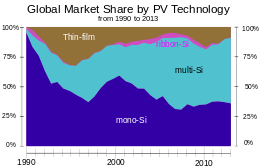
Global market-share in terms of annual production by PV technology since 1990

Solar cells are typically named after the semiconducting material they are made of. These materials must have certain characteristics in order to absorb sunlight. Some cells are designed to handle sunlight that reaches the Earth's surface, while others are optimized for use in space. Solar cells can be made of only one single layer of light-absorbing material (single-junction) or use multiple physical configurations (multi-junctions) to take advantage of various absorption and charge separation mechanisms.

Solar cells can be classified into first, second and third generation cells. The first generation cells—also called conventional, traditional or wafer-based cells—are made of crystalline silicon, the commercially predominant PV technology, that includes materials such as polysilicon and monocrystalline silicon. Second generation cells are thin film solar cells, that include amorphous silicon, CdTe and CIGS cells and are commercially significant in utility-scale photovoltaic power stations, building integrated photovoltaics or in small stand-alone power system. The third generation of solar cells includes a number of thin-film technologies often described as emerging photovoltaics—most of them have not yet been commercially applied and are still in the research or development phase. Many use organic materials, often organometallic compounds as well as inorganic substances. Despite the fact that their efficiencies had been low and the stability of the absorber material was often too short for commercial applications, there is a lot of research invested into these technologies as they promise to achieve the goal of producing low-cost, high-efficiency solar cells.

Crystalline silicon

By far, the most prevalent bulk material for solar cells is crystalline silicon (c-Si), also known as "solar grade silicon". Bulk silicon is separated into multiple categories according to crystallinity and crystal size in the resulting ingot, ribbon or wafer. These cells are entirely based around the concept of a p-n junction. Solar cells made of c-Si are made from wafers between 160 to 240 micrometers thick.

Monocrystalline silicon

Monocrystalline silicon (mono-Si) solar cells are more efficient and more expensive than most other types of cells. The corners of the cells look clipped, like an octagon, because the wafer material is cut from cylindrical ingots, that are typically grown by the Czochralski process. Solar panels using mono-Si cells display a distinctive pattern of small white diamonds.

Epitaxial silicon

Epitaxial wafers can be grown on a monocrystalline silicon "seed" wafer by atmospheric-pressure CVD in a high-throughput inline process, and then detached as self-supporting wafers of some standard thickness (e.g., 250 µm) that can be manipulated by hand, and directly substituted for wafer cells cut from monocrystalline silicon ingots. Solar cells made with this technique can have efficiencies approaching those of wafer-cut cells, but at appreciably lower cost.[36]

Polycrystalline silicon 

Polycrystalline silicon, or multicrystalline silicon (multi-Si) cells are made from cast square ingots—large blocks of molten silicon carefully cooled and solidified. They consist of small crystals giving the material its typical metal flake effect. Polysilicon cells are the most common type used in photovoltaics and are less expensive, but also less efficient, than those made from monocrystalline silicon.

Ribbon silicon 

Ribbon silicon is a type of polycrystalline silicon—it is formed by drawing flat thin films from molten silicon and results in a polycrystalline structure. These cells are cheaper to make than multi-Si, due to a great reduction in silicon waste, as this approach does not require sawing from ingots.[37] However, they are also less efficient.

Mono-like-multi silicon (MLM) 

This form was developed in the 2000s and introduced commercially around 2009. Also called cast-mono, this design uses polycrystalline casting chambers with small "seeds" of mono material. The result is a bulk mono-like material that is polycrystalline around the outsides. When sliced for processing, the inner sections are high-efficiency mono-like cells (but square instead of "clipped"), while the outer edges are sold as conventional poly. This production method results in mono-like cells at poly-like prices.[38]

Thin film

Thin-film technologies reduce the amount of active material in a cell. Most designs sandwich active material between two panes of glass. Since silicon solar panels only use one pane of glass, thin film panels are approximately twice as heavy as crystalline silicon panels, although they have a smaller ecological impact (determined from life cycle analysis).[39] The majority of film panels have 2-3 percentage points lower conversion efficiencies than crystalline silicon.[40] Cadmium telluride (CdTe), copper indium gallium selenide (CIGS) and amorphous silicon (a-Si) are three thin-film technologies often used for outdoor applications. As of December 2013, CdTe cost per installed watt was $0.59 as reported by First Solar. CIGS technology laboratory demonstrations reached 20.4% conversion efficiency as of December 2013. The lab efficiency of GaAs thin film technology topped 28%.[citation needed] The quantum efficiency of thin film solar cells is also lower due to reduced number of collected charge carriers per incident photon. Most recently, CZTS solar cell emerge as the less-toxic thin film solar cell technology, which achieved ~12% efficiency.[41] Thin film solar cells are increasing due to it being silent, renewable and solar energy being the most abundant energy source on Earth.[42]

Cadmium telluride

Cadmium telluride is the only thin film material so far to rival crystalline silicon in cost/watt. However cadmium is highly toxic and tellurium (anion: "telluride") supplies are limited. The cadmium present in the cells would be toxic if released. However, release is impossible during normal operation of the cells and is unlikely during fires in residential roofs.[43] A square meter of CdTe contains approximately the same amount of Cd as a single C cell nickel-cadmium battery, in a more stable and less soluble form.[43]

Copper indium gallium selenide

Copper indium gallium selenide (CIGS) is a direct band gap material. It has the highest efficiency (~20%) among all commercially significant thin film materials (see CIGS solar cell). Traditional methods of fabrication involve vacuum processes including co-evaporation and sputtering. Recent developments at IBM and Nanosolar attempt to lower the cost by using non-vacuum solution processes.[44]

Silicon thin film 

Silicon thin-film cells are mainly deposited by chemical vapor deposition (typically plasma-enhanced, PE-CVD) from silane gas and hydrogen gas. Depending on the deposition parameters, this can yield amorphous silicon (a-Si or a-Si:H), protocrystalline silicon or nanocrystalline silicon (nc-Si or nc-Si:H), also called microcrystalline silicon.[45]

Amorphous silicon is the most well-developed thin film technology to-date. An amorphous silicon (a-Si) solar cell is made of non-crystalline or microcrystalline silicon. Amorphous silicon has a higher bandgap (1.7 eV) than crystalline silicon (c-Si) (1.1 eV), which means it absorbs the visible part of the solar spectrum more strongly than the higher power density infrared portion of the spectrum. The production of a-Si thin film solar cells uses glass as a substrate and deposits a very thin layer of silicon by plasma-enhanced chemical vapor deposition (PECVD).

Protocrystalline silicon with a low volume fraction of nanocrystalline silicon is optimal for high open circuit voltage.[46] Nc-Si has about the same bandgap as c-Si and nc-Si and a-Si can advantageously be combined in thin layers, creating a layered cell called a tandem cell. The top cell in a-Si absorbs the visible light and leaves the infrared part of the spectrum for the bottom cell in nc-Si.

Gallium arsenide thin filmT

The semiconductor material Gallium arsenide (GaAs) is also used for single-crystalline thin film solar cells. Although GaAs cells are very expensive, they hold the world's record in efficiency for a single-junction solar cell at 28.8%.[47] GaAs is more commonly used in multijunction photovoltaic cells for concentrated photovoltaics (CPV, HCPV) and for solar panels on spacecrafts, as the industry favours efficiency over cost for space-based solar power.

Multijunction cells


Dawn's 10 kW triple-junction gallium arsenide solar array at full extension

Multi-junction cells consist of multiple thin films, each essentially a solar cell grown on top of each other, typically using metalorganic vapour phase epitaxy. Each layers has a different band gap energy to allow it to absorb electromagnetic radiation over a different portion of the spectrum. Multi-junction cells were originally developed for special applications such as satellites and space exploration, but are now used increasingly in terrestrial concentrator photovoltaics (CPV), an emerging technology that uses lenses and curved mirrors to concentrate sunlight onto small but highly efficient multi-junction solar cells. By concentrating sunlight up to a thousand times, High concentrated photovoltaics (HCPV) has the potential to outcompete conventional solar PV in the future.[48]:21,26
Tandem solar cells based on monolithic, series connected, gallium indium phosphide (GaInP), gallium arsenide (GaAs), and germanium (Ge) p–n junctions, are increasing sales, despite cost pressures.[49] Between December 2006 and December 2007, the cost of 4N gallium metal rose from about $350 per kg to $680 per kg. Additionally, germanium metal prices have risen substantially to $1000–1200 per kg this year. Those materials include gallium (4N, 6N and 7N Ga), arsenic (4N, 6N and 7N) and germanium, pyrolitic boron nitride (pBN) crucibles for growing crystals, and boron oxide, these products are critical to the entire substrate manufacturing industry.[citation needed]
A triple-junction cell, for example, may consist of the semiconductors: GaAs, Ge, and GaInP
2
.[50] Triple-junction GaAs solar cells were used as the power source of the Dutch four-time World Solar Challenge winners Nuna in 2003, 2005 and 2007 and by the Dutch solar cars Solutra (2005), Twente One (2007) and 21Revolution (2009).[citation needed] GaAs based multi-junction devices are the most efficient solar cells to date. On 15 October 2012, triple junction metamorphic cells reached a record high of 44%.[51]

Research in solar cells

Perovskite solar cells

Perovskite solar cells are solar cells that include a perovskite-structured material as the active layer. Most commonly, this is a solution-processed hybrid organic-inorganic tin or lead halide based material. Efficiencies have increased from below 10% at their first usage in 2009 to over 20% in 2014, making them a very rapidly advancing technology and a hot topic in the solar cell field.[52] Perovskite solar cells are also forecast to be extremely cheap to scale up, making them a very attractive option for commercialisation.

Liquid inks

In 2014, researchers at California NanoSystems Institute discovered using kesterite and perovskite improved electric power conversion efficiency for solar cells.[53]

Upconversion and Downconversion

Photon upconversion is the process of using two low-energy (e.g., infrared) photons to produce one higher energy photon; downconversion is the process of using one high energy photon (e.g.,, ultraviolet) to produce two lower energy photons. Either of these techniques could be used to produce higher efficiency solar cells by allowing solar photons to be more efficiently used. The difficulty, however, is that the conversion efficiency of existing phosphors exhibiting up- or down-conversion is low, and is typically narrow band.

One upconversion technique is to incorporate lanthanide-doped materials (Er3+, Yb3+, Ho3+ or a combination), taking advantage of their luminescence to convert infrared radiation to visible light. Upconversion process occurs when two infrared photons are absorbed by rare-earth ions to generate a (high-energy) absorbable photon. As example, the energy transfer upconversion process (ETU), consists in successive transfer processes between excited ions in the near infrared. The upconverter material could be placed below the solar cell to absorb the infrared light that passes through the silicon. Useful ions are most commonly found in the trivalent state. Er+ ions have been the most used. Er3+ ions absorb solar radiation around 1.54 µm. Two Er3+ ions that have absorbed this radiation can interact with each other through an upconversion process. The excited ion emits light above the Si bandgap that is absorbed by the solar cell and creates an additional electron–hole pair that can generate current. However, the increased efficiency was small. In addition, fluoroindate glasses have low phonon energy and have been proposed as suitable matrix doped with Ho3+ ions.[54]

Light-absorbing dyes

Dye-sensitized solar cells (DSSCs) are made of low-cost materials and do not need elaborate manufacturing equipment, so they can be made in a DIY fashion. In bulk it should be significantly less expensive than older solid-state cell designs. DSSC's can be engineered into flexible sheets and although its conversion efficiency is less than the best thin film cells, its price/performance ratio may be high enough to allow them to compete with fossil fuel electrical generation.

Typically a ruthenium metalorganic dye (Ru-centered) is used as a monolayer of light-absorbing material. The dye-sensitized solar cell depends on a mesoporous layer of nanoparticulate titanium dioxide to greatly amplify the surface area (200–300 m2/g TiO
2
, as compared to approximately 10 m2/g of flat single crystal). The photogenerated electrons from the light absorbing dye are passed on to the n-type TiO
2
and the holes are absorbed by an electrolyte on the other side of the dye. The circuit is completed by a redox couple in the electrolyte, which can be liquid or solid. This type of cell allows more flexible use of materials and is typically manufactured by screen printing or ultrasonic nozzles, with the potential for lower processing costs than those used for bulk solar cells. However, the dyes in these cells also suffer from degradation under heat and UV light and the cell casing is difficult to seal due to the solvents used in assembly. The first commercial shipment of DSSC solar modules occurred in July 2009 from G24i Innovations.[55]

Quantum dots

Quantum dot solar cells (QDSCs) are based on the Gratzel cell, or dye-sensitized solar cell architecture, but employ low band gap semiconductor nanoparticles, fabricated with crystallite sizes small enough to form quantum dots (such as CdS, CdSe, Sb
2
S
3
, PbS, etc.), instead of organic or organometallic dyes as light absorbers. QD's size quantization allows for the band gap to be tuned by simply changing particle size. They also have high extinction coefficients and have shown the possibility of multiple exciton generation.[56]

In a QDSC, a mesoporous layer of titanium dioxide nanoparticles forms the backbone of the cell, much like in a DSSC. This TiO
2
layer can then be made photoactive by coating with semiconductor quantum dots using chemical bath deposition, electrophoretic deposition or successive ionic layer adsorption and reaction. The electrical circuit is then completed through the use of a liquid or solid redox couple. The efficiency of QDSCs has increased[57] to over 5% shown for both liquid-junction[58] and solid state cells.[59] In an effort to decrease production costs, the Prashant Kamat research group[60] demonstrated a solar paint made with TiO
2
and CdSe that can be applied using a one-step method to any conductive surface with efficiencies over 1%.[61]

Organic/polymer solar cells

Organic solar cells and polymer solar cells are built from thin films (typically 100 nm) of organic semiconductors including polymers, such as polyphenylene vinylene and small-molecule compounds like copper phthalocyanine (a blue or green organic pigment) and carbon fullerenes and fullerene derivatives such as PCBM.

They can be processed from liquid solution, offering the possibility of a simple roll-to-roll printing process, potentially leading to inexpensive, large-scale production. In addition, these cells could be beneficial for some applications where mechanical flexibility and disposability are important. Current cell efficiencies are, however, very low, and practical devices are essentially non-existent.
Energy conversion efficiencies achieved to date using conductive polymers are very low compared to inorganic materials. However, Konarka Power Plastic reached efficiency of 8.3%[62] and organic tandem cells in 2012 reached 11.1%.[citation needed]

The active region of an organic device consists of two materials, one electron donor and one electron acceptor. When a photon is converted into an electron hole pair, typically in the donor material, the charges tend to remain bound in the form of an exciton, separating when the exciton diffuses to the donor-acceptor interface, unlike most other solar cell types. The short exciton diffusion lengths of most polymer systems tend to limit the efficiency of such devices. Nanostructured interfaces, sometimes in the form of bulk heterojunctions, can improve performance.[63]

In 2011, MIT and Michigan State researchers developed solar cells with a power efficiency close to 2% with a transparency to the human eye greater than 65%, achieved by selectively absorbing the ultraviolet and near-infrared parts of the spectrum with small-molecule compounds.[64][65] Researchers at UCLA more recently developed an analogous polymer solar cell, following the same approach, that is 70% transparent and has a 4% power conversion efficiency.[66][67][68] These lightweight, flexible cells can be produced in bulk at a low cost and could be used to create power generating windows.

In 2013, researchers announced polymer cells with some 3% efficiency. They used block copolymers, self-assembling organic materials that arrange themselves into distinct layers. The research focused on P3HT-b-PFTBT that separates into bands some 16 nanometers wide.[69][70]

Adaptive cells

Adaptive cells change their absorption/reflection characteristics depending to respond to environmental conditions. An adaptive material responds to the intensity and angle of incident light. At the part of the cell where the light is most intense, the cell surface changes from reflective to adaptive, allowing the light to penetrate the cell. The other parts of the cell remain reflective increasing the retention of the absorbed light within the cell.[71]

In 2014 a system that combined an adaptive surface with a glass substrate that redirect the absorbed to a light absorber on the edges of the sheet. The system also included an array of fixed lenses/mirrors to concentrate light onto the adaptive surface. As the day continues, the concentrated light moves along the surface of the cell. That surface switches from reflective to adaptive when the light is most concentrated and back to reflective after the light moves along.[71]

Manufacture


Solar cells share some of the same processing and manufacturing techniques as other semiconductor devices. However, the stringent requirements for cleanliness and quality control of semiconductor fabrication are more relaxed for solar cells, lowering costs.

Polycrystalline silicon wafers are made by wire-sawing block-cast silicon ingots into 180 to 350 micrometer wafers. The wafers are usually lightly p-type-doped. A surface diffusion of n-type dopants is performed on the front side of the wafer. This forms a p–n junction a few hundred nanometers below the surface.

Anti-reflection coatings are then typically applied to increase the amount of light coupled into the solar cell. Silicon nitride has gradually replaced titanium dioxide as the preferred material, because of its excellent surface passivation qualities. It prevents carrier recombination at the cell surface. A layer several hundred nanometers thick is applied using PECVD. Some solar cells have textured front surfaces that, like anti-reflection coatings, increase the amount of light reaching the wafer. Such surfaces were first applied to single-crystal silicon, followed by multicrystalline silicon somewhat later.

A full area metal contact is made on the back surface, and a grid-like metal contact made up of fine "fingers" and larger "bus bars" are screen-printed onto the front surface using a silver paste. This is an evolution of the so-called "wet" process for applying electrodes, first described in a US patent filed in 1981 by Bayer AG.[72] The rear contact is formed by screen-printing a metal paste, typically aluminium. Usually this contact covers the entire rear, though some designs employ a grid pattern. The paste is then fired at several hundred degrees Celsius to form metal electrodes in ohmic contact with the silicon. Some companies use an additional electro-plating step to increase efficiency. After the metal contacts are made, the solar cells are interconnected by flat wires or metal ribbons, and assembled into modules or "solar panels". Solar panels have a sheet of tempered glass on the front, and a polymer encapsulation on the back.

Manufacturers and certification

Solar cell production by region[73]

National Renewable Energy Laboratory tests and validates solar technologies. Three reliable groups certify solar equipment: UL and IEEE (both U.S. standards) and IEC.

Solar cells are manufactured in volume in Japan, Germany, China, Taiwan, Malaysia and the United States, whereas Europe, China, the U.S., and Japan have dominated (94% or more as of 2013) in installed systems.[74] Other nations are acquiring significant solar cell production capacity.

Global PV cell/module production increased by 10% in 2012 despite a 9% decline in solar energy investments according to the annual "PV Status Report" released by the European Commission's Joint Research Centre. Between 2009 and 2013 cell production has quadrupled.[74][75][76]

China

Due to heavy government investment, China has become the dominant force in solar cell manufacturing. Chinese companies produced solar cells/modules with a capacity of ~23 GW in 2013 (60% of global production).[74]

Malaysia

In 2014, Malaysia was the world's third largest manufacturer of photovoltaics equipment, behind China and the European Union.[77]

United States

Solar cell production in the U.S. has suffered due to the global financial crisis, but recovered partly due to the falling price of quality silicon.[78][79]

Volcanism on Io

From Wikipedia, the free encyclopedia https://en.wikipedia.org/wiki/Volcanism_on_Io   Io, with two plumes...