Coriolis force

From Wikipedia, the free encyclopedia

 .

In the inertial frame of reference (upper part of the picture), the black ball moves in a straight line. However, the observer (red dot) who is standing in the rotating/non-inertial frame of reference (lower part of the picture) sees the object as following a curved path due to the Coriolis and centrifugal forces present in this frame.

In physics, the Coriolis force is an inertial force (also called a fictitious force) acting on objects which are in motion relative to a rotating reference frame. In a reference frame with clockwise rotation, the force acts to the left of the motion of the object; in one with anticlockwise rotation, the force acts to the right. Although recognized previously by others, the mathematical expression for the Coriolis force appeared in an 1835 paper by French scientist Gaspard-Gustave de Coriolis, in connection with the theory of water wheels. Early in the 20th century, the term Coriolis force began to be used in connection with meteorology. Deflection of an object due to the Coriolis force is called the 'Coriolis effect'.

Newton's laws of motion describe the motion of an object in an inertial (non-accelerating) frame of reference. When Newton's laws are transformed to a rotating frame of reference, the Coriolis force and centrifugal force appear. Both forces are proportional to the mass of the object. The Coriolis force is proportional to the rotation rate and the centrifugal force is proportional to its square. The Coriolis force acts in a direction perpendicular to the rotation axis and to the velocity of the body in the rotating frame and is proportional to the object's speed in the rotating frame. The centrifugal force acts outwards in the radial direction and is proportional to the distance of the body from the axis of the rotating frame. These additional forces are termed inertial forces, fictitious forces or pseudo forces.^[1] They allow the application of Newton's laws to a rotating system. They are correction factors that do not exist in a non-accelerating or inertial reference frame.

A commonly encountered rotating reference frame is the Earth. The Coriolis effect is caused by the rotation of the Earth and the inertia of the mass experiencing the effect. Because the Earth completes only one rotation per day, the Coriolis force is quite small, and its effects generally become noticeable only for motions occurring over large distances and long periods of time, such as large-scale movement of air in the atmosphere or water in the ocean. Such motions are constrained by the surface of the Earth, so only the horizontal component of the Coriolis force is generally important. This force causes moving objects on the surface of the Earth to be deflected to the right (with respect to the direction of travel) in the Northern Hemisphere and to the left in the Southern Hemisphere. The horizontal deflection effect is greater near the poles and smallest at the equator, since the rate of change in the diameter of the circles of latitude when travelling north or south, increases the closer the object is to the poles.^[2] Rather than flowing directly from areas of high pressure to low pressure, as they would in a non-rotating system, winds and currents tend to flow to the right of this direction north of the equator and to the left of this direction south of it. This effect is responsible for the rotation of large cyclones (see Coriolis effects in meteorology). To explain this intuitively, consider how an object that moves northwards from the equator has a tendency to maintain its greater speed at the equator (rotating around towards the right as you look at the sphere of the Earth), where the "horizontal diameter" is larger, and therefore tends to move towards the right as it passed northwards where the "horizontal diameter" of the Earth (the rings of latitude) is smaller, and the linear speed of local objects on the Earth's surface at that latitude is slower.

History

Italian scientists Giovanni Battista Riccioli and his assistant Francesco Maria Grimaldi described the effect in connection with artillery in the 1651 Almagestum Novum, writing that rotation of the Earth should cause a cannonball fired to the north to deflect to the east.^[3] The effect was described in the tidal equations of Pierre-Simon Laplace in 1778.

Gaspard-Gustave Coriolis published a paper in 1835 on the energy yield of machines with rotating parts, such as waterwheels.^[4] That paper considered the supplementary forces that are detected in a rotating frame of reference. Coriolis divided these supplementary forces into two categories. The second category contained a force that arises from the cross product of the angular velocity of a coordinate system and the projection of a particle's velocity into a plane perpendicular to the system's axis of rotation. Coriolis referred to this force as the "compound centrifugal force" due to its analogies with the centrifugal force already considered in category one.^[5][6] The effect was known in the early 20th century as the "acceleration of Coriolis",^[7] and by 1920 as "Coriolis force".^[8]
In 1856, William Ferrel proposed the existence of a circulation cell in the mid-latitudes with air being deflected by the Coriolis force to create the prevailing westerly winds.^[9]

Understanding the kinematics of how exactly the rotation of the Earth affects airflow was partial at first.^[10] Late in the 19th century, the full extent of the large scale interaction of pressure gradient force and deflecting force that in the end causes air masses to move 'along' isobars was understood.^{[citation needed]}

Formula

In non-vector terms: at a given rate of rotation of the observer, the magnitude of the Coriolis acceleration of the object is proportional to the velocity of the object and also to the sine of the angle between the direction of movement of the object and the axis of rotation.

The vector formula for the magnitude and direction of the Coriolis acceleration ^[11] is

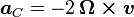
where (here and below) is the acceleration of the particle in the rotating system, is the velocity of the particle with respect to the rotating system, and Ω is the angular velocity vector which has magnitude equal to the rotation rate ω and is directed along the axis of rotation of the rotating reference frame, and the × symbol represents the cross product operator.

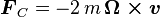
The equation may be multiplied by the mass of the relevant object to produce the Coriolis force:

.

The Coriolis effect is the behavior added by the Coriolis acceleration. The formula implies that the Coriolis acceleration is perpendicular both to the direction of the velocity of the moving mass and to the frame's rotation axis. So in particular:

• if the velocity is parallel to the rotation axis, the Coriolis acceleration is zero.
• if the velocity is straight inward to the axis, the acceleration is in the direction of local rotation.
• if the velocity is straight outward from the axis, the acceleration is against the direction of local rotation.
• if the velocity is in the direction of local rotation, the acceleration is outward from the axis.
• if the velocity is against the direction of local rotation, the acceleration is inward to the axis.

The vector cross product can be evaluated as the determinant of a matrix:

where the vectors i, j, k are unit vectors in the x, y and z directions.

Causes

The Coriolis force exists only when one uses a rotating reference frame. In the rotating frame it behaves exactly like a real force (that is to say, it causes acceleration and has real effects). However, the Coriolis force is a consequence of inertia,^[12] and is not attributable to an identifiable originating body, as is the case for electromagnetic or nuclear forces, for example. From an analytical viewpoint, to use Newton's second law in a rotating system, the Coriolis force is mathematically necessary, but it disappears in a non-accelerating, inertial frame of reference. For example, consider two children on opposite sides of a spinning roundabout (Merry-go-round ), who are throwing a ball to each other.
From the children's point of view, this ball's path is curved sideways by the Coriolis force. Suppose the roundabout spins anticlockwise when viewed from above. From the thrower's perspective, the deflection is to the right.^[13] From the non-thrower's perspective, deflection is to left. For a mathematical formulation see Mathematical derivation of fictitious forces.

An observer in a rotating frame, such as an astronaut in a rotating space station, very probably will find the interpretation of everyday life in terms of the Coriolis force accords more simply with intuition and experience than a cerebral reinterpretation of events from an inertial standpoint. For example, nausea due to an experienced push^{[clarification needed]} may be more instinctively explained by the Coriolis force than by the law of inertia.^[14][15] See also Coriolis effect (perception). In meteorology, a rotating frame (the Earth) with its Coriolis force provides a more natural framework for explanation of air movements than a non-rotating, inertial frame without Coriolis forces.^[16] In long-range gunnery, sight corrections for the Earth's rotation are based upon the Coriolis force.^[17] These examples are described in more detail below.

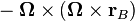
The acceleration entering the Coriolis force arises from two sources of change in velocity that result from rotation: the first is the change of the velocity of an object in time. The same velocity (in an inertial frame of reference where the normal laws of physics apply) will be seen as different velocities at different times in a rotating frame of reference. The apparent acceleration is proportional to the angular velocity of the reference frame (the rate at which the coordinate axes change direction), and to the component of velocity of the object in a plane perpendicular to the axis of rotation. This gives a term . The minus sign arises from the traditional definition of the cross product (right hand rule), and from the sign convention for angular velocity vectors.

The second is the change of velocity in space. Different positions in a rotating frame of reference have different velocities (as seen from an inertial frame of reference). In order for an object to move in a straight line it must therefore be accelerated so that its velocity changes from point to point by the same amount as the velocities of the frame of reference. The force is proportional to the angular velocity (which determines the relative speed of two different points in the rotating frame of reference), and to the component of the velocity of the object in a plane perpendicular to the axis of rotation (which determines how quickly it moves between those points). This also gives a term .

Length scales and the Rossby number

The time, space and velocity scales are important in determining the importance of the Coriolis force. Whether rotation is important in a system can be determined by its Rossby number, which is the ratio of the velocity, U, of a system to the product of the Coriolis parameter,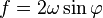, and the length scale, L, of the motion:

The Rossby number is the ratio of inertial to Coriolis forces. A small Rossby number signifies a system which is strongly affected by Coriolis forces, and a large Rossby number signifies a system in which inertial forces dominate. For example, in tornadoes, the Rossby number is large, in low-pressure systems it is low and in oceanic systems it is around 1. As a result, in tornadoes the Coriolis force is negligible, and balance is between pressure and centrifugal forces. In low-pressure systems, centrifugal force is negligible and balance is between Coriolis and pressure forces. In the oceans all three forces are comparable.^[18]

An atmospheric system moving at U = 10 m/s (22 mph) occupying a spatial distance of L = 1,000 km (621 mi), has a Rossby number of approximately 0.1.

A baseball pitcher may throw the ball at U = 45 m/s (100 mph) for a distance of L = 18.3 m (60 ft). The Rossby number in this case would be 32,000.

Needless to say, one does not worry about which hemisphere one is in when playing baseball. However, an unguided missile obeys exactly the same physics as a baseball, but may travel far enough and be in the air long enough to notice the effect of Coriolis force. Long-range shells in the Northern Hemisphere landed close to, but to the right of, where they were aimed until this was noted. (Those fired in the Southern Hemisphere landed to the left.) In fact, it was this effect that first got the attention of Coriolis himself.^[19][20][21]

Simple cases

Cannon on turntable

Cannon at the center of a rotating turntable. To hit the target located at position 1 on the perimeter at time t = 0 s, the cannon must be aimed ahead of the target at angle θ. That way, by the time the cannonball reaches position 3 on the periphery, the target also will be at that position. In an inertial frame of reference, the cannonball travels a straight radial path to the target (curve y_A). However, in the frame of the turntable, the path is arched (curve y_B), as also shown in the figure.

Successful trajectory of cannonball as seen from the turntable for three angles of launch θ. Plotted points are for the same equally spaced times steps on each curve. Cannonball speed v is held constant and angular rate of rotation ω is varied to achieve a successful "hit" for selected θ. For example, for a radius of 1 m and a cannonball speed of 1 m/s, the time of flight t_f = 1 s, and ωt_f = θ → ω and θ have the same numerical value if θ is expressed in radians. The wider spacing of the plotted points as the target is approached show the speed of the cannonball is accelerating as seen on the turntable, due to fictitious Coriolis and centrifugal forces.

Acceleration components at an earlier time (top) and at arrival time at the target (bottom)

Coriolis acceleration, centrifugal acceleration and net acceleration vectors at three selected points on the trajectory as seen on the turntable.

The animation at the top of this article is a classic illustration of Coriolis force. Another visualization of the Coriolis and centrifugal forces is this animation clip.
Given the radius R of the turntable in that animation, the rate of angular rotation ω, and the speed of the cannonball (assumed constant) v, the correct angle θ to aim so as to hit the target at the edge of the turntable can be calculated.

The inertial frame of reference provides one way to handle the question: calculate the time to interception, which is t_f = R / v . Then, the turntable revolves an angle ω t_f in this time. If the cannon is pointed an angle θ = ω t_f = ω R / v, then the cannonball arrives at the periphery at position number 3 at the same time as the target.

No discussion of Coriolis force can arrive at this solution as simply, so the reason to treat this problem is to demonstrate Coriolis formalism in an easily visualized situation.

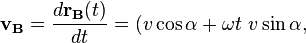
Trajectory in the Inertial Frame

The trajectory in the inertial frame (denoted A) is a straight line radial path at angle θ. The position of the cannonball in (x, y) coordinates at time t is:

In the turntable frame (denoted B), the x- y axes rotate at angular rate ω, so the trajectory becomes:

and three examples of this result are plotted in the figure.

Accelerations

Components of Acceleration

To determine the components of acceleration, a general expression is used from the article fictitious force:

   

in which the term in Ω × v_B is the Coriolis acceleration and the term in Ω × ( Ω × r_B) is the centrifugal acceleration. The results are (let α = θ − ωt):

  

 

Producing Accelerations

Producing a centrifugal acceleration:

 

Also:

 

  

producing a Coriolis acceleration:

 

 

These accelerations are shown in the diagrams for a particular example.

It is seen that the Coriolis acceleration not only cancels the centrifugal acceleration, but together they provide a net "centripetal", radially inward component of acceleration (that is, directed toward the center of rotation):^[22]

and an additional component of acceleration perpendicular to r_B (t):

 

The "centripetal" component of acceleration resembles that for circular motion at radius r_B, while the perpendicular component is velocity dependent, increasing with the radial velocity v and directed to the right of the velocity. The situation could be described as a circular motion combined with an "apparent Coriolis acceleration" of 2ωv. However, this is a rough labelling: a careful designation of the true centripetal force refers to a local reference frame that employs the directions normal and tangential to the path, not coordinates referred to the axis of rotation.

These results also can be obtained directly by two time differentiations of r_B (t). Agreement of the two approaches demonstrates that one could start from the general expression for fictitious acceleration above and derive the trajectories shown here. However, working from the acceleration to the trajectory is more complicated than the reverse procedure used here, which, of course, is made possible in this example by knowing the answer in advance.

As a result of this analysis an important point appears: all the fictitious accelerations must be included to obtain the correct trajectory. In particular, besides the Coriolis acceleration, the centrifugal force plays an essential role. It is easy to get the impression from verbal discussions of the cannonball problem, which are focussed on displaying the Coriolis effect particularly, that the Coriolis force is the only factor that must be considered;^[23] emphatically, that is not so.^[24] A turntable for which the Coriolis force is the only factor is the parabolic turntable. A somewhat more complex situation is the idealized example of flight routes over long distances, where the centrifugal force of the path and aeronautical lift are countered by gravitational attraction.^[25][26]

Tossed ball on a rotating carousel

A carousel is rotating counter-clockwise. Left panel: a ball is tossed by a thrower at 12:00 o'clock and travels in a straight line to the center of the carousel. While it travels, the thrower circles in a counter-clockwise direction. Right panel: The ball's motion as seen by the thrower, who now remains at 12:00 o'clock, because there is no rotation from their viewpoint.

The figure illustrates a ball tossed from 12:00 o'clock toward the center of a counter-clockwise rotating carousel. On the left, the ball is seen by a stationary observer above the carousel, and the ball travels in a straight line to the center, while the ball-thrower rotates counter-clockwise with the carousel. On the right the ball is seen by an observer rotating with the carousel, so the ball-thrower appears to stay at 12:00 o'clock. The figure shows how the trajectory of the ball as seen by the rotating observer can be constructed.
On the left, two arrows locate the ball relative to the ball-thrower. One of these arrows is from the thrower to the center of the carousel (providing the ball-thrower's line of sight), and the other points from the center of the carousel to the ball.(This arrow gets shorter as the ball approaches the center.) A shifted version of the two arrows is shown dotted.

On the right is shown this same dotted pair of arrows, but now the pair are rigidly rotated so the arrow corresponding to the line of sight of the ball-thrower toward the center of the carousel is aligned with 12:00 o'clock. The other arrow of the pair locates the ball relative to the center of the carousel, providing the position of the ball as seen by the rotating observer. By following this procedure for several positions, the trajectory in the rotating frame of reference is established as shown by the curved path in the right-hand panel.

The ball travels in the air, and there is no net force upon it. To the stationary observer the ball follows a straight-line path, so there is no problem squaring this trajectory with zero net force. However, the rotating observer sees a curved path. Kinematics insists that a force (pushing to the right of the instantaneous direction of travel for a counter-clockwise rotation) must be present to cause this curvature, so the rotating observer is forced to invoke a combination of centrifugal and Coriolis forces to provide the net force required to cause the curved trajectory.

Bounced ball

Bird's-eye view of carousel. The carousel rotates clockwise. Two viewpoints are illustrated: that of the camera at the center of rotation rotating with the carousel (left panel) and that of the inertial (stationary) observer (right panel). Both observers agree at any given time just how far the ball is from the center of the carousel, but not on its orientation. Time intervals are 1/10 of time from launch to bounce.

The figure describes a more complex situation where the tossed ball on a turntable bounces off the edge of the carousel and then returns to the tosser, who catches the ball. The effect of Coriolis force on its trajectory is shown again as seen by two observers: an observer (referred to as the "camera") that rotates with the carousel, and an inertial observer. The figure shows a bird's-eye view based upon the same ball speed on forward and return paths. Within each circle, plotted dots show the same time points. In the left panel, from the camera's viewpoint at the center of rotation, the tosser (smiley face) and the rail both are at fixed locations, and the ball makes a very considerable arc on its travel toward the rail, and takes a more direct route on the way back. From the ball tosser's viewpoint, the ball seems to return more quickly than it went (because the tosser is rotating toward the ball on the return flight).

On the carousel, instead of tossing the ball straight at a rail to bounce back, the tosser must throw the ball toward the right of the target and the ball then seems to the camera to bear continuously to the left of its direction of travel to hit the rail (left because the carousel is turning clockwise). The ball appears to bear to the left from direction of travel on both inward and return trajectories. The curved path demands this observer to recognize a leftward net force on the ball. (This force is "fictitious" because it disappears for a stationary observer, as is discussed shortly.) For some angles of launch, a path has portions where the trajectory is approximately radial, and Coriolis force is primarily responsible for the apparent deflection of the ball (centrifugal force is radial from the center of rotation, and causes little deflection on these segments). When a path curves away from radial, however, centrifugal force contributes significantly to deflection.

The ball's path through the air is straight when viewed by observers standing on the ground (right panel). In the right panel (stationary observer), the ball tosser (smiley face) is at 12 o'clock and the rail the ball bounces from is at position one (1). From the inertial viewer's standpoint, positions one (1), two (2), three (3) are occupied in sequence. At position 2 the ball strikes the rail, and at position 3 the ball returns to the tosser. Straight-line paths are followed because the ball is in free flight, so this observer requires that no net force is applied.

Applied to the Earth

An important case where the Coriolis force is observed is the rotating Earth. Unless otherwise stated, directions of forces and motion apply to the Northern Hemisphere.

Intuitive explanation

As the Earth turns around its axis, everything attached to it turns with it (imperceptibly to our senses). An object that is moving without being dragged along with this rotation travels in a straight motion over the turning Earth. From our rotating perspective on the planet, its direction of motion changes as it moves, bending in the opposite direction to our actual motion. When viewed from a stationary point in space above, any land feature in the Northern Hemisphere turns anticlockwise, and, fixing our gaze on that location, any other location in that hemisphere will rotate around it the same way. The traced ground path of a freely moving body travelling from one point to another will therefore bend the opposite way, clockwise, which is conventionally labeled as "right," where it will be if the direction of motion is considered "ahead" and "down" is defined naturally.

Rotating sphere

Coordinate system at latitude φ with x-axis east, y-axis north and z-axis upward (that is, radially outward from center of sphere).

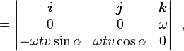
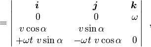
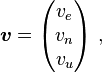
Consider a location with latitude φ on a sphere that is rotating around the north-south axis.^[27] A local coordinate system is set up with the x axis horizontally due east, the y axis horizontally due north and the z axis vertically upwards. The rotation vector, velocity of movement and Coriolis acceleration expressed in this local coordinate system (listing components in the order east (e), north (n) and upward (u)) are:

   

When considering atmospheric or oceanic dynamics, the vertical velocity is small, and the vertical component of the Coriolis acceleration is small compared to gravity. For such cases, only the horizontal (east and north) components matter. The restriction of the above to the horizontal plane is (setting v_u = 0):

   

where is called the Coriolis parameter.

By setting v_n = 0, it can be seen immediately that (for positive φ and ω) a movement due east results in an acceleration due south. Similarly, setting v_e = 0, it is seen that a movement due north results in an acceleration due east. In general, observed horizontally, looking along the direction of the movement causing the acceleration, the acceleration always is turned 90° to the right and of the same size regardless of the horizontal orientation.

As a different case, consider equatorial motion setting φ = 0°. In this case, Ω is parallel to the north or n-axis, and:

      

Accordingly, an eastward motion (that is, in the same direction as the rotation of the sphere) provides an upward acceleration known as the Eötvös effect, and an upward motion produces an acceleration due west.

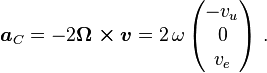
For additional examples in this article see cannon on turntable and tossed ball. In other articles, see rotating spheres, apparent motion of stationary objects, and carousel.

Meteorology

This low-pressure system over Iceland spins anticlockwise due to balance between the Coriolis force and the pressure gradient force.

Schematic representation of flow around a low-pressure area in the Northern Hemisphere. The Rossby number is low, so the centrifugal force is virtually negligible. The pressure-gradient force is represented by blue arrows, the Coriolis acceleration (always perpendicular to the velocity) by red arrows

Schematic representation of inertial circles of air masses in the absence of other forces, calculated for a wind speed of approximately 50 to 70 m/s (110 to 160 mph).

Cloud formations in a famous image of Earth from Apollo 17, makes similar circulation directly visible

Perhaps the most important impact of the Coriolis effect is in the large-scale dynamics of the oceans and the atmosphere. In meteorology and oceanography, it is convenient to postulate a rotating frame of reference wherein the Earth is stationary. In accommodation of that provisional postulation, the centrifugal and Coriolis forces are introduced. Their relative importance is determined by the applicable Rossby numbers. Tornadoes have high Rossby numbers, so, while tornado-associated centrifugal forces are quite substantial, Coriolis forces associated with tornadoes are for practical purposes negligible.^[28]

Because ocean currents are driven by the movement of wind over the water's surface, the Coriolis force also affects the movement of ocean currents and cyclones as well. Many of the ocean's largest currents circulate around warm, high-pressure areas called gyres. Though the circulation is not as significant as that in the air, the deflection caused by the Coriolis effect is what creates the spiraling pattern in these gyres. The spiraling wind pattern helps the hurricane form. The stronger the force from the Coriolis effect, the faster the wind will spin and pick up additional energy, increasing the strength of the hurricane.^[29]

Air within high-pressure systems rotates in a direction such that the Coriolis force will be directed radially inwards, and nearly balanced by the outwardly radial pressure gradient. As a result, air travels clockwise around high pressure in the Northern Hemisphere and anticlockwise in the Southern Hemisphere. Air within low-pressure systems rotates in the opposite direction, so that the Coriolis force is directed radially outward and nearly balances an inwardly radial pressure gradient.^{[citation needed]}

Flow around a low-pressure area

If a low-pressure area forms in the atmosphere, air will tend to flow in towards it, but will be deflected perpendicular to its velocity by the Coriolis force. A system of equilibrium can then establish itself creating circular movement, or a cyclonic flow. Because the Rossby number is low, the force balance is largely between the pressure gradient force acting towards the low-pressure area and the Coriolis force acting away from the center of the low pressure.
Instead of flowing down the gradient, large scale motions in the atmosphere and ocean tend to occur perpendicular to the pressure gradient. This is known as geostrophic flow.^[30] On a non-rotating planet, fluid would flow along the straightest possible line, quickly eliminating pressure gradients. Note that the geostrophic balance is thus very different from the case of "inertial motions" (see below) which explains why mid-latitude cyclones are larger by an order of magnitude than inertial circle flow would be.

This pattern of deflection, and the direction of movement, is called Buys-Ballot's law. In the atmosphere, the pattern of flow is called a cyclone. In the Northern Hemisphere the direction of movement around a low-pressure area is anticlockwise. In the Southern Hemisphere, the direction of movement is clockwise because the rotational dynamics is a mirror image there. At high altitudes, outward-spreading air rotates in the opposite direction.^[31] Cyclones rarely form along the equator due to the weak Coriolis effect present in this region.

Inertial circles

An air or water mass moving with speed subject only to the Coriolis force travels in a circular trajectory called an 'inertial circle'. Since the force is directed at right angles to the motion of the particle, it will move with a constant speed around a circle whose radius is given by:

where is the Coriolis parameter , introduced above (where is the latitude). The time taken for the mass to complete a full circle is therefore . The Coriolis parameter typically has a mid-latitude value of about 10⁻⁴ s⁻¹; hence for a typical atmospheric speed of 10 m/s (22 mph) the radius is 100 km (62 mi), with a period of about 17 hours. For an ocean current with a typical speed of 10 cm/s (0.22 mph), the radius of an inertial circle is 1 km (0.6 mi). These inertial circles are clockwise in the Northern Hemisphere (where trajectories are bent to the right) and anticlockwise in the Southern Hemisphere.

If the rotating system is a parabolic turntable, then is constant and the trajectories are exact circles. On a rotating planet, varies with latitude and the paths of particles do not form exact circles. Since the parameter varies as the sine of the latitude, the radius of the oscillations associated with a given speed are smallest at the poles (latitude = ±90°), and increase toward the equator.^[32]

Other terrestrial effects

The Coriolis effect strongly affects the large-scale oceanic and atmospheric circulation, leading to the formation of robust features like jet streams and western boundary currents. Such features are in geostrophic balance, meaning that the Coriolis and pressure gradient forces balance each other. Coriolis acceleration is also responsible for the propagation of many types of waves in the ocean and atmosphere, including Rossby waves and Kelvin waves. It is also instrumental in the so-called Ekman dynamics in the ocean, and in the establishment of the large-scale ocean flow pattern called the Sverdrup balance.

Eötvös effect

The practical impact of the "Coriolis effect" is mostly caused by the horizontal acceleration component produced by horizontal motion.
There are other components of the Coriolis effect. Westward-travelling objects will be deflected downwards (feel heavier), while Eastward-travelling objects will be deflected upwards (feel lighter).^[33] This is known as the Eötvös effect. This aspect of the Coriolis effect is greatest near the equator. The force produced by this effect is similar to the horizontal component, but the much larger vertical forces due to gravity and pressure mean that it is generally unimportant dynamically.
In addition, objects travelling upwards (i.e., out) or downwards (i.e., in) will be deflected to the west or east respectively. This effect is also the greatest near the equator. Since vertical movement is usually of limited extent and duration, the size of the effect is smaller and requires precise instruments to detect. However, in the case of large changes of momentum, such as a spacecraft being launched into orbit, the effect becomes significant. The fastest and most fuel-efficient path to orbit is a launch from the equator which curves to a directly eastward heading.

Intuitive example

One can imagine a train that travels through a frictionless railway line along the equator assuming that when it is in motion it does so at the necessary speed to complete a trip around the world in one day (465 m/s).^[34] The Coriolis effect can be considered in three cases: when the train travels west; when it is at rest and finally when it is travelling east. For each of this cases the Coriolis effect can be calculated from the rotating frame of reference on Earth first and then it can be checked against a fixed inertial frame. In the image below, the three cases are illustrated in an inertial frame as observed from a fixed point above Earth along its axis of rotation:

1. The train travels toward the west: In that case, it is moving against the direction of rotation. Therefore, on the Earth's rotating frame the Coriolis term will be pointed inwards towards the axis of rotation (down). This additional force downwards should cause the train to be heavier while moving in that direction.

• If one looks at this train from the fixed non-rotating frame on top of the center of the Earth, at that speed it remains stationary as the Earth spins beneath it. Hence, the only force acting on it would be gravity and the reaction from the track. This force is greater (by 0.34%)^[34] than the force that the passengers and the train experience when at rest (rotating along with Earth). This difference is what the Coriolis effect accounts for in the rotating frame of reference.

2. The train comes to a stop: From the point of view on the Earth's rotating frame, the velocity of the train is zero, thus the Coriolis force is also zero and the train and its passengers recuperate their usual weight.

• From the fixed inertial frame of reference above Earth, the train is now rotating along with the rest of the Earth. 0.34% of the force of gravity provides the centripetal force needed to achieve the circular motion on that frame of reference. The remaining force, as could be measured by a scale, would make the train and its passengers "lighter" than in the previous case.

3. The train changes direction and travels towards the East. In this case, as it is moving in the direction of Earth's rotating frame, the Coriolis term will be directed outward from the axis of rotation (up). This upward force would cause the train to seem lighter still than when at rest.

Graph of the force experienced by a 10 grams object as a function of its speed moving along Earth's equator (as measured within the rotating frame). (Positive force in the graph is directed upward. Positive speed is directed eastward and negative speed is directed westward).

• From the fixed frame of reference on space, the train travelling east will now be rotating at twice the rate as when it was at rest and therefore the amount of centripetal force needed to cause that circular path increases leaving less force from gravity to act on the track. This is what the Coriolis term accounts for on the previous paragraph.
• As a final check one can imagine a frame of reference rotating along with the train. Such frame would be rotating at twice the angular velocity as Earth's rotating frame. The resulting centrifugal force component for that imaginary frame would be greater. Since the train and its passengers are at rest, that would be the only component in that frame explaining again why the train and the passengers are lighter than in the previous two cases.

This also explains why high speed projectiles travelling west get deflected up and when travelling east are deflected down. This vertical component of the Coriolis effect is called the Eötvös effect.^[35]
The above example can be used to explain why the Eötvös effect starts diminishing on an object travelling westward as its tangential speed increases above Earth's rotation (465 m/s). If the westward train in the above example increases its speed, part of the force of gravity that was pushing against the track will account for the centripetal force needed to keep it in circular motion on the inertial frame. Once the train doubles its westward speed at 930 m/s that centripetal force will be equal to the force experienced by the train when it stops. From the inertial frame, in both cases it rotates at the same speed but in the opposite directions. Thus, the force is the same cancelling completely the Eötvös effect. Any object moving westward at a speed above 930 m/s would experience an upward force instead. In the figure, the Eötvös effect is illustrated for a 10 gram object on the train at different speeds. The parabolic shape is because the centripetal force is proportional to the square of the tangential speed. On the inertial frame, the bottom of the parabola would be centered at the origin. The offset is because, in this argument, the Earth's rotating frame of reference is being used. From the graph, it can be seen that the Eötvös effect is not symmetrical, and that the resulting downward force experienced by an object travelling west at high velocity is less than the resulting upward force when it is travelling east at the same speed.

Draining in bathtubs and toilets

Contrary to popular misconception, water rotation in home bathrooms under normal circumstances is not related to the Coriolis effect or to the rotation of the Earth, and no consistent difference in rotation direction between toilet drainage in the Northern and Southern Hemispheres can be observed. The formation of a vortex over the plug hole may be explained by the conservation of angular momentum: The radius of rotation decreases as water approaches the plug hole, so the rate of rotation increases, for the same reason that an ice skater's rate of spin increases as they pull their arms in. Any rotation around the plug hole that is initially present accelerates as water moves inward.

Of course, the Coriolis force does still impact the direction of the flow of water, but only minutely. Only if the water is so still that the effective rotation rate of the Earth is faster than that of the water relative to its container, and if externally applied torques (such as might be caused by flow over an uneven bottom surface) are small enough, the Coriolis effect may indeed determine the direction of the vortex. Without such careful preparation, the Coriolis effect will likely be much smaller than various other influences on drain direction^[36] such as any residual rotation of the water^[37] and the geometry of the container.^[38] Despite this, the idea that toilets and bathtubs drain differently in the Northern and Southern Hemispheres has been popularized by several television programs and films, including Escape Plan, Wedding Crashers, The Simpsons episode "Bart vs. Australia", and The X-Files episode "Die Hand Die Verletzt".^[39] Several science broadcasts and publications, including at least one college-level physics textbook, have also stated this.^[40][41]

In 1908, the Austrian physicist Ottokar Tumlirz described careful and effective experiments which demonstrated the effect of the rotation of the Earth on the outflow of water through a central aperture.^[42] The subject was later popularized in a famous 1962 article in the journal Nature, which described an experiment in which all other forces to the system were removed by filling a 6 ft (1.8 m) tank with 300 U.S. gal (1,100 L) of water and allowing it to settle for 24 hours (to allow any movement due to filling the tank to die away), in a room where the temperature had stabilized. The drain plug was then very slowly removed, and tiny pieces of floating wood were used to observe rotation. During the first 12 to 15 minutes, no rotation was observed. Then, a vortex appeared and consistently began to rotate in an anticlockwise direction (the experiment was performed in Boston, Massachusetts, in the Northern Hemisphere). This was repeated and the results averaged to make sure the effect was real. The report noted that the vortex rotated, "about 30,000 times faster than the effective rotation of the Earth in 42° North (the experiment's location)". This shows that the small initial rotation due to the Earth is amplified by gravitational draining and conservation of angular momentum to become a rapid vortex and may be observed under carefully controlled laboratory conditions.^[43][44]

Ballistic trajectories

The Coriolis force became important in external ballistics for calculating the trajectories of very long-range artillery shells. The most famous historical example was the Paris gun, used by the Germans during World War I to bombard Paris from a range of about 120 km (75 mi). Similarly, a bullet does not fly straight from the barrel to a target. The Coriolis force minutely changes the trajectory of a bullet, curving the path of the projectile into a more arched 'semi-circle' shape. This effect only affects accuracy at extremely long distances and is therefore adjusted for by accurate long-distance shooters, such as snipers and other trained professionals.^[17]

The effects of the Coriolis force on ballistic trajectories should not be confused with the curvature of the paths of missiles, satellites, and similar objects when the paths are plotted on two-dimensional (flat) maps, such as the Mercator projection. The projections of the three-dimensional curved surface of the Earth to a two-dimensional surface (the map) necessarily results in distorted features. The apparent curvature of the path is a consequence of the sphericity of the Earth and would occur even in a non-rotating frame.

Visualization of the Coriolis effect

Fluid assuming a parabolic shape as it is rotating

Object moving frictionlessly over the surface of a very shallow parabolic dish. The object has been released in such a way that it follows an elliptical trajectory.
Left: The inertial point of view.
Right: The co-rotating point of view.

The forces at play in the case of a curved surface.
Red: gravity
Green: the normal force
Blue: the net resultant centripetal force.

To demonstrate the Coriolis effect, a parabolic turntable can be used. On a flat turntable, the inertia of a co-rotating object would force it off the edge. But if the surface of the turntable has the correct paraboloid (parabolic bowl) shape (see the figure) and is rotated at the corresponding rate, the force components shown in the figure are such that the component of gravity tangential to the bowl surface will exactly equal the centripetal force necessary to keep the object rotating at its velocity and radius of curvature (assuming no friction). (See banked turn.) This carefully contoured surface allows the Coriolis force to be displayed in isolation.^[45][46]

Discs cut from cylinders of dry ice can be used as pucks, moving around almost frictionlessly over the surface of the parabolic turntable, allowing effects of Coriolis on dynamic phenomena to show themselves. To get a view of the motions as seen from the reference frame rotating with the turntable, a video camera is attached to the turntable so as to co-rotate with the turntable, with results as shown in the figure. In the left panel of the figure, which is the viewpoint of a stationary observer, the gravitational force in the inertial frame pulling the object toward the center (bottom ) of the dish is proportional to the distance of the object from the center. A centripetal force of this form causes the elliptical motion. In the right panel, which shows the viewpoint of the rotating frame, the inward gravitational force in the rotating frame (the same force as in the inertial frame) is balanced by the outward centrifugal force (present only in the rotating frame). With these two forces balanced, in the rotating frame the only unbalanced force is Coriolis (also present only in the rotating frame), and the motion is an inertial circle. Analysis and observation of circular motion in the rotating frame is a simplification compared to analysis or observation of elliptical motion in the inertial frame.
Because this reference frame rotates several times a minute rather than only once a day like the Earth, the Coriolis acceleration produced is many times larger and so easier to observe on small time and spatial scales than is the Coriolis acceleration caused by the rotation of the Earth.

In a manner of speaking, the Earth is analogous to such a turntable.^[47] The rotation has caused the planet to settle on a spheroid shape, such that the normal force, the gravitational force and the centrifugal force exactly balance each other on a "horizontal" surface. (See equatorial bulge.)
The Coriolis effect caused by the rotation of the Earth can be seen indirectly through the motion of a Foucault pendulum.

Coriolis effects in other areas

Coriolis flow meter

A practical application of the Coriolis effect is the mass flow meter, an instrument that measures the mass flow rate and density of a fluid flowing through a tube. The operating principle involves inducing a vibration of the tube through which the fluid passes. The vibration, though it is not completely circular, provides the rotating reference frame which gives rise to the Coriolis effect. While specific methods vary according to the design of the flow meter, sensors monitor and analyze changes in frequency, phase shift, and amplitude of the vibrating flow tubes. The changes observed represent the mass flow rate and density of the fluid.^[48]

Molecular physics

In polyatomic molecules, the molecule motion can be described by a rigid body rotation and internal vibration of atoms about their equilibrium position. As a result of the vibrations of the atoms, the atoms are in motion relative to the rotating coordinate system of the molecule. Coriolis effects will therefore be present and will cause the atoms to move in a direction perpendicular to the original oscillations. This leads to a mixing in molecular spectra between the rotational and vibrational levels from which Coriolis coupling constants can be determined.^[49]

Gyroscopic precession

When an external torque is applied to a spinning gyroscope along an axis that is at right angles to the spin axis, the rim velocity that is associated with the spin becomes radially directed in relation to the external torque axis. This causes a Coriolis force to act on the rim in such a way as to tilt the gyroscope at right angles to the direction that the external torque would have tilted it. This tendency has the effect of keeping spinning bodies stably aligned in space.

Insect flight

Flies (Diptera) and some moths (Lepidoptera) exploit the Coriolis effect in flight with specialized appendages and organs that relay information about the angular velocity of their bodies. Coriolis forces resulting from linear motion of these appendages are detected within the rotating frame of reference of the insects' bodies. In the case of flies, their specialized appendages are dumbbell shaped organs located just behind their wings called halteres.^[50] The halteres oscillate in a plane at the same beat frequency as the main wings so that any body rotation results in lateral deviation of the halteres from their plane of motion.^[51] In moths, their antennae are responsible for the sensing of Coriolis forces in the similar manner as with the halteres in flies.^[52] In both flies and moths, a collection of mechanosensors at the base of the appendage are sensitive to deviations at the beat frequency, correlating to rotation in the pitch and roll planes, and at twice the beat frequency, correlating to rotation in the yaw plane.^[53][52]

Global warming too weak to be a theory

Mark Strauch, Guest Writer 9:38 a.m. EST February 2, 2016

Mr. Peterman's Jan. 31 opinion piece on Mr. Pandelidis' guest column (Dec. 29) is interesting and deserves some analysis. He takes Mr. Pandelidis to task regarding the IPCC composition (politicians and bureaucrats vs. scientists). The IPCC is the Intergovernmental Panel on Climate Change, not the Interscientific Panel on Climate Change. Although the Working Groups are composed and led by scientists, their final product is shaped by government apparatchiks. Considering how many column-inches newspapers devote to this topic, it is clear climate change moved a long time ago from scientific debate in peer-reviewed publications to political debate with strident voices.But let’s back up a bit. The IPCC’s charter from the outset has been ”to assess on a comprehensive, objective, open and transparent basis the scientific, technical and socio-economic information relevant to understanding the scientific basis of risk of human-induced climate change, its potential impacts and options for adaptation and mitigation.” The IPCC (more accurately: the research community) is not looking significantly at natural variability causes, and given the full-court research press on human-induced factors, research monies are wanting in that area. The climate has always changed, and it has been both hotter and cooler in the past before the rise of mankind’s industry. It would be good to know why. Considering we are exiting from the Little Ice Age, it is not surprising things are warming.

The debate is the degree to which anthropogenic forces stack up against natural forces. That debate is far from settled. The significant slowdown over the last 18 years in global average temperature increases, despite over one-fifth of all human CO2 ever emitted going into the atmosphere, is fostering increasing doubt on the General Circulation Models (GCMs) used to underpin the IPCC conclusions.

This was noted in the final draft of the most recent Assessment Report (AR5) Summary for Policy Makers (SPM) of the IPCC:  “Models do not generally reproduce the observed reduction in surface warming trend over the last 10-15 years.” Unfortunately, when government representatives (vs. the scientists) released the final SPM, this language was removed. And Mr. Peterman wonders about Mr. Pandelidis’ skepticism?

Mr. Peterman goes on about the hypothesis of climate change (I would suggest the evidence is too weak to term it a theory) and Arrhenius. While the basic physics of the greenhouse effect are well understood, the modeled effect on the climate requires the introduction of feedback loops and amplification, notably water vapor.  Some of these feedbacks are poorly understood.  Consider the language by Working Group 1 of AR5: ”The assessed literature suggests that the range of climate sensitivities and transient responses covered by CMIP3/5 cannot be narrowed significantly by constraining the models with observations of the mean climate and variability, consistent with the difficulty of constraining the cloud feedbacks from observations. ”

Translation: despite significant expenditure of resources, we cannot further narrow climate sensitivities (that is, the change in temperature in response to various forcing factors) and still don’t understand clouds. In fact, scientists are unsure on whether the feedback from clouds is positive or negative.

The climate models are increasingly diverging from the observed temperature record; they fail the engineering test of usability through a lack of validation and verification. From an engineering perspective, models behaving this way would be in the dustbin. Instead, we have zealots that want to reshape the regulatory state and energy economy on the basis of such shabby models. Unbelievable.

Climate Change: The Burden of Proof

January 29, 2016

By S. Fred Singer

This article is based on a Heartland Panel talk [Dec7, 2015, at Hotel California, Paris].

The Intergovernmental Panel on Climate Change (IPCC) has to provide proof for significant human-caused climate change; yet their climate models have never been validated and are rapidly diverging from actual observations.  The real threat to humanity comes not from any (trivial) greenhouse warming but from cooling periods creating food shortages and famines.

-->

Burden of proof

Climate change has been going on for millions of years -- long before humans existed on this planet.  Obviously, the causes were all of natural origin and not anthropogenic.  There is no reason to think that these natural causes have suddenly stopped.  For example, volcanic eruptions, various types of solar influences, and atmosphere-ocean oscillations all continue today.   We cannot model these natural climate-forcings precisely and therefore cannot anticipate what they will be in the future.

But let’s call this the “Null hypothesis.” Logically therefore, the burden of proof falls upon alarmists to demonstrate that this null hypothesis is not adequate to account for empirical climate data.  In other words, alarmists must provide convincing observational evidence for anthropogenic climate change (ACC).  They must do this by detailed comparison of the data with climate models.  This is of course extremely difficult and virtually impossible since one cannot specify these natural influences precisely.

We’re not aware of such detailed comparisons, only of anecdotal evidence -- although we must admit that ACC is plausible; after all, CO2 is a greenhouse gas and its level has been rising mainly because of the burning of fossil fuels. 

Yet when we compare greenhouse models to past observations (“hindcasting”), it appears that ACC is much smaller than predicted by the models.  There’s even a time interval of no significant warming (“pause” or “hiatus”) during the past 18 years or so -- in spite of rapidly rising atmospheric CO2 levels. 

There seems to be at present no generally accepted explanation for this discrepancy between models and observations, mainly during the 21^st century.  The five IPCC reports [1900 to 2014] insist that there is no “gap.”  Yet strangely, as this gap grows larger and larger, their claimed certainty that there is no gap becomes ever greater.  Successive IPCC reports give 50%, 66%, 90%, 95%, and 99% for this certainty.

[after J. Christy]

Needless to say, there are no sufficient conditions to establish the existence of any significant ACC from existing data.  Even necessary conditions based on empirical data, like temperature vs altitude and latitude, cloud cover, precipitation, are difficult to establish.
To summarize, any major disagreement of data with models therefore disproves ACC.

IPCC’s models are not validated -- and therefore not policy-relevant

In other words, GH models have not been validated and may never be validated -- and therefore are not policy-relevant.
Anyway, any warming observed during the past century appears to be trivially small and most likely economically beneficial overall.  Careful studies by leading economists and agricultural experts have established these facts [see for example NIPCC-ClimateChangeReconsidered-II – 2014].

[after J D’Aleo]

I therefore regard the absence of any significant GH warming as settled; note my emphasis on the word “significant.”  Policies to limit CO2 emissions are wasting resources that could better be used for genuine societal problems like public health.  They are also counter-productive since CO2 promotes plant growth and crop yields, as shown by dozens of agricultural publications. 

Surviving a coming climate cooling

I am much more concerned by a cooling climate -- as predicted by many climate scientists -- with its adverse effects on ecology and severe consequences for humanity.

Singer and Avery in “Unstoppable Global Warming: Every 1500 years” have described one form of observed cyclical climate change.  It was first seen during the past glaciation.  Loehle and Singer claim evidence for these cycles to extend into the present.

In particular, historical records identify the recent cycle of a (beneficial) Medieval Warm Period (MWP) and the (destructive) Little Ice Age (LIA) with its failed harvests, starvation, disease, and mass deaths.  Many solar experts predict another LIA cooling within decades. 

[after R. Alley]

I have therefore explored ways to counter the (imminent) next cooling phase through low-cost and low- ecological-risk geo-engineering, using a specific greenhouse effect – not based on CO2. 
At the same time, assuming that our scheme does not work perfectly, we need to prepare for adaptation to a colder climate, with special attention to supply of food and sustainable water and energy.

The outlook for such adaptation appears promising – provided there is adequate preparation.  However, the coming cold period will test the survivability of our technological civilization.

The Four Errors in Mann et al’s “The Likelihood of Recent Record Warmth”

January 26, 2016 / Briggs

Michael E. Mann and four others published the peer-reviewed paper “The Likelihood of Recent Record Warmth” in Nature: Scientific Reports (DOI: 10.1038/srep19831). I shall call this authors of this paper “Mann” for ease. Mann concludes (emphasis original):

We find that individual record years and the observed runs of record-setting temperatures were extremely unlikely to have occurred in the absence of human-caused climate change, though not nearly as unlikely as press reports have suggested. These same record temperatures were, by contrast, quite likely to have occurred in the presence of anthropogenic climate forcing.

This is confused and, in part, in error, as I show below. I am anxious people understand that Mann’s errors are in no way unique or rare; indeed, they are banal and ubiquitous. I therefore hope this article serves as a primer in how not to analyze time series.

First Error

Suppose you want to guess the height of the next person you meet when going outdoors. This value is uncertain, and so we can use probability to quantify our uncertainty in its value. Suppose as a crude approximation we used a normal distribution (it’s crude because we can only measure height to positive, finite, discrete levels and the normal allows numbers on the real line). The normal is characterized by two parameters, a location and spread. Next suppose God Himself told us that the values of these parameters were 5’5″ and 1’4″. We are thus as certain as possible in the value of these parameters. But are we as certain in the height of the next person? Can we, for instance, claim there is a 100% chance the next person will be, no matter what, 5’5″?

Obviously not. All we can say are things like this: “Given our model and God’s word on the value of the parameters, we are about 90% sure the next person’s height will be between 3’3″ and 7’7″.” (Don’t forget children are persons, too. The strange upper range is odd because the normal is, as advertised, crude. But it does not matter which model is used: my central argument remains.)

What kind of mistake would be it to claim that the next person will be for certain 5’5″? Whatever name you give this, it is the first error which pervades Mann’s paper.

The temperature values (anomalies) they use are presented as if they are certain, when in fact they are the estimates of a parameter of some probability model. Nobody knows that the temperature anomaly was precisely -0.10 in 1920 (or whatever value was claimed). Since this anomaly was the result of a probability model, to say we know it precisely is just like saying we know the exact height will be certainly 5’5″. Therefore, every temperature (or anomaly) that is used by Mann must, but does not, come equipped with a measure of its uncertainty.

We want the predictive uncertainty, as in the height example, and not the parametric uncertainty, which would only show the plus-or-minus in the model’s parameter value for temperature. In the height example, we didn’t have any uncertainty in the parameter because we received the value from on High. But if God only told us the central parameter was 5’5″ +/- 3″, then the uncertainty we have in the next height must widen—and by a lot—to take this extra uncertainty into account. The same is true for temperatures/anomalies.

Therefore, every graph and calculation in Mann’s paper which uses the temperatures/anomalies as if they were certain is wrong. In Mann’s favor, absolutely everybody makes the same error as they. This, however, is no excuse. An error repeated does not become a truth.

Nevertheless, I, like Mann and everybody else, will assume that this magnificent, non-ignorable, and thesis-destroying error does not exist. I will treat the temperatures/anomalies as if they are certain. This trick does not fix the other errors, which I will now show.

Second Error

You are in Las Vegas watching a craps game. On the come out, a player throws a “snake eyes” (a pair of ones). Given what we know about dice (they have six sides, one of which must show, etc.) the probability of snake eyes is 1/36. The next player (because the first crapped out) opens also with snake eyes. The probability of this is also 1/36.

Now what, given what we know of dice, is the probability of two snake eyes in a row? Well, this is 1/36 * 1/36 = 1/1296. This is a small number, about 0.0008. Because it is less than the magic number in statistics, does that mean the casino is cheating and causing the dice to come up snake eyes? Or can “chance” explain this?

First notice that in each throw, some things caused each total, i.e. various physical forces caused the dice to land the way they did. The players at the table did not know these causes. But a physicist might: he might measure the gravitional field, the spin (in three dimensions) of the dice as they left the players’ hands, the momentum given the dice by the throwers, the elasticity of table, the friction of the tablecloth, and so forth. If the physicist could measure these forces, he would be able to predict what the dice would do. The better he knows the forces, the better he could predict. If he knew the forces precisely he could predict the outcome with certainty. (This is why Vegas bans contrivances to measure forces/causes.)

From this it follows that “chance” did not cause the dice totals. Chance is not a physical force, and since it has no ontological being, it cannot be an efficient cause. Chance is thus a product of our ignorance of forces. Chance, then, is a synonym for probability. And probability is not a cause.

This means it is improper to ask, as most do ask, “What is the chance of snake eyes?” There is no single chance: the question has no proper answer. Why? Because the chance calculated depends on the information assumed. The bare question “What is the chance” does not tell us what information to assume, therefore it cannot be answered.

To the player, who knows only the possible totals of the dice, the chance is 1/36. To the physicist who measured all the causes, it is 1. To a second physicist who could only measure partial causes, the chance would be north of 1/36, but south of 1, depending on how the measurements were probative of the dice total. And so forth.

We have two players in a row shooting snake eyes. And we have calculated, from the players’ perspective, i.e. using their knowledge, the chance of this occurring. But we could have also asked, “Given only our knowledge of dice totals etc., what are the chances of seeing two snake eyes in a row in a sequence of N tosses?” N can be 2, 3, 100, 1000, any number we like. Because N can vary, the chance calculated will vary. That leads to the natural question: what is the right N to use for the Vegas example?

The answer is: there is no right N. The N picked depends on the situation we want to consider. It depends on decisions somebody makes. What might these decisions be? Anything. To the craps player who only has $20 to risk, N will be small. To the casino, it will be large. And so on.

Why is this important? Because the length of some sequence we happen to observe is not inherently of interest in and of itself. Whatever N is, it is still the case that some thing or things caused the values of the sequence. The probabilities we calculate cannot eliminate cause. Therefore, we have to be extremely cautious in interpreting the chance of any sequence, because (a) the probabilities we calculate depend on the sequence’s length and the length of interest depends on decisions somebody makes, and (b) in no case does cause somehow disappear the larger or smaller N is.

The second error Mann makes, and an error which is duplicated far and wide, is to assume that probability has any bearing on cause. We want to know what caused the temperatures/anomalies to take the values they did. Probability is of no help in this. Yet Mann assumes because the probability of a sequence calculated conditional on one set of information is different from the probability of the same sequence calculated conditional on another set of information, that therefore the only possible cause of the sequence (or of part of it) is thus global warming. This is the fallacy of the false dichotomy. The magnitude and nature of this error is discussed next.

The fallacy of the false dichotomy in the dice example is now plain. Because the probability of the observed N = 2 sequence of snake eyes was low given the information only about dice totals, it does not follow that therefore the casino cheated. Notice that, assuming the casino did cheat, the probability of two snake eyes is high (or even 1, assuming the casino had perfect control). We cannot compare these two probabilities, 0.0008 and 1, and conclude that “chance” could not have been a cause, therefore cheating must have.

And the same is true in temperature/anomaly sequences, as we shall now see.

Third Error

Put all this another way: suppose N is a temperature/anomaly series of which a physicist knows the cause of every value. What, given the physicist’s knowledge, is the chance of this sequence? It is 1. Why? Because it is no different than the dice throws: if we know the cause, we can predict with certainty. But what if we don’t know the cause? That is an excellent question.

What is the probability of a temperature/anomaly sequence where we do not know the cause? Answer: there is none. Why? Because since all probability is conditional on the knowledge assumed, if we do not assume anything no probability can be calculated. Obviously, the sequence happened, therefore it was caused. But absent knowledge of cause, and not assuming anything else like we did arbitrarily in the height example or as was natural in the case of dice totals, we must remain silent on probability.

Suppose we assume, arbitrarily, only that anomalies can only take the values -1 to 1 in increments of 0.01. That makes 201 possible anomalies. Given only this information, what is the probability the next anomaly takes the value, say, 0? It is 1/201. Suppose in fact we observe the next anomaly to be 0, and further suppose the anomaly after that is also 0. What are the chances of two 0s in a row? In a sequence of N = 2, and given only our arbitrary assumption, it is 1/201 * 1/201 = 1/40401. This is also less than the magic number. Is it thus the case that Nature “cheated” and made two 0s in a row?

Well, yes, in the sense that Nature causes all anomalies (and assuming, as is true, we are part of Nature). But this answer doesn’t quite capture the gist of the question. Before we come to that, assume, also arbitrarily, that a different set of information, say that the uncertainty in the temperatures/anomalies is represented by a more complex probability model (our first arbitrary assumption was also a probability model). Let this more complex probability model be an autoregressive moving-average, or ARMA, model. Now this model has certain parameters, but assume we know what these are.

Given this ARMA, what is the probability of two 0s in a row? It will be some number. It is not of the least importance what this number is. Why? For the same reason the 1/40401 was of no interest. And it’s the same reason any probability calculated from any probability model is of no interest to answer questions of cause.

Look at it this way. All probability models are silent on cause. And cause is what we want to know. But if we can’t know cause, and don’t forget we’re assuming we don’t know the cause of our temperature/anomaly sequence, we can at least quantify our uncertainty in a sequence conditional on some probability model. But since we’re assuming the probability model, the probabilities it spits out are the probabilities it spits out. They do not and cannot prove the goodness or badness of the model assumption. And they cannot be used to claim some thing other than “chance” is the one and only cause: that’s the fallacy of the false dichotomy. If we assume the model we have is good, for whatever reason, then whatever the probability of the sequence it gives, the sequence must still have been caused, and this model wasn’t the cause. Just like in the dice example, where the probability of two snake eyes, according to our simple model, were low. That low probability did not prove, one way or the other, that the casino cheated.

Mann calls the the casino not cheating the “null hypothesis”. Or rather, their “null hypothesis” is that his ARMA model (they actually created several) caused the anomaly sequence, with the false dichotomy alternate hypothesis that global warming was the only other (partial) cause. This, we now see, is wrong. All the calculations Mann provides to show probabilities of the sequence under any assumption—one of their ARMA or one of their concocted CMIP5 “all-forcing experiments”—have no bearing whatsoever on the only relevant physical question: What caused the sequence?

Fourth Error

It is true that global warming might be a partial cause of the anomaly sequence. Indeed, every working scientist assumes, what is almost a truism, that mankind has some effect on the climate. The only question is: how much? And the answer might be: only a trivial amount. Thus, it might also be true that global warming as a partial cause is ignorable for most questions or decisions made about values of temperature.

How can we tell? Only one way. Build causal or determinative models that has global warming as a component. Then make predictions of future values of temperature. If these predictions match (how to match is important question I here ignore), then we have good (but not complete) evidence that global warming is a cause. But if they do not match, we have good evidence that it isn’t.

Predictions of global temperature from models like CMIP, which are not shown in Mann, do not match the actual values of temperature, and haven’t for a long time. We therefore have excellent evidence that we do not understand all of the causes of global temperature and that global warming as it is represented in the models is in error.

Mann’s fourth error is to show how well the global-warming-assumption model can be made to fit past data. This fit is only of minor interest, because we could also get good fit with any number of probability models, and indeed Mann shows good fit for some of these models. But we know that probability models are silent on cause, therefore model fit is not indicative of cause either.

Conclusion

Calculations showing “There was an X% chance of this sequence” always assume what they set out to prove, and are thus of no interest whatsoever in assessing questions of cause. A casino can ask “Given the standard assumptions about dice, what is the chance of seeing N snake eyes in a row?” if, for whatever reason it has an interest in that question, but whatever the answer is, i.e. however small that probability is, it does not answer what causes the dice to land the way they do.

Consider that casinos are diligent in trying to understand cause. Dice throws are thus heavily regulated: they must hit a wall, the player may not do anything fancy with them (as pictured above), etc. When dice are old they are replaced, because wear indicates lack of symmetry and symmetry is important in cause. And so forth. It is only because casinos know that players do not know (or cannot manipulate) the causes of dice throws that they allow the game.

It is the job of physicists to understand the myriad causes of temperature sequences. Just like in the dice throw, there is not one cause, but many. And again like the dice throw, the more causes a physicist knows the better the predictions he will make. The opposite is also true: the fewer causes he knows, the worse the predictions he will make. And, given the poor performance of causal models over the last thirty years, we do not understand cause well.

The dice example differed from the temperature because with dice there was a natural (non-causal) probability model. We don’t have that with temperature, except to say we only know the possible values of anomalies (as the example above showed). Predictions can be made using this probability model, just like predictions of dice throws can be made with its natural probability model. Physical intuition argues these temperature predictions with this simple model won’t be very good. Therefore, if prediction is our goal, and it is a good goal, other probability models may be sought in the hope these will give better performance. As good as these predictions might be, no probability will tell us the cause of any sequence.

Because an assumed probability model said some sequence was rare, it does not mean the sequence was therefore caused by whatever mechanism that takes one’s fancy. You still have to do the hard work of proving the mechanism was the cause, and that it will be a cause into the future. That is shown by making good predictions. We are not there yet. And why, if you did know cause, would you employ some cheap and known-to-be-false probability model to argue an observed sequence had low probability—conditional on assuming this probability model is true?

Lastly, please don’t forget that everything that happened in Mann’s calculations, and in my examples after the First Error, are wrong because we do not know with certainty the values of the actual temperature/anomaly series. The probabilities we calculate for this series to take certain values can take the uncertainty we have in these past values into account, but it becomes complicated. That many don’t know how to do it is one reason the First Error is ubiquitous.