A
greenhouse gas (sometimes abbreviated
GHG) is a
gas in an atmosphere that
absorbs and
emits radiation within the
thermal infrared range. This process is the fundamental cause of the
greenhouse effect.
[1] The primary greenhouse gases in
Earth's atmosphere are
water vapor,
carbon dioxide,
methane,
nitrous oxide, and
ozone. Without greenhouse gases, the average temperature of
Earth's surface would be about 15 °C (27 °F) colder than the present average of 14 °C (57 °F).
[2][3][4] In the
Solar System, the atmospheres of
Venus,
Mars and
Titan also contain gases that cause a greenhouse effect.
Human activities since the beginning of the
Industrial Revolution (taken as the year 1750) have produced a 40% increase in the atmospheric concentration of
carbon dioxide, from 280
ppm in 1750 to 400 ppm in 2015.
[5][6] This increase has occurred despite the uptake of a large portion of the emissions by various natural "sinks" involved in the
carbon cycle.
[7][8] Anthropogenic carbon dioxide (CO
2) emissions (i.e. emissions produced by human activities) come from
combustion of
carbon-based fuels, principally
coal,
oil, and
natural gas, along with deforestation.
[9]
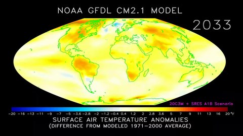
It has been estimated that if greenhouse gas emissions continue at the present rate, Earth's surface temperature could exceed historical values as early as 2047, with potentially harmful
effects on ecosystems, biodiversity and the livelihoods of people worldwide.
[10]
Gases in Earth's atmosphere
Greenhouse gases
Greenhouse gases are those that absorb and emit
infrared radiation in the wavelength range emitted by Earth.
[1] In order, the most abundant greenhouse gases in Earth's atmosphere are:
Atmospheric concentrations of greenhouse gases are determined by the balance between sources (emissions of the gas from human activities and natural systems) and sinks (the removal of the gas from the atmosphere by conversion to a different chemical compound).
[11] The proportion of an emission remaining in the atmosphere after a specified time is the "
airborne fraction" (AF). More precisely, the annual AF is the ratio of the atmospheric increase in a given year to that year's total emissions. For CO
2 the AF over the last 50 years (1956–2006) has been increasing at 0.25 ± 0.21%/year.
[12]
Non-greenhouse gases
Although contributing to many other physical and chemical reactions, the major atmospheric constituents,
nitrogen (
N
2),
oxygen (
O
2), and
argon (Ar), are not greenhouse gases. This is because
molecules containing two atoms of the same element such as
N
2 and
O
2 and
monatomic molecules such as argon (Ar) have no net change in their
dipole moment when they vibrate and hence are almost totally unaffected by
infrared radiation. Although molecules containing two atoms of different elements such as
carbon monoxide (CO) or
hydrogen chloride (HCl) absorb IR, these molecules are short-lived in the atmosphere owing to their reactivity and solubility. Because CO and HCl do not contribute significantly to the greenhouse effect, they are usually omitted when discussing greenhouse gases.
Indirect radiative effects

The false colors in this image represent concentrations of carbon monoxide in the lower atmosphere, ranging from about 390 parts per billion (dark brown pixels), to 220 parts per billion (red pixels), to 50 parts per billion (blue pixels).
[13]
Some gases have indirect radiative effects (whether or not they are greenhouse gases themselves). This happens in two main ways. One way is that when they break down in the atmosphere they produce another greenhouse gas. For example, methane and carbon monoxide (CO) are oxidized to give carbon dioxide (and methane oxidation also produces water vapor; that will be considered below). Oxidation of CO to CO
2 directly produces an unambiguous increase in radiative forcing although the reason is subtle. The peak of the thermal IR emission from Earth's surface is very close to a strong vibrational absorption band of CO
2 (667 cm
−1). On the other hand, the single CO vibrational band only absorbs IR at much higher frequencies (2145 cm
−1), where the ~300 K thermal emission of the surface is at least a factor of ten lower. On the other hand, oxidation of methane to CO
2, which requires reactions with the OH radical, produces an instantaneous reduction, since CO
2 is a weaker greenhouse gas than methane; but it has a longer lifetime. As described below this is not the whole story, since the oxidations of CO and
CH
4 are intertwined by both consuming OH radicals. In any case, the calculation of the total radiative effect needs to include both the direct and indirect forcing.
A second type of indirect effect happens when chemical reactions in the atmosphere involving these gases change the concentrations of greenhouse gases. For example, the destruction of
non-methane volatile organic compounds (NMVOCs) in the atmosphere can produce ozone. The size of the indirect effect can depend strongly on where and when the gas is emitted.
[14]
Methane has a number of indirect effects in addition to forming CO
2. Firstly, the main chemical that destroys methane in the atmosphere is the
hydroxyl radical (OH). Methane reacts with OH and so more methane means that the concentration of OH goes down. Effectively, methane increases its own atmospheric lifetime and therefore its overall radiative effect. The second effect is that the oxidation of methane can produce ozone. Thirdly, as well as making CO
2 the oxidation of methane produces water; this is a major source of water vapor in the
stratosphere, which is otherwise very dry. CO and NMVOC also produce CO
2 when they are oxidized. They remove OH from the atmosphere and this leads to higher concentrations of methane. The surprising effect of this is that the global warming potential of CO is three times that of CO
2.
[15] The same process that converts NMVOC to carbon dioxide can also lead to the formation of tropospheric ozone. Halocarbons have an indirect effect because they destroy stratospheric ozone. Finally
hydrogen can lead to ozone production and
CH
4 increases as well as producing water vapor in the stratosphere.
[14]
Contribution of clouds to Earth's greenhouse effect
The major non-gas contributor to Earth's greenhouse effect,
clouds, also absorb and emit infrared radiation and thus have an effect on radiative properties of the greenhouse gases. Clouds are water droplets or
ice crystals suspended in the atmosphere.
[16][17]
Impacts on the overall greenhouse effect

Schmidt
et al. (2010)
[18] analysed how individual components of the atmosphere contribute to the total greenhouse effect. They estimated that water vapor accounts for about 50% of Earth's greenhouse effect, with clouds contributing 25%, carbon dioxide 20%, and the minor greenhouse gases and
aerosols accounting for the remaining 5%. In the study, the reference model atmosphere is for 1980 conditions. Image credit:
NASA.
[19]
The contribution of each gas to the greenhouse effect is affected by the characteristics of that gas, its abundance, and any indirect effects it may cause. For example, the direct radiative effect of a mass of methane is about 72 times stronger than the same mass of carbon dioxide over a 20-year time frame
[20] but it is present in much smaller concentrations so that its total direct radiative effect is smaller, in part due to its shorter atmospheric lifetime. On the other hand, in addition to its direct radiative impact, methane has a large, indirect radiative effect because it contributes to ozone formation. Shindell
et al. (2005)
[21] argue that the contribution to climate change from methane is at least double previous estimates as a result of this effect.
[22]
When ranked by their direct contribution to the greenhouse effect, the most important are:
[16]
| Compound |
Formula |
Concentration in
atmosphere[23] (ppm) |
Contribution
(%) |
| Water vapor and clouds |
H
2O |
10–50,000(A) |
36–72% |
| Carbon dioxide |
CO2 |
~400 |
9–26% |
| Methane |
CH
4 |
~1.8 |
4–9% |
| Ozone |
O
3 |
2–8(B) |
3–7% |
notes:
(A) Water vapor strongly varies locally[24]
(B) The concentration in stratosphere. About 90% of the ozone in Earth's atmosphere is contained in the stratosphere. |
In addition to the main greenhouse gases listed above, other greenhouse gases include
sulfur hexafluoride,
hydrofluorocarbons and
perfluorocarbons (see
IPCC list of greenhouse gases). Some greenhouse gases are not often listed. For example,
nitrogen trifluoride has a high
global warming potential (GWP) but is only present in very small quantities.
[25]
Proportion of direct effects at a given moment
It is not possible to state that a certain gas causes an exact percentage of the greenhouse effect. This is because some of the gases absorb and emit radiation at the same frequencies as others, so that the total greenhouse effect is not simply the sum of the influence of each gas. The higher ends of the ranges quoted are for each gas alone; the lower ends account for overlaps with the other gases.
[16][17]
In addition, some gases such as methane are known to have large indirect effects that are still being quantified.
[26]
Atmospheric lifetime
Aside from
water vapor, which has a
residence time of about nine days,
[27] major greenhouse gases are well mixed and take many years to leave the atmosphere.
[28] Although it is not easy to know with precision how long it takes greenhouse gases to leave the atmosphere, there are estimates for the principal greenhouse gases. Jacob (1999)
[29] defines the lifetime

of an atmospheric
species X in a one-
box model as the average time that a molecule of X remains in the box. Mathematically
can be defined as the ratio of the mass

(in kg) of X in the box to its removal rate, which is the sum of the flow of X out of the box (

), chemical loss of X (

), and
deposition of X (

) (all in kg/s):

.
[29] If one stopped pouring any of this gas into the box, then after a time
, its concentration would be about halved.
The atmospheric lifetime of a species therefore measures the time required to restore equilibrium following a sudden increase or decrease in its concentration in the atmosphere. Individual atoms or molecules may be lost or deposited to sinks such as the soil, the oceans and other waters, or vegetation and other biological systems, reducing the excess to background concentrations. The average time taken to achieve this is the
mean lifetime.
Carbon dioxide has a variable atmospheric lifetime, and cannot be specified precisely.
[30] The atmospheric lifetime of CO
2 is estimated of the order of 30–95 years.
[31] This figure accounts for CO
2 molecules being removed from the atmosphere by mixing into the ocean, photosynthesis, and other processes. However, this excludes the balancing fluxes of CO
2 into the atmosphere from the geological reservoirs, which have slower characteristic rates.
[32] Although more than half of the CO
2 emitted is removed from the atmosphere within a century, some fraction (about 20%) of emitted CO
2 remains in the atmosphere for many thousands of years.
[33] [34] [35] Similar issues apply to other greenhouse gases, many of which have longer mean lifetimes than CO
2. E.g.,
N2O has a mean atmospheric lifetime of 114 years.
[20]
Radiative forcing
Earth absorbs some of the radiant energy received from the sun, reflects some of it as light and reflects or radiates the rest back to space as
heat.
[36] Earth's surface temperature depends on this balance between incoming and outgoing energy.
[36] If this
energy balance is shifted, Earth's surface could become warmer or cooler, leading to a variety of changes in global climate.
[36]
A number of natural and man-made mechanisms can affect the global energy balance and force changes in Earth's climate.
[36] Greenhouse gases are one such mechanism.
[36] Greenhouse gases in the atmosphere absorb and re-emit some of the outgoing energy radiated from Earth's surface, causing that heat to be retained in the lower atmosphere.
[36] As
explained above, some greenhouse gases remain in the atmosphere for decades or even centuries, and therefore can affect Earth's energy balance over a long time period.
[36] Factors that influence Earth's energy balance can be quantified in terms of "
radiative climate forcing."
[36] Positive radiative forcing indicates warming (for example, by increasing incoming energy or decreasing the amount of energy that escapes to space), whereas negative forcing is associated with cooling.
[36]
Global warming potential
The
global warming potential (GWP) depends on both the efficiency of the molecule as a greenhouse gas and its atmospheric lifetime. GWP is measured relative to the same
mass of CO
2 and evaluated for a specific timescale. Thus, if a gas has a high (positive)
radiative forcing but also a short lifetime, it will have a large GWP on a 20-year scale but a small one on a 100-year scale. Conversely, if a molecule has a longer atmospheric lifetime than CO
2 its GWP will increase with the timescale considered. Carbon dioxide is defined to have a GWP of 1 over all time periods.
Methane has an atmospheric lifetime of 12 ± 3 years. The
2007 IPCC report lists the GWP as 72 over a time scale of 20 years, 25 over 100 years and 7.6 over 500 years.
[20] A 2014 analysis, however, states that although methane's initial impact is about 100 times greater than that of CO
2, because of the shorter atmospheric lifetime, after six or seven decades, the impact of the two gases is about equal, and from then on methane's relative role continues to decline.
[37] The decrease in GWP at longer times is because
methane is degraded to water and CO
2 through chemical reactions in the atmosphere.
Examples of the atmospheric lifetime and
GWP relative to CO
2 for several greenhouse gases are given in the following table:
[20]
The use of
CFC-12 (except some essential uses) has been phased out due to its
ozone depleting properties.
[38] The phasing-out of less active
HCFC-compounds will be completed in 2030.
[39]
Natural and anthropogenic sources
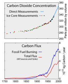
Top: Increasing atmospheric
carbon dioxide levels as measured in the atmosphere and reflected in
ice cores. Bottom: The amount of net carbon increase in the atmosphere, compared to carbon emissions from burning
fossil fuel.

This diagram shows a simplified representation of the contemporary global
carbon cycle. Changes are measured in
gigatons of carbon per year (GtC/y). Canadell
et al. (2007) estimated the growth rate of global average atmospheric CO
2 for 2000–2006 as 1.93 parts-per-million per year (4.1
petagrams of carbon per year).
[43]
Aside from purely human-produced synthetic halocarbons, most greenhouse gases have both natural and human-caused sources. During the pre-industrial
Holocene, concentrations of existing gases were roughly constant. In the industrial era, human activities have added greenhouse gases to the atmosphere, mainly through the burning of fossil fuels and clearing of forests.
[44][45]
The 2007
Fourth Assessment Report compiled by the IPCC (AR4) noted that "changes in atmospheric concentrations of greenhouse gases and aerosols, land cover and solar radiation alter the energy balance of the climate system", and concluded that "increases in anthropogenic greenhouse gas concentrations is very likely to have caused most of the increases in global average temperatures since the mid-20th century".
[46] In AR4, "most of" is defined as more than 50%.
Abbreviations used in the two tables below: ppm = parts-per-million; ppb = parts-per-billion; ppt = parts-per-trillion; W/m2 = watts per square metre
Relevant to radiative forcing and/or ozone depletion; all of the following have no natural sources and hence zero amounts pre-industrial[5]
|
| Gas |
Recent
tropospheric
concentration |
Increased
radiative forcing
(W/m2) |
CFC-11
(trichlorofluoromethane)
(CCl
3F) |
236 ppt /
234 ppt |
0.061 |
CFC-12 (CCl
2F
2) |
527 ppt /
527 ppt |
0.169 |
CFC-113 (Cl
2FC-CClF
2) |
74 ppt /
74 ppt |
0.022 |
HCFC-22 (CHClF
2) |
231 ppt /
210 ppt |
0.046 |
HCFC-141b (CH
3CCl
2F) |
24 ppt /
21 ppt |
0.0036 |
HCFC-142b (CH
3CClF
2) |
23 ppt /
21 ppt |
0.0042 |
Halon 1211 (CBrClF
2) |
4.1 ppt /
4.0 ppt |
0.0012 |
Halon 1301 (CBrClF
3) |
3.3 ppt /
3.3 ppt |
0.001 |
HFC-134a (CH
2FCF
3) |
75 ppt /
64 ppt |
0.0108 |
Carbon tetrachloride (CCl
4) |
85 ppt /
83 ppt |
0.0143 |
Sulfur hexafluoride (SF
6) |
7.79 ppt /[56]
7.39 ppt[56] |
0.0043 |
| Other halocarbons |
Varies by
substance |
collectively
0.02 |
| Halocarbons in total |
|
0.3574 |
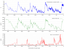
400,000 years of ice core data
Ice cores provide evidence for greenhouse gas concentration variations over the past 800,000 years (see the
following section). Both CO
2 and
CH
4 vary between glacial and interglacial phases, and concentrations of these gases correlate strongly with temperature. Direct data does not exist for periods earlier than those represented in the ice core record, a record that indicates CO
2 mole fractions stayed within a range of 180 ppm to 280 ppm throughout the last 800,000 years, until the increase of the last 250 years. However, various proxies and modeling suggests larger variations in past epochs; 500 million years ago CO
2 levels were likely 10 times higher than now.
[57] Indeed, higher CO
2 concentrations are thought to have prevailed throughout most of the
Phanerozoic eon, with concentrations four to six times current concentrations during the Mesozoic era, and ten to fifteen times current concentrations during the early Palaeozoic era until the middle of the
Devonian period, about 400
Ma.
[58][59][60] The spread of land plants is thought to have reduced CO
2 concentrations during the late Devonian, and plant activities as both sources and sinks of CO
2 have since been important in providing stabilising feedbacks.
[61] Earlier still, a 200-million year period of intermittent, widespread glaciation extending close to the equator (
Snowball Earth) appears to have been ended suddenly, about 550 Ma, by a colossal volcanic outgassing that raised the CO
2 concentration of the atmosphere abruptly to 12%, about 350 times modern levels, causing extreme greenhouse conditions and carbonate deposition as
limestone at the rate of about 1 mm per day.
[62] This episode marked the close of the Precambrian eon, and was succeeded by the generally warmer conditions of the Phanerozoic, during which multicellular animal and plant life evolved. No volcanic carbon dioxide emission of comparable scale has occurred since. In the modern era, emissions to the atmosphere from volcanoes are only about 1% of emissions from human sources.
[62][63][64]
Ice cores
Measurements from Antarctic ice cores show that before industrial emissions started atmospheric CO
2 mole fractions were about 280
parts per million (ppm), and stayed between 260 and 280 during the preceding ten thousand years.
[65] Carbon dioxide mole fractions in the atmosphere have gone up by approximately 35 percent since the 1900s, rising from 280 parts per million by volume to 387 parts per million in 2009. One study using evidence from
stomata of fossilized leaves suggests greater variability, with carbon dioxide mole fractions above 300 ppm during the period seven to ten thousand years ago,
[66] though others have argued that these findings more likely reflect calibration or contamination problems rather than actual CO
2 variability.
[67][68] Because of the way air is trapped in ice (pores in the ice close off slowly to form bubbles deep within the firn) and the time period represented in each ice sample analyzed, these figures represent averages of atmospheric concentrations of up to a few centuries rather than annual or decadal levels.
Changes since the Industrial Revolution

Recent year-to-year increase of atmospheric CO
2.

Major greenhouse gas trends.
Since the beginning of the
Industrial Revolution, the concentrations of most of the greenhouse gases have increased. For example, the mole fraction of carbon dioxide has increased from 280 ppm by about 36% to 380 ppm, or 100 ppm over modern pre-industrial levels. The first 50 ppm increase took place in about 200 years, from the start of the Industrial Revolution to around 1973.
[citation needed]; however the next 50 ppm increase took place in about 33 years, from 1973 to 2006.
[69]
Recent data also shows that the concentration is increasing at a higher rate. In the 1960s, the average annual increase was only 37% of what it was in 2000 through 2007.
[70]
Today, the stock of carbon in the atmosphere increases by more than 3 million tonnes per annum (0.04%) compared with the existing stock.
[clarification needed] This increase is the result of human activities by burning fossil fuels, deforestation and forest degradation in tropical and boreal regions.
[71]
The other greenhouse gases produced from human activity show similar increases in both amount and rate of increase. Many observations are available online in a variety of
Atmospheric Chemistry Observational Databases.
Anthropogenic greenhouse gases
This graph shows changes in the annual greenhouse gas index (AGGI) between 1979 and 2011.
[72] The AGGI measures the levels of greenhouse gases in the atmosphere based on their ability to cause changes in Earth's climate.
[72]
Modern global CO2 emissions from the burning of fossil fuels.
Since about 1750 human activity has increased the concentration of carbon dioxide and other greenhouse gases. Measured atmospheric concentrations of carbon dioxide are currently 100 ppm higher than pre-industrial levels.
[74] Natural sources of carbon dioxide are more than 20 times greater than sources due to human activity,
[75] but over periods longer than a few years natural sources are closely balanced by natural sinks, mainly photosynthesis of carbon compounds by plants and marine plankton. As a result of this balance, the atmospheric mole fraction of carbon dioxide remained between 260 and 280 parts per million for the 10,000 years between the end of the last glacial maximum and the start of the industrial era.
[76]
It is likely that anthropogenic (i.e., human-induced) warming, such as that due to elevated greenhouse gas levels, has had a discernible influence on many physical and biological systems.
[77] Future warming is projected to have a range of
impacts, including
sea level rise,
[78] increased frequencies and severities of some
extreme weather events,
[78] loss of
biodiversity,
[79] and regional changes in
agricultural productivity.
[79]
The main sources of greenhouse gases due to human activity are:
- burning of fossil fuels and deforestation leading to higher carbon dioxide concentrations in the air. Land use change (mainly deforestation in the tropics) account for up to one third of total anthropogenic CO2 emissions.[76]
- livestock enteric fermentation and manure management,[80] paddy rice farming, land use and wetland changes, pipeline losses, and covered vented landfill emissions leading to higher methane atmospheric concentrations. Many of the newer style fully vented septic systems that enhance and target the fermentation process also are sources of atmospheric methane.
- use of chlorofluorocarbons (CFCs) in refrigeration systems, and use of CFCs and halons in fire suppression systems and manufacturing processes.
- agricultural activities, including the use of fertilizers, that lead to higher nitrous oxide (N
2O) concentrations.
The seven sources of CO
2 from fossil fuel combustion are (with percentage contributions for 2000–2004):
[81]
Seven main fossil fuel
combustion sources |
Contribution
(%) |
| Liquid fuels (e.g., gasoline, fuel oil) |
36% |
| Solid fuels (e.g., coal) |
35% |
| Gaseous fuels (e.g., natural gas) |
20% |
| Cement production |
3 % |
| Flaring gas industrially and at wells |
< 1% |
| Non-fuel hydrocarbons |
< 1% |
"International bunker fuels" of transport
not included in national inventories[82] |
4 % |
Carbon dioxide,
methane,
nitrous oxide (
N
2O) and three groups of
fluorinated gases (
sulfur hexafluoride (
SF
6),
hydrofluorocarbons (HFCs), and
perfluorocarbons (PFCs)) are the major anthropogenic greenhouse gases,
[83]:147[84] and are regulated under the
Kyoto Protocol international
treaty, which came into force in 2005.
[85] Emissions limitations specified in the Kyoto Protocol expired in 2012.
[85] The
Cancún agreement, agreed in 2010, includes voluntary pledges made by 76 countries to control emissions.
[86] At the time of the agreement, these 76 countries were collectively responsible for 85% of annual global emissions.
[86]
Although
CFCs are greenhouse gases, they are regulated by the
Montreal Protocol, which was motivated by CFCs' contribution to
ozone depletion rather than by their contribution to global warming. Note that ozone depletion has only a minor role in greenhouse warming though the two processes often are confused in the media.
Tourism[edit]
According to
UNEP global
tourism is closely linked to
climate change. Tourism is a significant contributor to the increasing concentrations of greenhouse gases in the atmosphere. Tourism accounts for about 50% of traffic movements. Rapidly expanding air traffic contributes about 2.5% of the production of CO
2. The number of international travelers is expected to increase from 594 million in 1996 to 1.6 billion by 2020, adding greatly to the problem unless steps are taken to reduce emissions.
[87]
Road Haulage
The road haulage industry plays a part in production of CO
2, contributing around 20% of the UK’s total carbon emissions a year, with only the energy industry having a larger impact at around 39%.
[88] Average carbon emissions within the haulage industry are falling—in the thirty-year period from 1977–2007, the carbon emissions associated with a 200-mile journey fell by 21 percent; NOx emissions are also down 87 percent, whereas journey times have fallen by around a third.
[89] Due to their size, HGVs often receive criticism regarding their CO2 emissions; however, rapid development in engine technology and fuel management is having a largely positive effect.
Role of water vapor

Increasing water vapor in the stratosphere at Boulder, Colorado.
Water vapor accounts for the largest percentage of the greenhouse effect, between 36% and 66% for clear sky conditions and between 66% and 85% when including clouds.
[17] Water vapor concentrations fluctuate regionally, but human activity does not significantly affect water vapor concentrations except at local scales, such as near irrigated fields. The atmospheric concentration of vapor is highly variable and depends largely on temperature, from less than 0.01% in extremely cold regions up to 3% by mass at in saturated air at about 32 °C.
[90] (See
Relative humidity#other important facts.)
The average residence time of a water molecule in the atmosphere is only about nine days, compared to years or centuries for other greenhouse gases such as
CH
4 and CO
2.
[91] Thus, water vapor responds to and amplifies effects of the other greenhouse gases. The
Clausius–Clapeyron relation establishes that more water vapor will be present per unit volume at elevated temperatures. This and other basic principles indicate that warming associated with increased concentrations of the other greenhouse gases also will increase the concentration of water vapor (assuming that the
relative humidity remains approximately constant; modeling and observational studies find that this is indeed so). Because water vapor is a greenhouse gas, this results in further warming and so is a "
positive feedback" that amplifies the original warming. Eventually other earth processes offset these positive feedbacks, stabilizing the global temperature at a new equilibrium and preventing the loss of Earth's water through a Venus-like
runaway greenhouse effect.
[92]
Direct greenhouse gas emissions
Between the period 1970 to 2004, GHG emissions (measured in
CO2-equivalent)
[93] increased at an average rate of 1.6% per year, with CO
2 emissions from the use of fossil fuels growing at a rate of 1.9% per year.
[94][95] Total anthropogenic emissions at the end of 2009 were estimated at 49.5
gigatonnes CO
2-equivalent.
[96]:15 These emissions include CO
2 from fossil fuel use and from land use, as well as emissions of methane, nitrous oxide and other GHGs covered by the
Kyoto Protocol.
At present, the primary source of CO
2 emissions is the burning of
coal,
natural gas, and
petroleum for electricity and heat.
[97]
Regional and national attribution of emissions

This figure shows the relative fraction of anthropogenic greenhouse gases coming from each of eight categories of sources, as estimated by the Emission Database for Global Atmospheric Research version 3.2, fast track 2000 project [1]. These values are intended to provide a snapshot of global annual greenhouse gas emissions in the year 2000. The top panel shows the sum over all anthropogenic greenhouse gases, weighted by their global warming potential over the next 100 years. This consists of 72% carbon dioxide, 18% methane, 8% nitrous oxide and 1% other gases. Lower panels show the comparable information for each of these three primary greenhouse gases, with the same coloring of sectors as used in the top chart. Segments with less than 1% fraction are not labeled.
There are several different ways of measuring GHG emissions, for example, see World Bank (2010)
[98]:362 for tables of national emissions data. Some variables that have been reported
[99] include:
- Definition of measurement boundaries: Emissions can be attributed geographically, to the area where they were emitted (the territory principle) or by the activity principle to the territory produced the emissions. These two principles result in different totals when measuring, for example, electricity importation from one country to another, or emissions at an international airport.
- Time horizon of different GHGs: Contribution of a given GHG is reported as a CO2 equivalent. The calculation to determine this takes into account how long that gas remains in the atmosphere. This is not always known accurately and calculations must be regularly updated to reflect new information.
- What sectors are included in the calculation (e.g., energy industries, industrial processes, agriculture etc.): There is often a conflict between transparency and availability of data.
- The measurement protocol itself: This may be via direct measurement or estimation. The four main methods are the emission factor-based method, mass balance method, predictive emissions monitoring systems, and continuous emissions monitoring systems. These methods differ in accuracy, cost, and usability.
These different measures are sometimes used by different countries to assert various policy/ethical positions on climate change (Banuri
et al., 1996, p. 94).
[100] This use of different measures leads to a lack of comparability, which is problematic when monitoring progress towards targets. There are arguments for the adoption of a common measurement tool, or at least the development of communication between different tools.
[99]
Emissions may be measured over long time periods. This measurement type is called historical or cumulative emissions. Cumulative emissions give some indication of who is responsible for the build-up in the atmospheric concentration of GHGs (IEA, 2007, p. 199).
[101]
The national accounts balance would be positively related to carbon emissions. The national accounts balance shows the difference between exports and imports. For many richer nations, such as the United States, the accounts balance is negative because more goods are imported than they are exported. This is mostly due to the fact that it is cheaper to produce goods outside of developed countries, leading the economies of developed countries to become increasingly dependent on services and not goods. We believed that a positive accounts balance would means that more production was occurring in a country, so more factories working would increase carbon emission levels.(Holtz-Eakin, 1995, pp.;85;101).
[102]
Emissions may also be measured across shorter time periods. Emissions changes may, for example, be measured against a base year of 1990. 1990 was used in the
United Nations Framework Convention on Climate Change (UNFCCC) as the base year for emissions, and is also used in the
Kyoto Protocol (some gases are also measured from the year 1995).
[83]:146,149 A country's emissions may also be reported as a proportion of global emissions for a particular year.
Another measurement is of per capita emissions. This divides a country's total annual emissions by its mid-year population.
[98]:370 Per capita emissions may be based on historical or annual emissions (Banuri
et al., 1996, pp. 106–107).
[100]
Land-use change

Greenhouse gas emissions from agriculture, forestry and other land use, 1970–2010.
Land-use change, e.g., the clearing of forests for agricultural use, can affect the concentration of GHGs in the atmosphere by altering how much carbon flows out of the atmosphere into
carbon sinks.
[103] Accounting for land-use change can be understood as an attempt to measure "net" emissions, i.e., gross emissions from all GHG sources minus the removal of emissions from the atmosphere by carbon sinks (Banuri
et al., 1996, pp. 92–93).
[100]
There are substantial uncertainties in the measurement of net carbon emissions.
[104] Additionally, there is controversy over how carbon sinks should be allocated between different regions and over time (Banuri
et al., 1996, p. 93).
[100] For instance, concentrating on more recent changes in carbon sinks is likely to favour those regions that have deforested earlier, e.g., Europe.
Greenhouse gas intensity

Greenhouse gas intensity in the year 2000, including land-use change.
|

Carbon intensity of GDP (using PPP) for different regions, 1982–2011.
|

Carbon intensity of GDP (using MER) for different regions, 1982–2011.
|
Greenhouse gas intensity is a ratio between greenhouse gas emissions and another metric, e.g., gross domestic product (GDP) or energy use. The terms "carbon intensity" and "
emissions intensity" are also sometimes used.
[105] GHG intensities may be calculated using
market exchange rates (MER) or
purchasing power parity (PPP) (Banuri
et al., 1996, p. 96).
[100] Calculations based on MER show large differences in intensities between developed and developing countries, whereas calculations based on PPP show smaller differences.
Cumulative and historical emissions
Cumulative energy-related CO
2 emissions between the years 1850–2005 grouped into low-income, middle-income, high-income, the
EU-15, and the
OECD countries.
Cumulative energy-related CO2 emissions between the years 1850–2005 for individual countries.
Map of cumulative per capita anthropogenic atmospheric CO2 emissions by country. Cumulative emissions include land use change, and are measured between the years 1950 and 2000.
Regional trends in annual CO2 emissions from fuel combustion between 1971 and 2009.
Regional trends in annual per capita CO2 emissions from fuel combustion between 1971 and 2009.
Cumulative anthropogenic (i.e., human-emitted) emissions of CO
2 from fossil fuel use are a major cause of
global warming,
[106] and give some indication of which countries have contributed most to human-induced climate change.
[107]:15
Top-5 historic CO2 contributors by region over the years 1800 to 1988 (in %)
| Region |
Industrial
CO2 |
Total
CO2 |
| OECD North America |
33.2 |
29.7 |
| OECD Europe |
26.1 |
16.6 |
| Former USSR |
14.1 |
12.5 |
| China |
5.5 |
6.0 |
| Eastern Europe |
5.5 |
4.8 |
The table above to the left is based on Banuri
et al. (1996, p. 94).
[100] Overall, developed countries accounted for 83.8% of industrial CO
2 emissions over this time period, and 67.8% of total CO
2 emissions. Developing countries accounted for industrial CO
2 emissions of 16.2% over this time period, and 32.2% of total CO
2 emissions. The estimate of total CO
2 emissions includes
biotic carbon emissions, mainly from deforestation. Banuri
et al. (1996, p. 94)
[100] calculated per capita cumulative emissions based on then-current population. The ratio in per capita emissions between industrialized countries and developing countries was estimated at more than 10 to 1.
Including biotic emissions brings about the same controversy mentioned earlier regarding carbon sinks and land-use change (Banuri
et al., 1996, pp. 93–94).
[100] The actual calculation of net emissions is very complex, and is affected by how carbon sinks are allocated between regions and the dynamics of the climate system.
Non-
OECD countries accounted for 42% of cumulative energy-related CO
2 emissions between 1890–2007.
[108]:179–180 Over this time period, the US accounted for 28% of emissions; the EU, 23%; Russia, 11%; China, 9%; other OECD countries, 5%; Japan, 4%; India, 3%; and the rest of the world, 18%.
[108]:179–180
Changes since a particular base year
Between 1970–2004, global growth in annual CO
2 emissions was driven by North America, Asia, and the Middle East.
[109] The sharp acceleration in CO
2 emissions since 2000 to more than a 3% increase per year (more than 2 ppm per year) from 1.1% per year during the 1990s is attributable to the lapse of formerly declining trends in
carbon intensity of both developing and developed nations.
China was responsible for most of global growth in emissions during this period. Localised plummeting emissions associated with the collapse of the Soviet Union have been followed by slow emissions growth in this region due to more
efficient energy use, made necessary by the increasing proportion of it that is exported.
[81] In comparison, methane has not increased appreciably, and N
2O by 0.25% y
−1.
Using different base years for measuring emissions has an effect on estimates of national contributions to global warming.
[107]:17–18[110] This can be calculated by dividing a country's highest contribution to global warming starting from a particular base year, by that country's minimum contribution to global warming starting from a particular base year. Choosing between different base years of 1750, 1900, 1950, and 1990 has a significant effect for most countries.
[107]:17–18 Within the
G8 group of countries, it is most significant for the UK, France and Germany. These countries have a long history of CO
2 emissions (see the section on
Cumulative and historical emissions).
Annual emissions[edit]

Per capita anthropogenic greenhouse gas emissions by country for the year 2000 including land-use change.
Annual per capita emissions in the industrialized countries are typically as much as ten times the average in developing countries.
[83]:144 Due to China's fast economic development, its annual per capita emissions are quickly approaching the levels of those in the
Annex I group of the Kyoto Protocol (i.e., the developed countries excluding the USA).
[111] Other countries with fast growing emissions are
South Korea, Iran, and Australia (which apart from the oil rich Persian Gulf states, now has the highest percapita emission rate in the world). On the other hand, annual per capita emissions of the EU-15 and the USA are gradually decreasing over time.
[111] Emissions in Russia and the
Ukraine have decreased fastest since 1990 due to economic restructuring in these countries.
[112]
Energy statistics for fast growing economies are less accurate than those for the industrialized countries. For China's annual emissions in 2008, the
Netherlands Environmental Assessment Agency estimated an uncertainty range of about 10%.
[111]
The
GHG footprint, or greenhouse gas footprint, refers to the amount of GHG that are emitted during the creation of products or services. It is more comprehensive than the commonly used carbon footprint, which measures only carbon dioxide, one of many greenhouse gases.
Top emitter countries[edit]

The top 40 countries emitting all greenhouse gases, showing both that derived from all sources including land clearance and forestry and also the CO2 component excluding those sources. Per capita figures are included. Data taken from
World Resources Institute, Washington. Note that Indonesia and Brazil show very much higher than on graphs simply showing fossil fuel use.
In 2009, the annual top ten emitting countries accounted for about two-thirds of the world's annual energy-related CO
2 emissions.
[113]
Cumulative[edit]
The C-Story of Human Civilization by
PIK
Top-10 cumulative energy-related CO2 emitters between 1850–2008[citation needed]
| Country |
% of world
total |
Metric tonnes
CO2 per person |
| United States |
28.5 |
1,132.7 |
| China |
9.36 |
85.4 |
| Russian Federation |
7.95 |
677.2 |
| Germany |
6.78 |
998.9 |
| United Kingdom |
5.73 |
1,127.8 |
| Japan |
3.88 |
367 |
| France |
2.73 |
514.9 |
| India |
2.52 |
26.7 |
| Canada |
2.17 |
789.2 |
| Ukraine |
2.13 |
556.4 |
Embedded emissions
One way of attributing greenhouse gas (GHG) emissions is to measure the
embedded emissions (also referred to as "embodied emissions") of goods that are being consumed. Emissions are usually measured according to production, rather than consumption.
[114] For example, in the main international
treaty on climate change (the
UNFCCC), countries report on emissions produced within their borders, e.g., the emissions produced from burning fossil fuels.
[108]:179[115]:1 Under a production-based accounting of emissions, embedded emissions on imported goods are attributed to the exporting, rather than the importing, country. Under a consumption-based accounting of emissions, embedded emissions on imported goods are attributed to the importing country, rather than the exporting, country.
Davis and Caldeira (2010)
[115]:4 found that a substantial proportion of CO
2 emissions are traded
internationally. The net effect of trade was to export emissions from China and other emerging markets to consumers in the US, Japan, and Western Europe. Based on annual emissions data from the year 2004, and on a per-capita consumption basis, the top-5 emitting countries were found to be (in tCO
2 per person, per year): Luxembourg (34.7), the US (22.0), Singapore (20.2), Australia (16.7), and Canada (16.6).
[115]:5 Carbon Trust research revealed that approximately 25% of all CO
2 emissions from human activities 'flow' (i.e. are imported or exported) from one country to another. Major developed economies were found to be typically net importers of embodied carbon emissions — with UK consumption emissions 34% higher than production emissions, and Germany (29%), Japan (19%) and the USA (13%) also significant net importers of embodied emissions.
[116]
Effect of policy
Governments have taken action to reduce GHG emissions (
climate change mitigation). Assessments of policy effectiveness have included work by the
Intergovernmental Panel on Climate Change,
[117] International Energy Agency,
[118][119] and
United Nations Environment Programme.
[120] Policies implemented by governments have included
[121][122][123] national and regional targets to reduce emissions, promoting
energy efficiency, and support for
renewable energy such as Solar energy as an effective use of renewable energy because solar uses energy from the sun and does not release pollutants into the air.
Countries and regions listed in Annex I of the
United Nations Framework Convention on Climate Change (UNFCCC) (i.e., the OECD and former planned economies of the Soviet Union) are required to submit periodic assessments to the UNFCCC of actions they are taking to address climate change.
[123]:3 Analysis by the UNFCCC (2011)
[123]:8 suggested that policies and measures undertaken by Annex I Parties may have produced emission savings of 1.5 thousand
Tg CO2-eq in the year 2010, with most savings made in the
energy sector. The projected emissions saving of 1.5 thousand Tg CO
2-eq is measured against a hypothetical "
baseline" of Annex I emissions, i.e., projected Annex I emissions in the absence of policies and measures. The total projected Annex I saving of 1.5 thousand CO
2-eq does not include emissions savings in seven of the Annex I Parties.
[123]:8
Projections
A wide range of projections of future GHG emissions have been produced.
[124] Rogner
et al. (2007)
[125] assessed the scientific literature on GHG projections. Rogner
et al. (2007)
[94] concluded that unless energy policies changed substantially, the world would continue to depend on fossil fuels until 2025–2030. Projections suggest that more than 80% of the world's energy will come from fossil fuels. This conclusion was based on "much evidence" and "high agreement" in the literature.
[94] Projected annual energy-related CO
2 emissions in 2030 were 40–110% higher than in 2000, with two-thirds of the increase originating in developing countries.
[94] Projected annual per capita emissions in developed country regions remained substantially lower (2.8–5.1
tonnes CO
2) than those in developed country regions (9.6–15.1 tonnes CO
2).
[126] Projections consistently showed increase in annual world GHG emissions (the
"Kyoto" gases,
[127] measured in
CO2-equivalent) of 25–90% by 2030, compared to 2000.
[94]
Relative CO2 emission from various fuels
One liter of gasoline, when used as a fuel, produces
2.32 kg (about 1300 liters or 1.3 cubic meters) of carbon dioxide, a greenhouse gas. One US gallon produces 19.4 lb (1,291.5 gallons or 172.65 cubic feet)
[128][129][130]
Life-cycle greenhouse-gas emissions of energy sources
A literature review of numerous energy sources CO
2 emissions by the
IPCC in 2011, found that, the CO
2 emission value that fell within the 50th
percentile of all total life cycle emissions studies conducted was as follows.
[132]
 Play media


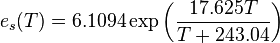
 is the equilibrium or
  is temperature in degrees Celsius). This shows that when atmospheric temperature increases (e.g., due to


.png)
 of an atmospheric
  (in kg) of X in the box to its removal rate, which is the sum of the flow of X out of the box (
 ), chemical loss of X (
 ), and
  ) (all in kg/s):
  .
.


.png)


.png)


_for_different_regions,_1982-2011.png)
_for_different_regions,_1982-2011_(corrected).png)


