Marine conservation

From Wikipedia, the free encyclopedia

https://en.wikipedia.org/wiki/Marine_conservation 

 

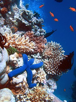
Coral reefs have a great amount of biodiversity.

Marine life
Marine habitats Marine microorganisms Marine microbiomes Marine viruses Marine prokaryotes Marine protists Marine fungi Marine invertebrates Marine vertebrates Marine primary production Marine food web Marine carbon pump Marine biogeochemical cycles Human impact on marine life Marine conservation

Marine conservation, also known as ocean conservation, is the protection and preservation of ecosystems in oceans and seas through planned management in order to prevent the over-exploitation of these resources. Marine conservation is informed by the study of marine plants and animal resources and ecosystem functions and is driven by response to the manifested negative effects seen in the environment such as species loss, habitat degradation and changes in ecosystem functions and focuses on limiting human-caused damage to marine ecosystems, restoring damaged marine ecosystems, and preserving vulnerable species and ecosystems of the marine life. Marine conservation is a relatively new discipline which has developed as a response to biological issues such as extinction and marine habitats change.

Marine conservationists rely on a combination of scientific principles derived from marine biology, Ecology, oceanography, and fisheries science, as well as on human factors, such as demand for marine resources, maritime law, economics, and policy, in order to determine how to best protect and conserve marine species and ecosystems. Marine conservation may be described as a sub-discipline of conservation biology. Marine conservation has been addressed in sustainable development goal 14 that ensures sustainable use of marine resources for sustainable development.

If the oceans die, we all die. – Paul Watson

Coral reefs

Main article: Coral reef

Coral reefs are the epicenter of immense amounts of biodiversity and are a key player in the survival of entire ecosystems. They provide various marine animals with food, protection, and shelter which keep generations of species alive. Furthermore, coral reefs are an integral part of sustaining human life through serving as a food source (i.e., fish and mollusks) as well as a marine space for ecotourism which provides economic benefits. Also, humans are now conducting research regarding the use of corals as new potential sources for pharmaceuticals (i.e. steroids and anti-inflammatory drugs).

Unfortunately, because of the human impact on coral reefs, these ecosystems are becoming increasingly degraded and in need of conservation. The biggest threats include overfishing, destructive fishing practices, sedimentation, and pollution from land-based sources. This, in conjunction with increased carbon in oceans, coral bleaching, and diseases, means that there are no pristine reefs anywhere in the world. Up to 88% of coral reefs in Southeast Asia are now threatened, with 50% of those reefs at either "high" or "very high" risk of disappearing, which directly affects the biodiversity and survival of species dependent on coral.

This is especially harmful to island nations such as Samoa, Indonesia, and the Philippines, because many people there depend on the coral reef ecosystems to feed their families and to make a living. However, many fishermen are unable to catch as many fish as they used to, so they are increasingly using cyanide and dynamite in fishing, which further degrades the coral reef ecosystem. This perpetuation of bad habits simply leads to the further decline of coral reefs and therefore perpetuates the problem. One way of stopping this cycle is by educating the local community about why the conservation of marine spaces that include coral reefs is important.

Human impact

Increasing human populations have resulted in increased human impact on ecosystems. Human activities has resulted in an increased extinction rate of species which has caused a major decrease in biological diversity of plants and animals in our environment. These impacts include increased pressure from fisheries including reef degradation and overfishing as well as pressure from the tourism industry which has increased over the past few years. The deterioration of coral reefs is mainly linked to human activities – 88% of reefs are threatened through various reasons as listed above, including excessive amounts of CO₂ (carbon dioxide) emissions. Oceans absorb approximately 1/3 of the CO₂ produced by humans, which has detrimental effects on the marine environment. The increasing levels of CO₂ in oceans change the seawater chemistry by decreasing the pH, which is known as ocean acidification.

The remains from the Exxon Valdez oil spill after the second treatment by oil spill workers in Alaska

Oil spills also impact marine environments, contributing to marine pollution as a result of human activity. The effects of oil on marine fish have been studied following major spills in the United States.

Shipping is a major vector for the introduction of exotic marine species, some of which can become overabundant and transform ecosystems. Collisions with ships can also be fatal for whales and can impact on the viability of whole populations, including the right whale population off the east coast of the United States.

Overfishing

Overfishing is one of main causes of the decrease in the ocean’s wildlife population over the past years. The Food and Agriculture Organization of the United Nation reported that the percentage of the world's fish stocks that are at biologically sustainable levels have decreased from 90% in 1974 to 65.8% in 2017. The overfishing of these large fisheries destroys the marine environment and threatens the livelihood of billions who depend on fish as protein or as a source of income for catching and selling. 

According to the World Wildlife Fund, illegal, unreported, and unregulated fishing is a major factor in overfishing. Illegal fishing is estimated to account for up to 30% of the catch for some high value species, and the industry is estimated to be worth $36 billion per year.

Overabundance

Overabundance can occur when the population of a certain species cannot be controlled naturally or by human intervention. The domination of one species can create an imbalance in an ecosystem, which can lead to the demise of other species and of the habitat. Overabundance occurs predominately among invasive species.

Introduced species

The international shipping trade has led to the establishment of many marine species beyond their native ranges. Some of these can have adverse consequences, such as the North pacific seastar which was introduced to Tasmania, Australia. Vectors for the translocation of organisms include hull biofouling, the dumping of ballast water and dumping of water from marine aquaria. A tank of ballast water is estimated to contain around 3,000 non-native species. Once established, it is difficult to eradicate an exotic organism from an ecosystem.

The San Francisco Bay is one of the places in the world that is the most impacted by foreign and invasive species. According to the Baykeeper organization, 97 percent of the organisms in the San Francisco Bay have been compromised by the 240 invasive species that have been brought into the ecosystem. Invasive species in the bay such as the Asian clam have changed the food web of the ecosystem by depleting populations of native species such as plankton. The Asian clam clogs pipes and obstructs the flow of water in electrical generating facilities. Their presence in the San Francisco Bay has cost the United States an estimated one billion dollars in damages.

Techniques

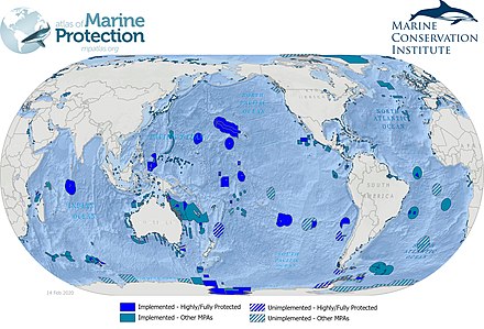
Global marine protected areas as at 2020. Data from MPAtlas

Strategies and techniques for marine conservation tend to combine theoretical disciplines, such as population biology, with practical conservation strategies, such as setting up protected areas, as with marine protected areas (MPAs) or Voluntary Marine Conservation Areas. These protected areas may be established for a variety of reasons and aim to limit the impact of human activity. These protected areas operate differently which includes areas that have seasonal closures and/or permanent closures as well as multiple levels of zoning that allow people to carryout different activities in separate areas; including, speed, no take and multi-use zones. Other techniques include developing sustainable fisheries and restoring the populations of endangered species through artificial means.

Another focus of conservationists is on curtailing human activities that are detrimental to either marine ecosystems or species through policy, techniques such as fishing quotas, like those set up by the Northwest Atlantic Fisheries Organization, or laws such as those listed below. Recognizing the economics involved in human use of marine ecosystems is key, as is education of the public about conservation issues. This includes educating tourists that come to an area who might not be familiar with certain regulations regarding the marine habitat. One example of this is a project called Green Fins based in Southeast Asia that uses the scuba diving industry to educate the public. This project, implemented by UNEP, encourages scuba diving operators to educate their students about the importance of marine conservation and encourage them to dive in an environmentally friendly manner that does not damage coral reefs or associated marine ecosystems.

Scientists divide the process by a few parts, and there are various techniques in each part of it. In marking and capturing, the normal techniques include techniques for restraint in pinnipeds, chemical restraint and immobilization in pinnipeds, techniques for capture-release of cetaceans and techniques for restraint and handling. Recently, some novel approaches include remote sensing techniques to model exposure of coastal-marine ecosystems to riverine flood plumes and advanced iconography.

Techniques also include many social science-based methods. Many researchers have found the effectiveness of marine conservation through change caused by social events and encourage sustainable tourism development to raise the public awareness of it. Researchers suggest integrating customary management into marine conservation and emphasize that practical and conceptual differences exist between customary management and contemporary conservation which have often led to failed attempts to hybridize these systems. Others have suggested to integrate marine conservation and tourism, the establishment of conservation areas can help reduce conflicts. Zoning the protected areas enables the grouping of compatible areas into specific zones and the separation of incompatible areas. Common techniques to raise the general public’s attention also include exposure to the concept of the carbon footprint and to educate people to make sustainable food choices and use fewer plastic products.

Technology and halfway technology

Marine conservation technologies are used to protect endangered and threatened marine organisms and/or habitat. These technologies are innovative and revolutionary because they reduce by-catch, increase the survivorship and health of marine life and habitat, and benefit fishermen who depend on the resources for profit. Examples of technologies include marine protected areas (MPAs), turtle excluder devices (TEDs), autonomous recording unit, pop-up satellite archival tag, and radio-frequency identification (RFID). Commercial practicality plays an important role in the success of marine conservation because it is necessary to cater to the needs of fishermen while also protecting marine life.

Pop-up satellite archival tag (PSAT or PAT) plays a vital role in marine conservation by providing marine biologists with an opportunity to study animals in their natural environments. These are used to track movements of (usually large, migratory) marine animals. A PSAT is an archival tag (or data logger) that is equipped with a means to transmit the collected data via satellite. Though the data are physically stored on the tag, its major advantage is that it does not have to be physically retrieved like an archival tag for the data to be available, making it a viable independent tool for animal behavior studies. These tags have been used to track movements of ocean sunfish, marlin, blue sharks, bluefin tuna, swordfish and sea turtles. Location, depth, temperature, and body movement data are used to answer questions about migratory patterns, seasonal feeding movements, daily habits, and survival after catch and release.

Turtle excluder devices (TEDs) remove a major threat to turtles in their marine environment. Many sea turtles are accidentally captured, injured or killed by fishing. In response to this threat the National Oceanic and Atmospheric Administration (NOAA) worked with the shrimp trawling industry to create the TEDs. By working with the industry they insured the commercial viability of the devices. A TED is a series of bars that is placed at the top or bottom of a trawl net, fitting the bars into the "neck" of the shrimp trawl and acting as a filter to ensure that only small animals may pass through. The shrimp will be caught but larger animals such as marine turtles that become caught by the trawler will be rejected by the filter function of the bars.

Similarly, halfway technologies work to increase the population of marine organisms. However, they do so without behavioral changes, and address the symptoms but not the cause of the declines. Examples of halfway technologies include hatcheries and fish ladders.

Laws and treaties

International laws and treaties related to marine conservation include the 1966 Convention on Fishing and Conservation of Living Resources of the High Seas. United States laws related to marine conservation include the 1972 Marine Mammal Protection Act, as well as the 1972 Marine Protection, Research and Sanctuaries Act, which established the National Marine Sanctuaries program.

In 2010, the Scottish Parliament enacted new legislation for the protection of marine life with the Marine (Scotland) Act 2010. Its provisions include marine planning, marine licensing, marine conservation, seal conservation, and enforcement.

Since 2006, United Nations introduce vulnerable marine ecosystem concept for the management of deep-sea fisheries in the areas beyond national jurisdiction. This concept has been transposed by the European parliament for Atlantic European waters. Additionally, marine conservation is included in the United Nations framework of Sustainable Development Goals (SDGs), most notably SDG 14.

Organizations

The shore of the Pacific Ocean in San Francisco, California

There are marine conservation non-governmental organizations throughout the world that focus on funding conservation efforts, educating the public and stakeholders, and lobbying for conservation law and policy. Examples of these include:

• Ocean Wise (Canada)
• Oceana
• Blue Ventures
• Marine Conservation Society (United Kingdom)
• Fauna and Flora International
• Marine Conservation Institute (United States)
• Blue Frontier Campaign (United States)
• Sea Shepherd Conservation Society (international)
• Community Centered Conservation (C3)
• Reef-World Foundation (United Kingdom)
• Reef Watch (India)
• Marinelife Alliance (Bangladesh)
• Live Ocean (New Zealand)
• ProtectedSeas (United States)
• Australian Marine Conservation Society
• Mission Blue, which leads the Hope Spots initiative
• Zoox (United Kingdom) is an example of an organization that provides both marine conservation training and professional career development to volunteers who are also working on marine conservation projects such as Green Fins.

On a regional level, PERSGA, the Regional Organization for the Conservation of the Environment of the Red Sea and the Gulf of Aden, is a regional entity which serves as the secretariat for the Jeddah Convention-1982, one of the first regional marine agreements. PERSGA member states are Djibouti, Egypt, Jordan, Saudi Arabia, Somalia, Sudan and Yemen.

Prominent campaigns

There have been a number of organized efforts from marine conservation groups such as those aforementioned in this article to raise awareness of the human impact on the situation and inspire people to take action. Some groups take on more public facing campaigns that directly attempt to get civilians engaged with the issue compared to other groups who encourage donations from civilians which goes towards lobbying and advocacy towards the government.

Ocean Conservancy and its International Coastal Cleanup is an example of a public-facing campaign that aims to increase participation in conservation efforts among every day civilians. On a predetermined date every year, Ocean Conservancy promotes The International Coastal Cleanup to rally communities to volunteer to collect trash from the coastlines across the globe. The campaign has expanded originally from its two founders and has now reached over 100 countries.

Oceana is an example of an advocacy/lobbying group that encourages donations as a means to enact legislation and protect the laws of the ocean. Specifically, Oceana is currently lobbying to prevent the expansion of offshore drilling with emphasis in areas such as the Arctic and Belize. Oceana is currently mentioned in a wide range of bills in the US Congress regarding issues such as anti-drilling protections on the Atlantic coast and the penalty for buying, selling, possessing, or transporting shark fins.

Greenpeace is another non-profit organization that seeks to campaign for a healthier environment and more sustainable environmental practices. While the organization addresses a wide range of topics outside of ocean conservation, it is currently focusing in on plastic pollution, sustainable seafood, and protecting the Arctic. They provide information online on their website regarding their current efforts which can help people get connected to the correct resources to make a difference in their community.

Events and initiatives

There have been a wide variety of different events and initiatives to spread the message about the issue.

Events

International Ocean Film Festival

This film festival is the largest ocean destination event according to the MCI. Also known as the IOFF, this event is a four-day film festival that includes over 50 films related to ocean-life around the globe. This event is made to educate viewers and the audience on the environmental issues that are negatively impacting the ocean. Films also include potential solutions to help protect the ocean and environment as well.

Rising Tide Summit

This summit is led by Boardriders Foundation, XPRIZE Foundation, and Marisla Foundation. The summit is more interactive as it provides a panel of speakers as well as a portion for questions and answers. Towards the latter half of the event, companies and individuals are able to participate in a workshop so they can learn more about the benefits of a “blue economy”. This event is centered towards the California population

Initiatives

#SaveOurOceans is a social media campaign that draws NGOs and social media platforms together in the form of a TikTok contest. TikTok has partnered with Conservation International to protect marine life. The #SaveOurOceans campaign was able to reach globally due to influencers spreading the message to a wide audience. Local and global influencers alike played a role in spreading the campaign. TikTok declared that they would donate $2 for every video uploaded with the hashtag, up to $100,000, towards protecting oceans and marine life by reducing plastic waste.

#SuitUpToCleanUp is another social media campaign centered around promoting marine conservation. Launched in August and September of 2018 by Ocean Conservancy, the campaign was intended to inspire participants to clean up pollution in their local waterways. The campaign was meant to coincide with Ocean Conservancy's 33rd Annual International Coastal Cleanup (ICC) on September 15, 2018. The phrase #SuitUpToCleanUp was a way for people to share their stories of how they helped clean up in unique ways.

Extinct and endangered species

Marine mammals

A sleeping monk seal on the sandy beach with the ocean behind it

Baleen whales were predominantly hunted from 1600 through the mid-1900s, and were nearing extinction when a global ban on commercial whaling was put into effect in 1986 by the IWC (International Whaling Convention). The Atlantic gray whale, last sighted in 1740, is now extinct due to European and Native American Whaling. Since the 1960s the global population of monk seals has been rapidly declining. The Hawaiian and Mediterranean monk seals are considered to be one of the most endangered marine mammals on the planet, according to the NOAA. The last sighting of the Caribbean monk seal was in 1952, and it has now been confirmed extinct by the NOAA. The vaquita porpoise, discovered in 1958, has become the most endangered marine species. Over half the population has disappeared since 2012, leaving 100 left in 2014. The vaquita frequently drowns in fishing nets, which are used illegally in marine protected areas off the Gulf of Mexico.

Sea turtles

In 2004, the Marine Turtle Specialist Group (MTSG), from the International Union for Conservation of Nature (IUCN), ran an assessment which determined that green turtles were globally endangered. Population decline in ocean basins is indicated through data collected by the MTSG that analyzes abundance and historical information on the species. This data examined the global population of green turtles at 32 nesting sites, and determined that over the last 100–150 years there has been a 48–65 percent decrease in the number of mature nesting females. The Kemp's ridley sea turtle population fell in 1947 when 33,000 nests, which accounted for 80 percent of the population, were collected and sold by villagers in Racho Nuevo, Mexico. In the early 1960s only 5,000 individuals were left, and between 1978 and 1991, 200 Kemp's Ridley Turtles nested annually. In 2015, the World Wildlife Fund and National Geographic Magazine named the Kemp's ridley the most endangered sea turtle in the world, with 1000 females nesting annually.

Fish

In 2014, the IUCN moved the Pacific bluefin tuna from "least concerned" to "vulnerable" on a scale that represents level of extinction risk. The Pacific bluefin tuna is targeted by the fishing industry mainly for its use in sushi. A stock assessment released in 2013 by the International Scientific Committee for Tuna and Tuna-Like Species in the North Pacific Ocean (ISC) shows that the Pacific bluefin tuna population dropped by 96 percent in the Pacific Ocean. According to the ISC assessment, 90 percent of the Pacific bluefin tuna caught are juveniles that have not reproduced.

Between 2011 and 2014, the European eel, Japanese eel, and American eel were put on the IUCN red list of endangered species. In 2015, the Environmental Agency concluded that the number of European eels has declined by 95 percent since 1990. An Environmental Agency officer, Andy Don, who has been researching eels for the past 20 years, said, "There is no doubt that there is a crisis. People have been reporting catching a kilo of glass eels this year when they would expect to catch 40 kilos. We have got to do something."

Marine plants

A closeup photo of a hand holding a handful of the endangered Johnson's seagrass; a leafy ocean plant

Johnson's seagrass, a food source for the endangered green sea turtle, is the scarcest species in its genus. It reproduces asexually, which limits its ability to populate and colonize habitats. This seagrass is the only marine plant to be listed under the Endangered Species Act , and in 1998, it was granted protection as an endangered species. Data on this species is limited, but it is known that since the 1970s there has been a 50 percent decrease in abundance. There are many reasons behind the decline in the seagrass's proliferation, such as degradation of water quality, careless boating activities, anchoring. In addition to that hurricane activity caused by climate change, increase the risk of extinction of the Johnson's seagrass.

History of marine conservation

Modern marine conservation first became globally recognized in the 1970s after World War II in an era known as the "marine revolution". The United States federal legislation showed its support of marine conservation by institutionalizing protected areas and creating marine estuaries. In the late-1940s the International Union for Conservation of Nature (IUCN)was formed. This program eventually developed into a platform where nations could communicate and make agreements about marine conservation. After the formation of the IUCN, new independent organizations known as non-governmental organizations started to appear. These organizations were self-governed and had individual goals for marine conservation. At the end of the 1970s, undersea explorations equipped with new technology such as computers were undertaken. During these explorations, fundamental principles of change were discovered in relation to marine ecosystems. Through this discovery, the interdependent nature of the ocean was revealed. This led to a change in the approach of marine conservation efforts, and a new emphasis was put on restoring systems within the environment, along with protecting biodiversity.

Life expectancy

From Wikipedia, the free encyclopedia

https://en.wikipedia.org/wiki/Life_expectancy 

Life expectancy at birth, measured by region, between 1950 and 2050

 

Life expectancy by world region, from 1770 to 2018

 

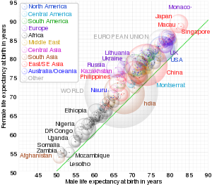
Gender Die Gap: global gender life expectancy gap at birth for countries and territories as defined in the 2018 CIA Factbook, with selected bubbles labelled. The dotted line corresponds to equal female and male life expectancy. The apparent 3D volumes of the bubbles are linearly proportional to their population. (In the SVG file, hover over a bubble to highlight it and show its data.)

Life expectancy is a statistical measure of the average time an organism is expected to live, based on the year of its birth, its current age, and other demographic factors like sex. The most commonly used measure is life expectancy at birth (LEB), which can be defined in two ways. Cohort LEB is the mean length of life of a birth cohort (all individuals born in a given year) and can be computed only for cohorts born so long ago that all their members have died. Period LEB is the mean length of life of a hypothetical cohort assumed to be exposed, from birth through death, to the mortality rates observed at a given year.

National LEB figures reported by national agencies and international organizations for human populations are estimates of period LEB. In the Bronze Age and the Iron Age, human LEB was 26 years; the 2010 world LEB was 67.2 years. In recent years, LEB in Eswatini (Swaziland) is 49, while LEB in Japan is 83. The combination of high infant mortality and deaths in young adulthood from accidents, epidemics, plagues, wars, and childbirth, before modern medicine was widely available, significantly lowers LEB. For example, a society with a LEB of 40 would have relatively few people dying at exactly 40: most will die before 30 or after 55. In populations with high infant mortality rates, LEB is highly sensitive to the rate of death in the first few years of life. Because of this sensitivity, LEB can be grossly misinterpreted, leading to the belief that a population with a low LEB would have a small proportion of older people. A different measure, such as life expectancy at age 5 (e₅), can be used to exclude the effect of infant mortality to provide a simple measure of overall mortality rates other than in early childhood. Aggregate population measures such as the proportion of the population in various age groups, are also used alongside individual-based measures like formal life expectancy when analyzing population structure and dynamics. However, pre-modern societies still had universally higher mortality rates and lower life expectancies at every age for both genders, and this example was relatively rare. In societies with life expectancies of 30, for instance, a 40-year remaining timespan at age 5 may not have been uncommon, but a 60-year one was.

Until the middle of the 20th century, infant mortality was approximately 40–60% of the total mortality. Excluding child mortality, the average life expectancy during the 12th–19th centuries was approximately 55 years. If a medieval person survived childhood, they had about a 50% chance of living 50–55 years, instead of only 25–40 years.

Mathematically, life expectancy is the mean number of years of life remaining at a given age. It is denoted by ${\displaystyle e_{x}}$, which is the mean number of subsequent years of life for someone at age ${\displaystyle x}$, with a particular mortality. Life expectancy, longevity, and maximum lifespan are not synonymous. Longevity refers to the relatively long lifespan of some members of a population. Maximum lifespan is the age at death for the longest-lived individual of a species. Because life expectancy is an average, a particular person may die many years before or many years after the "expected" survival.

Life expectancy is also used in plant or animal ecology, and in life tables (also known as actuarial tables). The concept of life expectancy may also be used in the context of manufactured objects, though the related term shelf life is commonly used for consumer products, and the terms "mean time to breakdown" (MTTB) and "mean time between failures" (MTBF) are used in engineering.

Human patterns

Maximum

Records of human lifespan above age 100 are highly susceptible to errors. For example, the previous world-record holder for human lifespan, Carrie White, was uncovered as a simple typographic error after more than two decades. The longest verified lifespan for any human is that of Frenchwoman Jeanne Calment, who is verified as having lived to age 122 years, 164 days, between 21 February 1875 and 4 August 1997. This is referred to as the "maximum life span," which is the upper boundary of life, the maximum number of years any human is known to have lived. A theoretical study shows that the maximum life expectancy at birth is limited by the human life characteristic value δ, which is around 104 years. According to a study by biologists Bryan G. Hughes and Siegfried Hekimi, there is no evidence for limit on human lifespan. However, this view has been questioned on the basis of error patterns.

Variation over time

Further information: Longevity and List of countries by past life expectancy

The following information is derived from the 1961 Encyclopædia Britannica and other sources, some with questionable accuracy. Unless otherwise stated, it represents estimates of the life expectancies of the world population as a whole. In many instances, life expectancy varied considerably according to class and gender.

Life expectancy at birth takes account of infant mortality and child mortality but not prenatal mortality.

Era	Life expectancy at birth in years	Notes
Paleolithic	22 – 33	Based on the data from modern hunter-gatherer populations, it is estimated that at 15, life expectancy was an additional 39 years (total 54), with a 60% probability of reaching 15.
Neolithic	20 – 33	Based on Early Neolithic data, total life expectancy at 15 would be 28–33 years.
Bronze Age and Iron Age	26	Based on Early and Middle Bronze Age data, total life expectancy at 15 would be 28–36 years.
Classical Greece	25 – 28	Based on Athens Agora and Corinth data, total life expectancy at 15 would be 37–41 years. Most Greeks and Romans died young. About half of all children died before adolescence. Those who survived to the age of 30 had a reasonable chance of reaching 50 or 60. The truly elderly, however, were rare. Because so many died in childhood, life expectancy at birth was probably between 20 and 30 years.
Classical Rome	20–33	Data is lacking, but computer models provide the estimate. If a person survived to age 20, they could expect to live around 30 years more. Life expectancy was probably slightly longer for women than men. When infant mortality is factored out [I.E. counting only the 67-75% who survived the first year], life expectancy is around 34–41 more years [I.E. expected to live to 35–42]. When child mortality is factored out [I.E. counting only the 55-65% who survived to age 5], life expectancy is around 40–45 [I.E. age 45–50]. The ~50% that reached age 10 could also expect to reach ~45-50; at 15 to ~48–54; at 40 to ~60, at 50 to ~64–68; at 60 to ~70–72; at 70 to ~76–77.
Vedic India	25-35	30 was considered the average lifespan by Vedic texts.
Wang clan of China, 1st c. AD – 1749	35	For the 60% that survived the first year [I.E excluding infant mortalities] it rose to ~35.
Early middle ages (Europe, from the late 5th or early 6th century to the 10th century AD)	30–35	Life expectancy for those of both sexes who survived birth averaged about 30–35 years. However, if a Gaulish boy made it past age 20, he might expect to live 25 more years while a woman at age 20 could normally expect about 17 years. And anyone who survived till 40 had a good chance at another 15 to 20 years.
Medieval Islamic world	>35	Average age of scholars was 56–84.3 years.
Pre-Columbian Mesoamerica	>40	The average Aztec life expectancy was 41.2 years for men and 42.1 for women.
Late medieval English peerage	30–33	In Europe, around one-third of infants died in their first year. Once children reached the age of 10, their life expectancy was 32.2 years, and for those who survived to 25, the remaining life expectancy was 23.3 years. Such estimates reflected the life expectancy of adult males from the higher ranks of English society in the Middle Ages, and were similar to that computed for monks of the Christ Church in Canterbury during the 15th century. At age 21, life expectancy of an aristocrat was an additional 43 years (total age 64).
Early modern England (16th - 18th cent.)	33–40	34 years for males in the 18th century. For 15 year old girls: around the 15th & 16th cent it was ~33 years (48 total), and in the 18th it was ~42 (57 total).
18th-century England	25–40	For most of the century it ranged from 35-40; however, in the 20s it dipped as low as 25. For 15 year old girls, it was ~42 (57 total). During the 2nd half of the century it was ~37, while for the elite it passed 40 and approached 50.
Pre-Champlain Canadian Maritimes	60	Samuel de Champlain wrote that in his visits to Mi'kmaq and Huron communities, he met people over 100 years old. Daniel Paul attributes the incredible lifespan in the region to low stress and a healthy diet of lean meats, diverse vegetables and legumes.
18th-century Prussia	24.7	For males.
18th-century France	27.5–30	For males. 24.8 years in 1740—1749, 27.9 years in 1750—1759, 33.9 years in 1800-1809.
18th-century Qing China	39.6	For males. Lavely and Wong (1998, p. 721) show that life expectancy in China was a low of 22 years for the Qing nobility during 1700—1710, 31 years for the same group during 1750—1760, and a high of 46 years for the Tongcheng lineages of Anhui Province during 1960-1709. Zhao (1997a) tabulated the very long series of longevity figures, from 0 C.E. to 1749 C.E., for the Wang clan and found that the life expectancy was 34 years.
18th-century Edo Japan	41.1	For males.
18th-century American colonies	28	Massachusetts colonists who reached the age of 50 could expect to live until 71, and those who were still alive at 60 could to reach 75.
Beginning of the 19th century	~29	Demographic research suggests that at the beginning of the 19th century no country in the world had a life expectancy longer than 40 years. India were ~25, while Belgium was around 40. For Europe as a whole, it was ~33 years.
Early 19th-century England	40	For the 84% who survived the first year [I.E. excluding infant mortality], the average age was ~46 - 48. If they reached 20 it was ~60, if 50 then ~70, if 70 then ~80. For a 15 year old girl it was ~60-65. For the upper-class, LEB rose from ~45 to 50. Another way of thinking about it - less than half of the people born in the mid-19th century made it past their 50th birthday. In contrast, 97% of the people born in 21st century England and Wales can expect to live longer than 50 years.
19th-century British India	25.4
19th-century world average	28.5–32	Over the course of the century: Europe rose from ~33 to 43, the Americas from ~35 to 41, Oceana ~35 to 48, Asia ~28, Africa 26. In 1820s France, LEB was ~38, and for the 80% that survived, it rose to ~47. For Moscow serfs, LEB was ~34, and for the 66% that survived, it rose to ~36. Western Europe in 1830 was ~33 years, while for the people of Hau-Lou in China, it was ~40. The LE for a 10 year-old in Sweden rose from ~44 to ~54.
1900 world average	31–32	Around 48 in Oceana, 43 in Europe, and 41 in the Americas. ~47 in the U.S. Around 48 for 15 year old girls in England.
1950 world average	45.7 – 48	Around 60 years in Europe, North America, Oceania, Japan and parts of South America, but only 41 in Asia and 36 in Africa. Norway had double that with 72, while in Mali it was merely 26.
2019-2020 world average	72.6–73.2	Females: 75.6 years | Males: 70.8 years | Range: ~54 (Central African Republic) - 85.3 Hong Kong

Life expectancy increases with age as the individual survives the higher mortality rates associated with childhood. For instance, the table gives the life expectancy at birth among 13th-century English nobles at 30. Having survived to the age of 21, a male member of the English aristocracy in this period could expect to live:

• 1200–1300: to age 64
• 1300–1400: to age 45 (because of the bubonic plague)
• 1400–1500: to age 69
• 1500–1550: to age 71

17th-century English life expectancy was only about 35 years, largely because infant and child mortality remained high. Life expectancy was under 25 years in the early Colony of Virginia, and in seventeenth-century New England, about 40 percent died before reaching adulthood. During the Industrial Revolution, the life expectancy of children increased dramatically. The under-5 mortality rate in London decreased from 74.5% in 1730–1749 to 31.8% in 1810–1829.

Public health measures are credited with much of the recent increase in life expectancy. During the 20th century, despite a brief drop due to the 1918 flu pandemic starting around that time the average lifespan in the United States increased by more than 30 years, of which 25 years can be attributed to advances in public health.

The life expectancy for people reaching adulthood is greater, — ignoring infant and child mortality. For instance, 16th Century English and Welsh women at 15 years may have had an life expectancy of around 35 more years (50 total).

Regional variations

Further information: List of countries by life expectancy

 

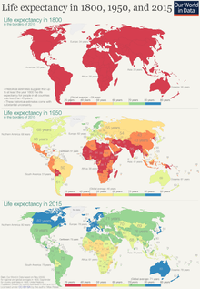
Life expectancy in 1800, 1950, and 2015 – visualization by Our World in Data

Human beings are expected to live on average 30–40 years in Eswatini and 82.6 years in Japan, but the latter's recorded life expectancy may have been very slightly increased by counting many infant deaths as stillborn. An analysis published in 2011 in The Lancet attributes Japanese life expectancy to equal opportunities and public health as well as diet.

Plot of life expectancy vs. GDP per capita in 2009. This phenomenon is known as the Preston curve.

 

Graphs of life expectancy at birth for some sub-Saharan countries showing the fall in the 1990s primarily due to the HIV pandemic.

There are great variations in life expectancy between different parts of the world, mostly caused by differences in public health, medical care, and diet. The impact of AIDS on life expectancy is particularly notable in many African countries. According to projections made by the United Nations (UN) in 2002, the life expectancy at birth for 2010–2015 (if HIV/AIDS did not exist) would have been:

• 70.7 years instead of 31.6 years, Botswana
• 69.9 years instead of 41.5 years, South Africa
• 70.5 years instead of 31.8 years, Zimbabwe

Actual life expectancy in Botswana declined from 65 in 1990 to 49 in 2000 before increasing to 66 in 2011. In South Africa, life expectancy was 63 in 1990, 57 in 2000, and 58 in 2011. And in Zimbabwe, life expectancy was 60 in 1990, 43 in 2000, and 54 in 2011.

During the last 200 years, African countries have generally not had the same improvements in mortality rates that have been enjoyed by countries in Asia, Latin America, and Europe.

In the United States, African-American people have shorter life expectancies than their European-American counterparts. For example, white Americans born in 2010 are expected to live until age 78.9, but black Americans only until age 75.1. This 3.8-year gap, however, is the lowest it has been since 1975 at the latest. The greatest difference was 7.1 years in 1993. In contrast, Asian-American women live the longest of all ethnic groups in the United States, with a life expectancy of 85.8 years. The life expectancy of Hispanic Americans is 81.2 years. According to the new government reports in the US, life expectancy in the country dropped again because of the rise in suicide and drug overdose rates. The Centers for Disease Control (CDC) found nearly 70,000 more Americans died in 2017 than in 2016, with rising rates of death among 25- to 44-year-olds.

Cities also experience a wide range of life expectancy based on neighborhood breakdowns. This is largely due to economic clustering and poverty conditions that tend to associate based on geographic location. Multi-generational poverty found in struggling neighborhoods also contributes. In United States cities such as Cincinnati, the life expectancy gap between low income and high-income neighborhoods touches 20 years.

Economic circumstances

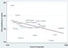
Life expectancy is higher in rich countries with low economic inequality

Economic circumstances also affect life expectancy. For example, in the United Kingdom, life expectancy in the wealthiest and richest areas is several years higher than in the poorest areas. This may reflect factors such as diet and lifestyle, as well as access to medical care. It may also reflect a selective effect: people with chronic life-threatening illnesses are less likely to become wealthy or to reside in affluent areas. In Glasgow, the disparity is amongst the highest in the world: life expectancy for males in the heavily deprived Calton area stands at 54, which is 28 years less than in the affluent area of Lenzie, which is the only 8 km away.

A 2013 study found a pronounced relationship between economic inequality and life expectancy. However, a study by José A. Tapia Granados and Ana Diez Roux at the University of Michigan found that life expectancy actually increased during the Great Depression, and during recessions and depressions in general. The authors suggest that when people are working at a more extreme degree during prosperous economic times, they undergo more stress, exposure to pollution, and the likelihood of injury among other longevity-limiting factors.

Life expectancy is also likely to be affected by exposure to high levels of highway air pollution or industrial air pollution. This is one way that occupation can have a major effect on life expectancy. Coal miners (and in prior generations, asbestos cutters) often have lower life expectancies than average. Other factors affecting an individual's life expectancy are genetic disorders, drug use, tobacco smoking, excessive alcohol consumption, obesity, access to health care, diet, and exercise.

Sex differences

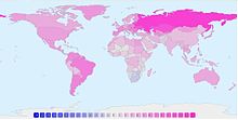
Pink: Countries where females life expectancy at birth is higher than males. Blue: A few countries in the south of Africa where females have shorter lives due to AIDS

In the present, female human life expectancy is greater than that of males, despite females having higher morbidity rates (see Health Survival paradox). There are many potential reasons for this. Traditional arguments tend to favor sociology-environmental factors: historically, men have generally consumed more tobacco, alcohol and drugs than women in most societies, and are more likely to die from many associated diseases such as lung cancer, tuberculosis and cirrhosis of the liver. Men are also more likely to die from injuries, whether unintentional (such as occupational, war or car accidents) or intentional (suicide). Men are also more likely to die from most of the leading causes of death (some already stated above) than women. Some of these in the United States include cancer of the respiratory system, motor vehicle accidents, suicide, cirrhosis of the liver, emphysema, prostate cancer, and coronary heart disease. These far outweigh the female mortality rate from breast cancer and cervical cancer. In the past, mortality rates for females in child-bearing age groups were higher than for males at the same age.

A paper from 2015 found that female fetuses have a higher mortality rate than male fetuses. This finding contradicts papers dating from 2002 and earlier that attribute the male sex to higher in-utero mortality rates. Among the smallest premature babies (those under 2 pounds or 900 g), females have a higher survival rate. At the other extreme, about 90% of individuals aged 110 are female. The difference in life expectancy between men and women in the United States dropped from 7.8 years in 1979 to 5.3 years in 2005, with women expected to live to age 80.1 in 2005. Data from the UK shows the gap in life expectancy between men and women decreasing in later life. This may be attributable to the effects of infant mortality and young adult death rates.

Some argue that shorter male life expectancy is merely another manifestation of the general rule, seen in all mammal species, that larger-sized individuals within a species tend, on average, to have shorter lives. This biological difference occurs because women have more resistance to infections and degenerative diseases.

In her extensive review of the existing literature, Kalben concluded that the fact that women live longer than men was observed at least as far back as 1750 and that, with relatively equal treatment, today males in all parts of the world experience greater mortality than females. Kallen's study, however, was restricted to data in Western Europe alone, where the demographic transition occurred relatively early. United Nations statistics from mid-twentieth century onward, show that in all parts of the world, females have a higher life expectancy at age 60 than males. Of 72 selected causes of death, only 6 yielded greater female than male age-adjusted death rates in 1998 in the United States. Except for birds, for almost all of the animal species studied, males have higher mortality than females. Evidence suggests that the sex mortality differential in people is due to both biological/genetic and environmental/behavioral risk and protective factors.

There is a recent suggestion that mitochondrial mutations that shorten lifespan continue to be expressed in males (but less so in females) because mitochondria are inherited only through the mother. By contrast, natural selection weeds out mitochondria that reduce female survival; therefore such mitochondria are less likely to be passed on to the next generation. This thus suggests that females tend to live longer than males. The authors claim that this is a partial explanation.

In March 2020 researchers reported that their review supports the unguarded X hypothesis: according to this hypothesis one reason for why the average lifespan of males isn't as long as that of females––by 18% on average according to the study––is that they have a Y chromosome which can't protect an individual from harmful genes expressed on the X chromosome, while a duplicate X chromosome, as present in female organisms, can ensure harmful genes aren't expressed.

Before the Industrial Revolution, men lived longer than women on average. In developed countries, starting around 1880, death rates decreased faster among women, leading to differences in mortality rates between males and females. Before 1880 death rates were the same. In people born after 1900, the death rate of 50- to 70-year-old men was double that of women of the same age. Men may be more vulnerable to cardiovascular disease than women, but this susceptibility was evident only after deaths from other causes, such as infections, started to decline. Most of the difference in life expectancy between the sexes is accounted for by differences in the rate of death by cardiovascular diseases among persons aged 50–70.

Genetics

Further information: Genetics of aging

The heritability of lifespan is estimated to be less than 10%, meaning the majority of variation in lifespan is attributable due to differences in environment rather than genetic variation. However, researchers have identified regions of the genome which can influence the length of life and the number of years lived in good health. For example, a genome-wide association study of 1 million lifespans found 12 genetic loci which influenced lifespan by modifying susceptibility to cardiovascular and smoking-related disease. The locus with the largest effect is APOE. Carriers of the APOE ε4 allele live approximately one year less than average (per copy of the ε4 allele), mainly due to increased risk of Alzheimer's disease.

 

"Healthspan, parental lifespan, and longevity are highly genetically correlated"

In July 2020, scientists identified 10 genomic loci with consistent effects across multiple lifespan-related traits, including healthspan, lifespan, and longevity. The genes affected by variation in these loci highlighted haem metabolism as a promising candidate for further research within the field. This study suggests that high levels of iron in the blood likely reduce, and genes involved in metabolising iron likely increase healthy years of life in humans.

A follow-up study which investigated the genetics of frailty and self-rated health in addition to healthspan, lifespan, and longevity also highlighted haem metabolism as an important pathway, and found genetic variants which lower blood protein levels of LPA and VCAM1 were associated with increased healthy lifespan.

Text and images are available under a Creative Commons Attribution 4.0 International License.

Centenarians

Main article: Centenarian

In developed countries, the number of centenarians is increasing at approximately 5.5% per year, which means doubling the centenarian population every 13 years, pushing it from some 455,000 in 2009 to 4.1  million in 2050. Japan is the country with the highest ratio of centenarians (347 for every 1  million inhabitants in September 2010). Shimane Prefecture had an estimated 743 centenarians per million inhabitants.

In the United States, the number of centenarians grew from 32,194 in 1980 to 71,944 in November 2010 (232 centenarians per million inhabitants).

Mental illness

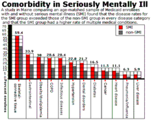
Mental illness is reported to occur in approximately 18% of the average American population.

Life expectancy in the seriously mentally ill is much shorter than the general population.

The mentally ill have been shown to have a 10- to a 25-year reduction in life expectancy. Generally, the reduction of lifespan in the mentally ill population compared to the mentally stable population has been studied and documented.

The greater mortality of people with mental disorders may be due to death from injury, from co-morbid conditions, or medication side effects. For instance, psychiatric medications can increase the risk of developing diabetes. It has been shown that the psychiatric medication olanzapine can increase risk of developing agranulocytosis among other comorbidities. Psychiatric medicines also affect the gastrointestinal tract, where the mentally ill have a four times risk of gastrointestinal disease.

As of the year 2020 and the COVID-19 pandemic, researchers have found an increased risk of death in the mentally ill.

Other illnesses

The life expectancy of people with diabetes, which is 9.3% of the U.S. population, is reduced by roughly ten to twenty years. People over 60 years old with Alzheimer's disease have about a 50% life expectancy of 3 to 10 years. Other demographics that tend to have a lower life expectancy than average include transplant recipients, and the obese.

Education

Education on all levels has been shown to be strongly associated with increased life expectancy. This association may be due partly to higher income, which can lead to increased life expectancy. Despite the association, there is no causal relationship between higher education and life expectancy.

According to a paper from 2015, the mortality rate for the Caucasian population in the United States from 1993 to 2001 is four times higher for those who did not complete high school compared to those who have at least 16 years of education. In fact, within the U.S. adult population, those who have less than a high school education have the shortest life expectancies.

Pre-school education also plays a large role in life expectancy. It was found that high-quality early-stage childhood education had positive effects on health. Researchers discovered this by analyzing the results of the Carolina Abecedarian Project (ABC) finding that the disadvantaged children who were randomly assigned to treatment had lower instances of risk factors for cardiovascular and metabolic diseases in their mid-30s.

Evolution and aging rate

Main article: Life history theory

Various species of plants and animals, including humans, have different lifespans. Evolutionary theory states that organisms that, by virtue of their defenses or lifestyle, live for long periods and avoid accidents, disease, predation, etc. are likely to have genes that code for slow aging, which often translates to good cellular repair. One theory is that if predation or accidental deaths prevent most individuals from living to an old age, there will be less natural selection to increase the intrinsic life span. That finding was supported in a classic study of opossums by Austad; however, the opposite relationship was found in an equally prominent study of guppies by Reznick.

One prominent and very popular theory states that lifespan can be lengthened by a tight budget for food energy called caloric restriction. Caloric restriction observed in many animals (most notably mice and rats) shows a near doubling of life span from a very limited calorific intake. Support for the theory has been bolstered by several new studies linking lower basal metabolic rate to increased life expectancy. That is the key to why animals like giant tortoises can live so long. Studies of humans with life spans of at least 100 have shown a link to decreased thyroid activity, resulting in their lowered metabolic rate.

In a broad survey of zoo animals, no relationship was found between investment of the animal in reproduction and its life span.

Calculation

Further information: Life table § The mathematics

 

A survival tree to explain the calculations of life-expectancy. Red numbers indicate a chance of survival at a specific age, and blue ones indicate age-specific death rates.

The starting point for calculating life expectancy is the age-specific death rates of the population members. If a large amount of data is available, a statistical population can be created that allow the age-specific death rates to be simply taken as the mortality rates actually experienced at each age (the number of deaths divided by the number of years "exposed to risk" in each data cell). However, it is customary to apply smoothing to iron out, as much as possible, the random statistical fluctuations from one year of age to the next. In the past, a very simple model used for this purpose was the Gompertz function, but more sophisticated methods are now used.

These are the most common methods now used for that purpose:

• to fit a mathematical formula, such as an extension of the Gompertz function, to the data.
• for relatively small amounts of data, to look at an established mortality table that was previously derived for a larger population and make a simple adjustment to it (as multiply by a constant factor) to fit the data.
• with a large number of data points, one looks at the mortality rates actually experienced at each age and applies to smooth (as by cubic splines).

While the data required are easily identified in the case of humans, the computation of life expectancy of industrial products and wild animals involves more indirect techniques. The life expectancy and demography of wild animals are often estimated by capturing, marking, and recapturing them. The life of a product, more often termed shelf life, is also computed using similar methods. In the case of long-lived components, such as those used in critical applications: in aircraft, methods like accelerated aging are used to model the life expectancy of a component.

The age-specific death rates are calculated separately for separate groups of data that are believed to have different mortality rates (such as males and females, and perhaps smokers and non-smokers if data are available separately for those groups) and are then used to calculate a life table from which one can calculate the probability of surviving to each age. In actuarial notation, the probability of surviving from age ${\displaystyle x}$ to age ${\displaystyle x+n}$ is denoted ${\displaystyle \,_{n}p_{x}\!}$ and the probability of dying during age ${\displaystyle x}$ (between ages ${\displaystyle x}$ and ${\displaystyle x+1}$) is denoted ${\displaystyle q_{x}\!}$. For example, if 10% of a group of people alive at their 90th birthday die before their 91st birthday, the age-specific death probability at 90 would be 10%. That is a probability, not a mortality rate.

The expected future lifetime of a life age ${\displaystyle x}$ in whole years (the curtate expected lifetime of (x)) is denoted by the symbol ${\displaystyle \,e_{x}\!}$. It is the conditional expected future lifetime (in whole years), assuming survival to age ${\displaystyle x}$. If ${\displaystyle K(x)}$ denotes the curtate future lifetime at ${\displaystyle x}$,

${\displaystyle e_{x}=\operatorname {E} [K(x)]=\sum _{k=0}^{\infty }k\,\Pr(K(x)=k)=\sum _{k=0}^{\infty }k\,\,_{k}p_{x}\,\,q_{x+k}.}$

Substituting ${\displaystyle {}_{k}p_{x}\,q_{x+k}={}_{k}p_{x}-{}_{k+1}p_{x}}$ in the sum and simplifying gives the equivalent formula:${\displaystyle e_{x}=\sum _{k=1}^{\infty }{}\,_{k}p_{x}.}$ If the assumption is made that on average, people live a half year in the year of death, the complete expectation of future lifetime at age ${\displaystyle x}$ is ${\displaystyle e_{x}+1/2}$.

Life expectancy is by definition an arithmetic mean. It can also be calculated by integrating the survival curve from 0 to positive infinity (or equivalently to the maximum lifespan, sometimes called 'omega'). For an extinct or completed cohort (all people born in the year 1850, for example), it can of course simply be calculated by averaging the ages at death. For cohorts with some survivors, it is estimated by using mortality experience in recent years. The estimates are called period cohort life expectancies.

It is important to note that the statistic is usually based on past mortality experience and assumes that the same age-specific mortality rates will continue. Thus, such life expectancy figures need to be adjusted for temporal trends before calculating how long a currently living individual of a particular age is expected to live. Period life expectancy remains a commonly used statistic to summarize the current health status of a population.

However, for some purposes, such as pensions calculations, it is usual to adjust the life table used by assuming that age-specific death rates will continue to decrease over the years, as they have usually done in the past. That is often done by simply extrapolating past trends, but some models exist to account for the evolution of mortality like the Lee–Carter model.

As discussed above, on an individual basis, some factors correlate with longer life. Factors that are associated with variations in life expectancy include family history, marital status, economic status, physique, exercise, diet, drug use including smoking and alcohol consumption, disposition, education, environment, sleep, climate, and health care.

Healthy life expectancy

To assess the quality of these additional years of life, 'healthy life expectancy' has been calculated for the last 30 years. Since 2001, the World Health Organization has published statistics called Healthy life expectancy (HALE), defined as the average number of years that a person can expect to live in "full health" excluding the years lived in less than full health due to disease and/or injury. Since 2004, Eurostat publishes annual statistics called Healthy Life Years (HLY) based on reported activity limitations. The United States uses similar indicators in the framework of the national health promotion and disease prevention plan "Healthy People 2010". More and more countries are using health expectancy indicators to monitor the health of their population.

The long-standing quest for longer life led in the 2010s to a more promising focus on increasing HALE, also known as a person's "healthspan". Besides the benefits of keeping people healthier longer, a goal is to reduce health-care expenses on the many diseases associated with cellular senescence. Approaches being explored include fasting, exercise, and senolytic drugs.

Forecasting

Forecasting life expectancy and mortality form an important subdivision of demography. Future trends in life expectancy have huge implications for old-age support programs like U.S. Social Security and pension since the cash flow in these systems depends on the number of recipients who are still living (along with the rate of return on the investments or the tax rate in pay-as-you-go systems). With longer life expectancies, the systems see increased cash outflow; if the systems underestimate increases in life-expectancies, they will be unprepared for the large payments that will occur, as humans live longer and longer.

Life expectancy forecasting is usually based on two different approaches:

• Forecasting the life expectancy directly, generally using ARIMA or other time-series extrapolation procedures: that has the advantage of simplicity, but it cannot account for changes in mortality at specific ages, and the forecast number cannot be used to derive other life table results. Analyses and forecasts using this approach can be done with any common statistical/mathematical software package, like EViews, R, SAS, Stata, Matlab, or SPSS.
• Forecasting age-specific death rates and computing the life expectancy from the results with life table methods: that is usually more complex than simply forecasting life expectancy because the analyst must deal with correlated age-specific mortality rates, but it seems to be more robust than simple one-dimensional time series approaches. It also yields a set of age specific-rates that may be used to derive other measures, such as survival curves or life expectancies at different ages. The most important approach within this group is the Lee-Carter model, which uses the singular value decomposition on a set of transformed age-specific mortality rates to reduce their dimensionality to a single time series, forecasts that time series and then recovers a full set of age-specific mortality rates from that forecasted value. The software includes Professor Rob J. Hyndman's R package called `demography` and UC Berkeley's LCFIT system.

Policy uses

Life expectancy is one of the factors in measuring the Human Development Index (HDI) of each nation along with adult literacy, education, and standard of living.

Life expectancy is also used in describing the physical quality of life of an area or, for an individual when the value of a life settlement is determined a life insurance policy is sold for a cash asset.

Disparities in life expectancy are often cited as demonstrating the need for better medical care or increased social support. A strongly associated indirect measure is income inequality. For the top 21 industrialized countries, if each person is counted equally, life expectancy is lower in more unequal countries (r = −0.907). There is a similar relationship among states in the US (r = −0.620).

Life expectancy vs. maximum life span

Life expectancy is commonly confused with the average age an adult could expect to live. This confusion may create the expectation that an adult would be unlikely to exceed an average life expectancy, even though, with all statistical probability, an adult, who has already avoided many statistical causes of adolescent mortality, should be expected to outlive the average life expectancy calculated from birth. One must compare the life expectancy of the period after childhood, to estimate the life expectancy of an adult. Life expectancy can change dramatically after childhood, even in preindustrial times as is demonstrated by the Roman Life Expectancy table, which estimates life expectancy to be 25 years at birth, but 53 years upon reaching age 25. Studies like Plymouth Plantation; "Dead at Forty" and Life Expectancy by Age, 1850–2004 similarly show a dramatic increase in life expectancy once adulthood was reached.

Life expectancy differs from maximum life span. Life expectancy is an average for all people in the population — including those who die shortly after birth, those who die in early adulthood (e.g. childbirth, war), and those who live unimpeded until old age. Maximum lifespan is an individual-specific concept — maximum lifespan is, therefore, an upper bound rather than an average. Science author Christopher Wanjek said "has the human race increased its life span? Not at all. This is one of the biggest misconceptions about old age." The maximum life span, or oldest age a human can live, may be constant. Further, there are many examples of people living significantly longer than the average life expectancy of their time period, such as Socrates (71), Saint Anthony the Great (105), Michelangelo (88), and John Adams, 2nd president of the United States (90).

However, anthropologist John D. Hawks criticizes the popular conflation of life span (life expectancy) and maximum life span when popular science writers falsely imply that the average adult human does not live longer than their ancestors. He writes, "[a]ge-specific mortality rates have declined across the adult lifespan. A smaller fraction of adults die at 20, at 30, at 40, at 50, and so on across the lifespan. As a result, we live longer on average... In every way we can measure, human lifespans are longer today than in the immediate past, and longer today than they were 2000 years ago... age-specific mortality rates in adults really have reduced substantially."