From Wikipedia, the free encyclopedia
Entropy production determines the performance of thermal machines such as power plants, heat engines, refrigerators, heat pumps, and air conditioners. It also plays a key role in the thermodynamics of irreversible processes.[1]

The laws of thermodynamics apply to well-defined systems. Fig.1 is a general representation of a thermodynamic system. We consider systems which, in general, are inhomogeneous. Heat and mass are transferred across the boundaries (nonadiabatic, open systems), and the boundaries are moving (usually through pistons). In our formulation we assume that heat and mass transfer and volume changes take place only separately at well-defined regions of the system boundary. The expression, given here, are not the most general formulations of the first and second law. E.g. kinetic energy and potential energy terms are missing and exchange of matter by diffusion is excluded.
The rate of entropy production, denoted by , is a key element of the second law of thermodynamics for open inhomogeneous systems which reads
 enters the system;
  represents the entropy flow into the system at position k, due to matter flowing into the system (
 are the molar flow and mass flow and Smk and sk are the molar entropy (i.e. entropy per mole) and specific entropy (i.e. entropy per unit mass) of the matter, flowing into the system, respectively);
  represents the entropy production rates due to internal processes. The index i in refers to the fact that the entropy is produced due to irreversible processes. The entropy-production rate of every process in nature is always positive or zero. This is an essential aspect of the second law.
The ∑'s indicate the algebraic sum of the respective contributions if there are more heat flows, matter flows, and internal processes.
In order to demonstrate the impact of the second law, and the role of entropy production, it has to be combined with the first law which reads
 the enthalpy flows into the system due to the matter that flows into the system (Hmk its molar enthalpy, hk the specific enthalpy (i.e. enthalpy per unit mass)), and dVk/dt are the rates of change of the volume of the system due to a moving boundary at position k while pk is the pressure behind that boundary; P represents all other forms of power application (such as electrical).
The first and second law have been formulated in terms of time derivatives of U and S rather than in terms of total differentials dU and dS where it is tacitly assumed that dt > 0. So, the formulation in terms of time derivatives is more elegant. An even bigger advantage of this formulation is, however, that it is emphasizes that heat flow and power are the basic thermodynamic properties and that heat and work are derived quantities being the time integrals of the heat flow and the power respectively.

 ) and the volume is fixed (dV/dt = 0). This leads to a significant simplification of the first and second law:
 is the heat supplied at the high temperature TH,
  is the heat removed at ambient temperature Ta, and P is the power delivered by the engine. Eliminating gives
 the performance of the engine is at its maximum and the efficiency is equal to the Carnot efficiency
 at the low temperature TL. Eliminating now gives
the performance of the cooler is at its maximum. The COP is then given by the Carnot Coefficient Of Performance
 which reduces the system performance. This product of ambient temperature and the (average) entropy production rate
  is called the dissipated power.
We first look at a heat engine, assuming that . In other words: the heat flow is completely converted into power. In this case the second law would reduce to
Since and
and  this would result in
  which violates the condition that the entropy production is always positive. Hence: No process is possible in which the sole result is the absorption of heat from a reservoir and its complete conversion into work. This is the Kelvin statement of the second law.
Now look at the case of the refrigerator and assume that the input power is zero. In other words: heat is transported from a low temperature to a high temperature without doing work on the system. The first law with P =0 would give
Since and
and  this would result in which again violates the condition that the entropy production is always positive. Hence: No process is possible whose sole result is the transfer of heat from a body of lower temperature to a body of higher temperature. This is the Clausius statement of the second law.
 from T1 to T2 the rate of entropy production is given by
 from a pressure p1 to p2
 we get
 on (T1-T2) and on (p1-p2) are quadratic. This is typical for expressions of the entropy production rates in general. They guarantee that the entropy production is positive.
 so dS/dt ≥ 0. In other words: the entropy of adiabatic systems can only increase. In equilibrium the entropy is at its maximum. Isolated systems are a special case of adiabatic systems, so this statement is also valid for isolated systems.
Now consider systems with constant temperature and volume. In most cases T is the temperature of the surroundings with which the system is in good thermal contact. Since V is constant the first law gives
 . Substitution in the second law, and using that T is constant, gives
Finally we consider systems with constant temperature and pressure and take P = 0. As p is constant the first laws gives
. As a result the second law, multiplied by T, reduces to
and multiplying with dt gives

Short history
Entropy is produced in irreversible processes. The importance of avoiding irreversible processes (hence reducing the entropy production) was recognized as early as 1824 by Carnot.[2] In 1867 Rudolf Clausius expanded his previous work from 1854[3] on the concept of “unkompensierte Verwandlungen” (uncompensated transformations), which, in our modern nomenclature, would be called the entropy production. In the same article as where he introduced the name entropy,[4] Clausius gives the expression for the entropy production (for a closed system), which he denotes by N, in equation (71) which reads
First and second law

Fig.1 General representation of an inhomogeneous system that consists of a number of subsystems. The interaction of the system with the surroundings is through exchange of heat and other forms of energy, flow of matter, and changes of shape. The internal interactions between the various subsystems are of a similar nature and lead to entropy production.
The laws of thermodynamics apply to well-defined systems. Fig.1 is a general representation of a thermodynamic system. We consider systems which, in general, are inhomogeneous. Heat and mass are transferred across the boundaries (nonadiabatic, open systems), and the boundaries are moving (usually through pistons). In our formulation we assume that heat and mass transfer and volume changes take place only separately at well-defined regions of the system boundary. The expression, given here, are not the most general formulations of the first and second law. E.g. kinetic energy and potential energy terms are missing and exchange of matter by diffusion is excluded.
The rate of entropy production, denoted by
 , is a key element of the second law of thermodynamics for open inhomogeneous systems which reads
 enters the system;
  represents the entropy flow into the system at position k, due to matter flowing into the system (
 are the molar flow and mass flow and Smk and sk are the molar entropy (i.e. entropy per mole) and specific entropy (i.e. entropy per unit mass) of the matter, flowing into the system, respectively);
  represents the entropy production rates due to internal processes. The index i in refers to the fact that the entropy is produced due to irreversible processes. The entropy-production rate of every process in nature is always positive or zero. This is an essential aspect of the second law.
The ∑'s indicate the algebraic sum of the respective contributions if there are more heat flows, matter flows, and internal processes.
In order to demonstrate the impact of the second law, and the role of entropy production, it has to be combined with the first law which reads

 the enthalpy flows into the system due to the matter that flows into the system (Hmk its molar enthalpy, hk the specific enthalpy (i.e. enthalpy per unit mass)), and dVk/dt are the rates of change of the volume of the system due to a moving boundary at position k while pk is the pressure behind that boundary; P represents all other forms of power application (such as electrical).
The first and second law have been formulated in terms of time derivatives of U and S rather than in terms of total differentials dU and dS where it is tacitly assumed that dt > 0. So, the formulation in terms of time derivatives is more elegant. An even bigger advantage of this formulation is, however, that it is emphasizes that heat flow and power are the basic thermodynamic properties and that heat and work are derived quantities being the time integrals of the heat flow and the power respectively.
Examples of irreversible processes
Entropy is produced in irreversible processes. Some important irreversible processes are:- heat flow through a thermal resistance
- fluid flow through a flow resistance such as in the Joule expansion or the Joule-Thomson effect
- diffusion
- chemical reactions
- Joule heating
- friction between solid surfaces
- fluid viscosity within a system.

Fig.2 a: Schematic diagram of a heat engine. A heating power enters the engine at the high temperature TH, and is released at ambient temperature Ta. A power P is produced and the entropy production rate is . b: Schematic diagram of a refrigerator. is the cooling power at the low temperature TL, and is released at ambient temperature. The power P is supplied and is the entropy production rate. The arrows define the positive directions of the flows of heat and power in the two cases. They are positive under normal operating conditions.
 enters the engine at the high temperature TH, and
  is released at ambient temperature Ta. A power P is produced and the entropy production rate is
  . b: Schematic diagram of a refrigerator.
  is the cooling power at the low temperature TL, and is released at ambient temperature. The power P is supplied and is the entropy production rate. The arrows define the positive directions of the flows of heat and power in the two cases. They are positive under normal operating conditions.
Performances of heat engines and refrigerators
Most heat engines and refrigerators are closed cyclic machines.[5] In the steady state the internal energy and the entropy of the machines after one cycle are the same as at the start of the cycle. Hence, on average, dU/dt = 0 and dS/dt = 0 since U and S are functions of state. Furthermore they are closed systems ( ) and the volume is fixed (dV/dt = 0). This leads to a significant simplification of the first and second law:
Engines
For a heat engine (Fig.2a) the first and second law obtain the form
 is the heat supplied at the high temperature TH, is the heat removed at ambient temperature Ta, and P is the power delivered by the engine. Eliminating gives

 the performance of the engine is at its maximum and the efficiency is equal to the Carnot efficiency
Refrigerators
For refrigerators (fig.2b) holds
 at the low temperature TL. Eliminating now gives
 the performance of the cooler is at its maximum. The COP is then given by the Carnot Coefficient Of Performance
Power dissipation
In both cases we find a contribution which reduces the system performance. This product of ambient temperature and the (average) entropy production rate
  is called the dissipated power.
Equivalence with other formulations
It is interesting investigate how the above mathematical formulation of the second law relates with other well-known formulations of the second law.We first look at a heat engine, assuming that
 . In other words: the heat flow is completely converted into power. In this case the second law would reduce to
Since
 and
and  this would result in
  which violates the condition that the entropy production is always positive. Hence: No process is possible in which the sole result is the absorption of heat from a reservoir and its complete conversion into work. This is the Kelvin statement of the second law.
Now look at the case of the refrigerator and assume that the input power is zero. In other words: heat is transported from a low temperature to a high temperature without doing work on the system. The first law with P =0 would give


Since
 and
and  this would result in which again violates the condition that the entropy production is always positive. Hence: No process is possible whose sole result is the transfer of heat from a body of lower temperature to a body of higher temperature. This is the Clausius statement of the second law.
Expressions for the entropy production
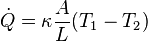
Heat flow
In case of a heat flow from T1 to T2 the rate of entropy production is given by

Flow of matter
In case of a volume flow from a pressure p1 to p2
 we get
 on (T1-T2) and on (p1-p2) are quadratic. This is typical for expressions of the entropy production rates in general. They guarantee that the entropy production is positive.
Entropy of mixing
In this Section we will calculate the entropy of mixing when two ideal gases diffuse into each other. Consider a volume Vt divided in two volumes Va and Vb so that Vt = Va+Vb. The volume Va contains na moles of an ideal gas a and Vb contains nb moles of gas b. The total amount is nt = na+nb. The temperature and pressure in the two volumes is the same. The entropy at the start is given by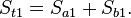


![S_i=-n_tR[x\ln x+(1-x)\ln(1-x)].](http://upload.wikimedia.org/math/2/9/1/29150e208b795022400be4cb01725aac.png)
Joule expansion
The Joule expansion is similar to the mixing described above. It takes place in an adiabatic system consisting of a gas and two rigid vessels (a and b) of equal volume, connected by a valve. Initially the valve is closed. Vessel (a) contains the gas under high pressure while the other vessel (b) is empty. When the valve is opened the gas flows from vessel (a) into (b) until the pressures in the two vessels are equal. The volume, taken by the gas, is doubled while the internal energy of the system is constant (adiabatic and no work done). Assuming that the gas is ideal the molar internal energy is given by Um = CVT. As CV is constant, constant U means constant T. The molar entropy of an ideal gas, as function of the molar volume Vm and T, is given by

Microscopic interpretation
The Joule expansion gives a nice opportunity to explain the entropy production in statistical mechanical (microscopic) terms. At the expansion the volume, that the gas can occupy, is doubled. That means that, for every molecule there are now two possibilities: it can be placed in container an or in b. If we have one mole of gas the number of molecules is equal to Avogadro's number NA. The increase of the microscopic possibilities is a factor 2 per molecule so in total a factor 2NA. Using the well-known Boltzmann expression for the entropy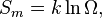

Basic inequalities and stability conditions
In this Section we derive the basic inequalities and stability conditions for closed systems. For closed systems the first law reduces to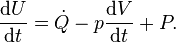
 so dS/dt ≥ 0. In other words: the entropy of adiabatic systems can only increase. In equilibrium the entropy is at its maximum. Isolated systems are a special case of adiabatic systems, so this statement is also valid for isolated systems.
Now consider systems with constant temperature and volume. In most cases T is the temperature of the surroundings with which the system is in good thermal contact. Since V is constant the first law gives
 . Substitution in the second law, and using that T is constant, gives


Finally we consider systems with constant temperature and pressure and take P = 0. As p is constant the first laws gives


Homogeneous systems
In homogeneous systems the temperature and pressure are well-defined and all internal processes are reversible. Hence. As a result the second law, multiplied by T, reduces to
 and multiplying with dt gives


