Omnipotence paradox

From Wikipedia, the free encyclopedia

Detail depicting Averroes, who addressed the omnipotence paradox in the 12th century, from the 14th-century Triunfo de Santo Tomás by Andrea da Firenze (di Bonaiuto)

The omnipotence paradox is a family of paradoxes that arise with some understandings of the term 'omnipotent'. The paradox arises, for example, if one assumes that an omnipotent being has no limits and is capable of realizing any outcome, even logically contradictory ideas such as creating square circles. A no-limits understanding of omnipotence such as this has been rejected by theologians from Thomas Aquinas to contemporary philosophers of religion, such as Alvin Plantinga. Atheological arguments based on the omnipotence paradox are sometimes described as evidence for atheism, though Christian theologians and philosophers, such as Norman Geisler and William Lane Craig, contend that a no-limits understanding of omnipotence is not relevant to orthodox Christian theology. Other possible resolutions to the paradox hinge on the definition of omnipotence applied and the nature of God regarding this application and whether or not omnipotence is directed toward God himself or outward toward his external surroundings.

The omnipotence paradox has medieval origins, dating at least to the 12th century. It was addressed by Averroës and later by Thomas Aquinas. Pseudo-Dionysius the Areopagite (before 532) has a predecessor version of the paradox, asking whether it is possible for God to "deny himself".

The most well-known version of the omnipotence paradox is the so-called paradox of the stone: "Could God create a stone so heavy that even He could not lift it?" This phrasing of the omnipotence paradox is vulnerable to objections based on the physical nature of gravity, such as how the weight of an object depends on what the local gravitational field is. Alternative statements of the paradox that do not involve such difficulties include "If given the axioms of Euclidean geometry, can an omnipotent being create a triangle whose angles do not add up to 180 degrees?" and "Can God create a prison so secure that he cannot escape from it?".

Overview

A common modern version of the omnipotence paradox is expressed in the question: "Can [an omnipotent being] create a stone so heavy that it cannot lift it?" This question generates a dilemma. The being can either create a stone it cannot lift, or it cannot create a stone it cannot lift. If the being can create a stone that it cannot lift, then it seems that it can cease to be omnipotent. If the being cannot create a stone it cannot lift, then it seems it is already not omnipotent.

A related issue is whether the concept of 'logically possible' is different for a world in which omnipotence exists than a world in which omnipotence does not exist.

The dilemma of omnipotence is similar to another classic paradox—the irresistible force paradox: What would happen if an irresistible force were to meet an immovable object? One response to this paradox is to disallow its formulation, by saying that if a force is irresistible, then by definition there is no immovable object; or conversely, if an immovable object exists, then by definition no force can be irresistible. Some claim that the only way out of this paradox is if the irresistible force and immovable object never meet. But this is not a way out, because an object cannot in principle be immovable if a force exists that can in principle move it, regardless of whether the force and the object actually meet.

Types of omnipotence

Peter Geach describes and rejects four levels of omnipotence. He also defines and defends a lesser notion of the "almightiness" of God.

1. "Y is absolutely omnipotent" means that "Y" can do anything that can be expressed in a string of words even if it is self-contradictory: "Y" is not bound by the laws of logic."
2. "Y is omnipotent" means "Y can do X" is true if and only if X is a logically consistent description of a state of affairs. This position was once advocated by Thomas Aquinas. This definition of omnipotence solves some of the paradoxes associated with omnipotence, but some modern formulations of the paradox still work against this definition. Let X = "to make something that its maker cannot lift." As Mavrodes points out there is nothing logically contradictory about this. A man could, for example, make a boat that he could not lift.
3. "Y is omnipotent" means "Y can do X" is true if and only if "Y does X" is logically consistent. Here the idea is to exclude actions that are inconsistent for Y to do but might be consistent for others. Again sometimes it looks as if Aquinas takes this position. Here Mavrodes' worry about X= "to make something its maker cannot lift" is no longer a problem, because "God does X" is not logically consistent. However, this account may still have problems with moral issues like X = "tells a lie" or temporal issues like X = "brings it about that Rome was never founded."
4. "Y is omnipotent" means whenever "Y will bring about X" is logically possible, then "Y can bring about X" is true. This sense, also does not allow the paradox of omnipotence to arise, and unlike definition #3 avoids any temporal worries about whether or not an omnipotent being could change the past. However, Geach criticizes even this sense of omnipotence as misunderstanding the nature of God's promises.
5. "Y is almighty" means that Y is not just more powerful than any creature; no creature can compete with Y in power, even unsuccessfully. In this account nothing like the omnipotence paradox arises, but perhaps that is because God is not taken to be in any sense omnipotent. On the other hand, Anselm of Canterbury seems to think that almightiness is one of the things that make God count as omnipotent.

Augustine of Hippo in his City of God writes "God is called omnipotent on account of His doing what He wills" and thus proposes the definition that "Y is omnipotent" means "If Y wishes to do X then Y can and does do X".

The notion of omnipotence can also be applied to an entity in different ways. An essentially omnipotent being is an entity that is necessarily omnipotent. In contrast, an accidentally omnipotent being is an entity that can be omnipotent for a temporary period of time, and then becomes non-omnipotent. The omnipotence paradox can be applied to each type of being differently.

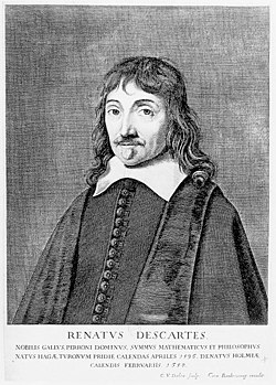
Some Philosophers, such as René Descartes, argue that God is absolutely omnipotent. In addition, some philosophers have considered the assumption that a being is either omnipotent or non-omnipotent to be a false dilemma, as it neglects the possibility of varying degrees of omnipotence. Some modern approaches to the problem have involved semantic debates over whether language—and therefore philosophy—can meaningfully address the concept of omnipotence itself.

Proposed answers

Omnipotence doesn't mean breaking the laws of logic

A common response from Christian philosophers, such as Norman Geisler or William Lane Craig, is that the paradox assumes a wrong definition of omnipotence. Omnipotence, they say, does not mean that God can do anything at all but, rather, that he can do anything that's possible according to his nature. The distinction is important. God cannot perform logical absurdities; he cannot, for instance, make 1+1=3. Likewise, God cannot make a being greater than himself because he is, by definition, the greatest possible being. God is limited in his actions to his nature. The Bible supports this, they assert, in passages such as Hebrews 6:18, which says it is "impossible for God to lie."

Another common response to the omnipotence paradox is to try to define omnipotence to mean something weaker than absolute omnipotence, such as definition 3 or 4 above. The paradox can be resolved by simply stipulating that omnipotence does not require that the being have abilities that are logically impossible, but only be able to do anything that conforms to the laws of logic. A good example of a modern defender of this line of reasoning is George Mavrodes. Essentially, Mavrodes argues that it is no limitation on a being's omnipotence to say that it cannot make a round square. Such a "task" is termed by him a "pseudo-task" as it is self-contradictory and inherently nonsense. Harry Frankfurt—following from Descartes—has responded to this solution with a proposal of his own: that God can create a stone impossible to lift and also lift said stone

For why should God not be able to perform the task in question? To be sure, it is a task—the task of lifting a stone which He cannot lift—whose description is self-contradictory. But if God is supposed capable of performing one task whose description is self-contradictory—that of creating the problematic stone in the first place—why should He not be supposed capable of performing another—that of lifting the stone? After all, is there any greater trick in performing two logically impossible tasks than there is in performing one?

If a being is accidentally omnipotent, it can resolve the paradox by creating a stone it cannot lift, thereby becoming non-omnipotent. Unlike essentially omnipotent entities, it is possible for an accidentally omnipotent being to be non-omnipotent. This raises the question, however, of whether or not the being was ever truly omnipotent, or just capable of great power. On the other hand, the ability to voluntarily give up great power is often thought of as central to the notion of the Christian Incarnation.

If a being is essentially omnipotent, then it can also resolve the paradox (as long as we take omnipotence not to require absolute omnipotence). The omnipotent being is essentially omnipotent, and therefore it is impossible for it to be non-omnipotent. Further, the omnipotent being can do what is logically impossible—just like the accidentally omnipotent—and have no limitations except the inability to become non-omnipotent. The omnipotent being cannot create a stone it cannot lift.

The omnipotent being cannot create such a stone because its power is equal to itself—thus, removing the omnipotence, for there can only be one omnipotent being, but it nevertheless retains its omnipotence. This solution works even with definition 2—as long as we also know the being is essentially omnipotent rather than accidentally so. However, it is possible for non-omnipotent beings to compromise their own powers, which presents the paradox that non-omnipotent beings can do something (to themselves) which an essentially omnipotent being cannot do (to itself). This was essentially the position Augustine of Hippo took in his The City of God:

For He is called omnipotent on account of His doing what He wills, not on account of His suffering what He wills not; for if that should befall Him, He would by no means be omnipotent. Wherefore, He cannot do some things for the very reason that He is omnipotent.

Thus Augustine argued that God could not do anything or create any situation that would, in effect, make God not God.

In a 1955 article in the philosophy journal Mind, J. L. Mackie tried to resolve the paradox by distinguishing between first-order omnipotence (unlimited power to act) and second-order omnipotence (unlimited power to determine what powers to act things shall have). An omnipotent being with both first and second-order omnipotence at a particular time might restrict its own power to act and, henceforth, cease to be omnipotent in either sense. There has been considerable philosophical dispute since Mackie, as to the best way to formulate the paradox of omnipotence in formal logic.

God and logic:

Although the most common translation of the noun "Logos" is "Word" other translations have been used. Gordon Clark (1902–1985), a Calvinist theologian and expert on pre-Socratic philosophy, famously translated Logos as "Logic": "In the beginning was the Logic, and the Logic was with God and the Logic was God." He meant to imply by this translation that the laws of logic were derived from God and formed part of Creation, and were therefore not a secular principle imposed on the Christian world view.
God obeys the laws of logic because God is eternally logical in the same way that God does not perform evil actions because God is eternally good. So, God, by nature logical and unable to violate the laws of logic, cannot make a boulder so heavy he cannot lift it because that would violate the law of non contradiction by creating an immovable object and an unstoppable force.
This raises the question, similar to the Euthyphro Dilemma, of where this law of logic, which God is bound to obey, comes from. According to these theologians (Norman Geisler and William Lane Craig), this law is not a law above God that he assents to but, rather, logic is an eternal part of God's nature, like his omniscience or omnibenevolence.

Paradox is meaningless: the question is sophistry, meaning it makes grammatical sense, but has no intelligible meaning

Another common response is that since God is supposedly omnipotent, the phrase "could not lift" does not make sense and the paradox is meaningless. This may mean that the complexity involved in rightly understanding omnipotence—contra all the logical details involved in misunderstanding it—is a function of the fact that omnipotence, like infinity, is perceived at all by contrasting reference to those complex and variable things, which it is not. An alternative meaning, however, is that a non-corporeal God cannot lift anything, but can raise it (a linguistic pedantry)—or to use the beliefs of Hindus (that there is one God, who can be manifest as several different beings) that whilst it is possible for God to do all things, it is not possible for all his incarnations to do them. As such, God could create a stone so heavy that, in one incarnation, he couldn't lift it, yet could do something that an incarnation that could lift the stone could not.

The lifting a rock paradox (Can God lift a stone larger than he can carry?) uses human characteristics to cover up the main skeletal structure of the question. With these assumptions made, two arguments can stem from it: 

1. Lifting covers up the definition of translation, which means moving something from one point in space to another. With this in mind, the real question would be, "Can God move a rock from one location in space to another that is larger than possible?" For the rock to be unable to move from one space to another, it would have to be larger than space itself. However, it is impossible for a rock to be larger than space, as space always adjusts itself to cover the space of the rock. If the supposed rock was out of space-time dimension, then the question would not make sense—because it would be impossible to move an object from one location in space to another if there is no space to begin with, meaning the faulting is with the logic of the question and not God's capabilities.
2. The words, "Lift a Stone" are used instead to substitute capability. With this in mind, essentially the question is asking if God is incapable, so the real question would be, "Is God capable of being incapable?" If God is capable of being incapable, it means that He is incapable, because He has the potential to not be able to do something. Conversely, if God is incapable of being incapable, then the two inabilities cancel each other out, making God have the capability to do something.

The act of killing oneself is not applicable to an omnipotent being, since, despite that such an act does involve some power, it also involves a lack of power: the human person who can kill himself is already not indestructible, and, in fact, every agent constituting his environment is more powerful in some ways than himself. In other words, all non-omnipotent agents are concretely synthetic: constructed as contingencies of other, smaller, agents, meaning that they, unlike an omnipotent agent, logically can exist not only in multiple instantiation (by being constructed out of the more basic agents they are made of), but are each bound to a different location in space contra transcendent omnipresence. 

Thomas Aquinas asserts that the paradox arises from a misunderstanding of omnipotence. He maintains that inherent contradictions and logical impossibilities do not fall under the omnipotence of God. J. L Cowan sees this paradox as a reason to reject the concept of 'absolute' omnipotence, while others, such as René Descartes, argue that God is absolutely omnipotent, despite the problem.

C. S. Lewis argues that when talking about omnipotence, referencing "a rock so heavy that God cannot lift it" is nonsense just as much as referencing "a square circle"; that it is not logically coherent in terms of power to think that omnipotence includes the power to do the logically impossible. So asking "Can God create a rock so heavy that even he cannot lift it?" is just as much nonsense as asking "Can God draw a square circle?" The logical contradiction here being God's simultaneous ability and disability in lifting the rock: the statement "God can lift this rock" must have a truth value of either true or false, it cannot possess both. This is justified by observing that for the omnipotent agent to create such a stone, it must already be more powerful than itself: such a stone is too heavy for the omnipotent agent to lift, but the omnipotent agent already can create such a stone; If an omnipotent agent already is more powerful than itself, then it already is just that powerful. This means that its power to create a stone that’s too heavy for it to lift is identical to its power to lift that very stone. While this doesn’t quite make complete sense, Lewis wished to stress its implicit point: that even within the attempt to prove that the concept of omnipotence is immediately incoherent, one admits that it is immediately coherent, and that the only difference is that this attempt is forced to admit this despite that the attempt is constituted by a perfectly irrational route to its own unwilling end, with a perfectly irrational set of 'things' included in that end.

In other words, the 'limit' on what omnipotence 'can' do is not a limit on its actual agency, but an epistemological boundary without which omnipotence could not be identified (paradoxically or otherwise) in the first place. In fact, this process is merely a fancier form of the classic Liar Paradox: If I say, "I am a liar", then how can it be true if I am telling the truth therewith, and, if I am telling the truth therewith, then how can I be a liar? So, to think that omnipotence is an epistemological paradox is like failing to recognize that, when taking the statement, 'I am a liar' self-referentially, the statement is reduced to an actual failure to lie. In other words, if one maintains the supposedly 'initial' position that the necessary conception of omnipotence includes the 'power' to compromise both itself and all other identity, and if one concludes from this position that omnipotence is epistemologically incoherent, then one implicitly is asserting that one's own 'initial' position is incoherent. Therefore, the question (and therefore the perceived paradox) is meaningless. Nonsense does not suddenly acquire sense and meaning with the addition of the two words, "God can" before it. Lewis additionally said that, "Unless something is self-evident, nothing can be proved." This implies for the debate on omnipotence that, as in matter, so in the human understanding of truth: it takes no true insight to destroy a perfectly integrated structure, and the effort to destroy has greater effect than an equal effort to build; so, a man is thought a fool who assumes its integrity, and thought an abomination who argues for it. It is easier to teach a fish to swim in outer space than to convince a room full of ignorant fools why it cannot be done.

Language and omnipotence

The philosopher Ludwig Wittgenstein is frequently interpreted as arguing that language is not up to the task of describing the kind of power an omnipotent being would have. In his Tractatus Logico-Philosophicus, he stays generally within the realm of logical positivism until claim 6.4—but at 6.41 and following, he argues that ethics and several other issues are "transcendental" subjects that we cannot examine with language. Wittgenstein also mentions the will, life after death, and God—arguing that, "When the answer cannot be put into words, neither can the question be put into words."

Wittgenstein's work expresses the omnipotence paradox as a problem in semantics—the study of how we give symbols meaning. (The retort "That's only semantics," is a way of saying that a statement only concerns the definitions of words, instead of anything important in the physical world.) According to the Tractatus, then, even attempting to formulate the omnipotence paradox is futile, since language cannot refer to the entities the paradox considers. The final proposition of the Tractatus gives Wittgenstein's dictum for these circumstances: "What we cannot speak of, we must pass over in silence".

Wittgenstein's approach to these problems is influential among other 20th century religious thinkers such as D. Z. Phillips. In his later years, however, Wittgenstein wrote works often interpreted as conflicting with his positions in the Tractatus, and indeed the later Wittgenstein is mainly seen as the leading critic of the early Wittgenstein.

Other versions of the paradox

In the 6th century, Pseudo-Dionysius claims that a version of the omnipotence paradox constituted the dispute between Paul the Apostle and Elymas the Magician mentioned in Acts 13:8, but it is phrased in terms of a debate as to whether or not God can "deny himself" ala 2 Tim 2:13. In the 11th century, Anselm of Canterbury argues that there are many things that God cannot do, but that nonetheless he counts as omnipotent.

Thomas Aquinas advanced a version of the omnipotence paradox by asking whether God could create a triangle with internal angles that did not add up to 180 degrees. As Aquinas put it in Summa contra Gentiles:

Since the principles of certain sciences, such as logic, geometry and arithmetic are taken only from the formal principles of things, on which the essence of the thing depends, it follows that God could not make things contrary to these principles. For example, that a genus was not predicable of the species, or that lines drawn from the centre to the circumference were not equal, or that a triangle did not have three angles equal to two right angles.

This can be done on a sphere, and not on a flat surface. The later invention of non-Euclidean geometry does not resolve this question; for one might as well ask, "If given the axioms of Riemannian geometry, can an omnipotent being create a triangle whose angles do not add up to more than 180 degrees?" In either case, the real question is whether or not an omnipotent being would have the ability to evade consequences that follow logically from a system of axioms that the being created.

A version of the paradox can also be seen in non-theological contexts. A similar problem occurs when accessing legislative or parliamentary sovereignty, which holds a specific legal institution to be omnipotent in legal power, and in particular such an institution's ability to regulate itself.

In a sense, the classic statement of the omnipotence paradox — a rock so heavy that its omnipotent creator cannot lift it — is grounded in Aristotelian science. After all, if we consider the stone's position relative to the sun the planet orbits around, one could hold that the stone is constantly lifted—strained though that interpretation would be in the present context. Modern physics indicates that the choice of phrasing about lifting stones should relate to acceleration; however, this does not in itself of course invalidate the fundamental concept of the generalized omnipotence paradox. However, one could easily modify the classic statement as follows: "An omnipotent being creates a universe that follows the laws of Aristotelian physics. Within this universe, can the omnipotent being create a stone so heavy that the being cannot lift it?"

Ethan Allen's Reason addresses the topics of original sin, theodicy and several others in classic Enlightenment fashion. In Chapter 3, section IV, he notes that "omnipotence itself" could not exempt animal life from mortality, since change and death are defining attributes of such life. He argues, "the one cannot be without the other, any more than there could be a compact number of mountains without valleys, or that I could exist and not exist at the same time, or that God should effect any other contradiction in nature." Labeled by his friends a Deist, Allen accepted the notion of a divine being, though throughout Reason he argues that even a divine being must be circumscribed by logic.

In Principles of Philosophy, Descartes tried refuting the existence of atoms with a variation of this argument, claiming God could not create things so indivisible that he could not divide them.

Dynamic programming

From Wikipedia, the free encyclopedia

Figure 1. Finding the shortest path in a graph using optimal substructure; a straight line indicates a single edge; a wavy line indicates a shortest path between the two vertices it connects (among other paths, not shown, sharing the same two vertices); the bold line is the overall shortest path from start to goal.

Dynamic programming is both a mathematical optimization method and a computer programming method. The method was developed by Richard Bellman in the 1950s and has found applications in numerous fields, from aerospace engineering to economics. In both contexts it refers to simplifying a complicated problem by breaking it down into simpler sub-problems in a recursive manner. While some decision problems cannot be taken apart this way, decisions that span several points in time do often break apart recursively. Likewise, in computer science, if a problem can be solved optimally by breaking it into sub-problems and then recursively finding the optimal solutions to the sub-problems, then it is said to have optimal substructure.

If sub-problems can be nested recursively inside larger problems, so that dynamic programming methods are applicable, then there is a relation between the value of the larger problem and the values of the sub-problems. In the optimization literature this relationship is called the Bellman equation.

Overview

Mathematical optimization

In terms of mathematical optimization, dynamic programming usually refers to simplifying a decision by breaking it down into a sequence of decision steps over time. This is done by defining a sequence of value functions V₁, V₂, ..., V_n taking y as an argument representing the state of the system at times i from 1 to n. The definition of V_n(y) is the value obtained in state y at the last time n. The values V_i at earlier times i = n −1, n − 2, ..., 2, 1 can be found by working backwards, using a recursive relationship called the Bellman equation. For i = 2, ..., n, V_i−1 at any state y is calculated from V_i by maximizing a simple function (usually the sum) of the gain from a decision at time i − 1 and the function V_i at the new state of the system if this decision is made. Since V_i has already been calculated for the needed states, the above operation yields V_i−1 for those states. Finally, V₁ at the initial state of the system is the value of the optimal solution. The optimal values of the decision variables can be recovered, one by one, by tracking back the calculations already performed.

Control theory

In control theory, a typical problem is to find an admissible control ${\displaystyle \mathbf {u} ^{\ast }}$ which causes the system ${\displaystyle {\dot {\mathbf {x} }}(t)=\mathbf {g} \left(\mathbf {x} (t),\mathbf {u} (t),t\right)}$ to follow an admissible trajectory ${\displaystyle \mathbf {x} ^{\ast }}$ on a continuous time interval ${\displaystyle t_{0}\leq t\leq t_{1}}$ that minimizes a cost function

${\displaystyle J=b\left(\mathbf {x} (t_{1}),t_{1}\right)+\int _{t_{0}}^{t_{1}}f\left(\mathbf {x} (t),\mathbf {u} (t),t\right)\mathrm {d} t}$

The solution to this problem is an optimal control law or policy ${\displaystyle \mathbf {u} ^{\ast }=h(\mathbf {x} (t),t)}$, which produces an optimal trajectory ${\displaystyle \mathbf {x} ^{\ast }}$ and an optimized loss function ${\displaystyle J^{\ast }}$. The latter obeys the fundamental equation of dynamic programming:

${\displaystyle -J_{t}^{\ast }=\min _{\mathbf {u} }\left\{f\left(\mathbf {x} (t),\mathbf {u} (t),t\right)+J_{x}^{\ast {\mathsf {T}}}\mathbf {g} \left(\mathbf {x} (t),\mathbf {u} (t),t\right)\right\}}$

a partial differential equation known as the Hamilton–Jacobi–Bellman equation, in which

 ${\displaystyle J_{x}^{\ast }={\frac {\partial J^{\ast }}{\partial \mathbf {x} }}=\left[{\frac {\partial J^{\ast }}{\partial x_{1}}}~~~~{\frac {\partial J^{\ast }}{\partial x_{2}}}~~~~\dots ~~~~{\frac {\partial J^{\ast }}{\partial x_{n}}}\right]^{\mathsf {T}}}$ and ${\displaystyle J_{t}^{\ast }={\frac {\partial J^{\ast }}{\partial t}}}$.

One finds the minimizing ${\displaystyle \mathbf {u} }$ in terms of ${\displaystyle t}$, ${\displaystyle \mathbf {x} }$, and the unknown function ${\displaystyle J_{x}^{\ast }}$ and then substitutes the result into the Hamilton–Jacobi–Bellman equation to get the partial differential equation to be solved with boundary condition ${\displaystyle J\left(t_{1}\right)=b\left(\mathbf {x} (t_{1}),t_{1}\right)}$. In practice, this generally requires numerical techniques for some discrete approximation to the exact optimization relationship.

Alternatively, the continuous process can be approximated by a discrete system, which leads to a following recurrence relation analog to the Hamilton–Jacobi–Bellman equation:

${\displaystyle J_{k}^{\ast }\left(\mathbf {x} _{n-k}\right)=\min _{\mathbf {u} _{n-k}}\left\{{\hat {f}}\left(\mathbf {x} _{n-k},\mathbf {u} _{n-k}\right)+J_{k-1}^{\ast }\left({\hat {g}}\left(\mathbf {x} _{n-k},\mathbf {u} _{n-k}\right)\right)\right\}}$

at the ${\displaystyle k}$-th stage of ${\displaystyle n}$ equally spaced discrete time intervals, and where ${\displaystyle {\hat {f}}}$ and ${\displaystyle {\hat {g}}}$ denote discrete approximations to ${\displaystyle f}$ and ${\displaystyle \mathbf {g} }$. This functional equation is known as the Bellman equation, which can be solved for an exact solution of the discrete approximation of the optimization equation.

Example from economics: Ramsey's problem of optimal saving

In economics, the objective is generally to maximize (rather than minimize) some dynamic social welfare function. In Ramsey's problem, this function relates amounts of consumption to levels of utility. Loosely speaking, the planner faces the trade-off between contemporaneous consumption and future consumption (via investment in capital stock that is used in production), known as intertemporal choice. Future consumption is discounted at a constant rate ${\displaystyle \beta \in (0,1)}$. A discrete approximation to the transition equation of capital is given by

${\displaystyle k_{t+1}={\hat {g}}\left(k_{t},c_{t}\right)=f(k_{t})-c_{t}}$

where ${\displaystyle c}$ is consumption, ${\displaystyle k}$ is capital, and ${\displaystyle f}$ is a production function satisfying the Inada conditions. An initial capital stock ${\displaystyle k_{0}>0}$ is assumed.

Let ${\displaystyle c_{t}}$ be consumption in period t, and assume consumption yields utility ${\displaystyle u(c_{t})=\ln(c_{t})}$ as long as the consumer lives. Assume the consumer is impatient, so that he discounts future utility by a factor b each period, where ${\displaystyle 0$ . Let ${\displaystyle k_{t}}$ be capital in period t. Assume initial capital is a given amount ${\displaystyle k_{0}>0}$, and suppose that this period's capital and consumption determine next period's capital as ${\displaystyle k_{t+1}=Ak_{t}^{a}-c_{t}}$, where A is a positive constant and ${\displaystyle 0$. Assume capital cannot be negative. Then the consumer's decision problem can be written as follows:

${\displaystyle \max \sum _{t=0}^{T}b^{t}\ln(c_{t})}$ subject to ${\displaystyle k_{t+1}=Ak_{t}^{a}-c_{t}\geq 0}$ for all ${\displaystyle t=0,1,2,\ldots ,T}$

Written this way, the problem looks complicated, because it involves solving for all the choice variables ${\displaystyle c_{0},c_{1},c_{2},\ldots ,c_{T}}$. (Note that ${\displaystyle k_{0}}$ is not a choice variable—the consumer's initial capital is taken as given.)

The dynamic programming approach to solve this problem involves breaking it apart into a sequence of smaller decisions. To do so, we define a sequence of value functions ${\displaystyle V_{t}(k)}$, for ${\displaystyle t=0,1,2,\ldots ,T,T+1}$ which represent the value of having any amount of capital k at each time t. Note that ${\displaystyle V_{T+1}(k)=0}$, that is, there is (by assumption) no utility from having capital after death.

The value of any quantity of capital at any previous time can be calculated by backward induction using the Bellman equation. In this problem, for each ${\displaystyle t=0,1,2,\ldots ,T}$, the Bellman equation is

${\displaystyle V_{t}(k_{t})\,=\,\max \left(\ln(c_{t})+bV_{t+1}(k_{t+1})\right)}$ subject to ${\displaystyle k_{t+1}=Ak_{t}^{a}-c_{t}\geq 0}$
This problem is much simpler than the one we wrote down before, because it involves only two decision variables, ${\displaystyle c_{t}}$ and ${\displaystyle k_{t+1}}$. Intuitively, instead of choosing his whole lifetime plan at birth, the consumer can take things one step at a time. At time t, his current capital ${\displaystyle k_{t}}$ is given, and he only needs to choose current consumption ${\displaystyle c_{t}}$ and saving ${\displaystyle k_{t+1}}$.

To actually solve this problem, we work backwards. For simplicity, the current level of capital is denoted as k. ${\displaystyle V_{T+1}(k)}$ is already known, so using the Bellman equation once we can calculate ${\displaystyle V_{T}(k)}$, and so on until we get to ${\displaystyle V_{0}(k)}$, which is the value of the initial decision problem for the whole lifetime. In other words, once we know ${\displaystyle V_{T-j+1}(k)}$, we can calculate ${\displaystyle V_{T-j}(k)}$, which is the maximum of ${\displaystyle \ln(c_{T-j})+bV_{T-j+1}(Ak^{a}-c_{T-j})}$, where ${\displaystyle c_{T-j}}$ is the choice variable and ${\displaystyle Ak^{a}-c_{T-j}\geq 0}$.

Working backwards, it can be shown that the value function at time ${\displaystyle t=T-j}$ is

${\displaystyle V_{T-j}(k)\,=\,a\sum _{i=0}^{j}a^{i}b^{i}\ln k+v_{T-j}}$

where each ${\displaystyle v_{T-j}}$ is a constant, and the optimal amount to consume at time ${\displaystyle t=T-j}$ is

${\displaystyle c_{T-j}(k)\,=\,{\frac {1}{\sum _{i=0}^{j}a^{i}b^{i}}}Ak^{a}}$

which can be simplified to

${\displaystyle {\begin{aligned}c_{T}(k)&=Ak^{a}\\c_{T-1}(k)&={\frac {Ak^{a}}{1+ab}}\\c_{T-2}(k)&={\frac {Ak^{a}}{1+ab+a^{2}b^{2}}}\\&\dots \\c_{2}(k)&={\frac {Ak^{a}}{1+ab+a^{2}b^{2}+\ldots +a^{T-2}b^{T-2}}}\\c_{1}(k)&={\frac {Ak^{a}}{1+ab+a^{2}b^{2}+\ldots +a^{T-2}b^{T-2}+a^{T-1}b^{T-1}}}\\c_{0}(k)&={\frac {Ak^{a}}{1+ab+a^{2}b^{2}+\ldots +a^{T-2}b^{T-2}+a^{T-1}b^{T-1}+a^{T}b^{T}}}\end{aligned}}}$

We see that it is optimal to consume a larger fraction of current wealth as one gets older, finally consuming all remaining wealth in period T, the last period of life.

Computer programming

There are two key attributes that a problem must have in order for dynamic programming to be applicable: optimal substructure and overlapping sub-problems. If a problem can be solved by combining optimal solutions to non-overlapping sub-problems, the strategy is called "divide and conquer" instead. This is why merge sort and quick sort are not classified as dynamic programming problems.

Optimal substructure means that the solution to a given optimization problem can be obtained by the combination of optimal solutions to its sub-problems. Such optimal substructures are usually described by means of recursion. For example, given a graph G=(V,E), the shortest path p from a vertex u to a vertex v exhibits optimal substructure: take any intermediate vertex w on this shortest path p. If p is truly the shortest path, then it can be split into sub-paths p₁ from u to w and p₂ from w to v such that these, in turn, are indeed the shortest paths between the corresponding vertices. Hence, one can easily formulate the solution for finding shortest paths in a recursive manner, which is what the Bellman–Ford algorithm or the Floyd–Warshall algorithm does.

Overlapping sub-problems means that the space of sub-problems must be small, that is, any recursive algorithm solving the problem should solve the same sub-problems over and over, rather than generating new sub-problems. For example, consider the recursive formulation for generating the Fibonacci series: F_i = F_i−1 + F_i−2, with base case F₁ = F₂ = 1. Then F₄₃ = F₄₂ + F₄₁, and F₄₂ = F₄₁ + F₄₀. Now F₄₁ is being solved in the recursive sub-trees of both F₄₃ as well as F₄₂. Even though the total number of sub-problems is actually small (only 43 of them), we end up solving the same problems over and over if we adopt a naive recursive solution such as this. Dynamic programming takes account of this fact and solves each sub-problem only once.

Figure 2. The subproblem graph for the Fibonacci sequence. The fact that it is not a tree indicates overlapping subproblems.

This can be achieved in either of two ways:

1. Top-down approach: This is the direct fall-out of the recursive formulation of any problem. If the solution to any problem can be formulated recursively using the solution to its sub-problems, and if its sub-problems are overlapping, then one can easily memorize or store the solutions to the sub-problems in a table. Whenever we attempt to solve a new sub-problem, we first check the table to see if it is already solved. If a solution has been recorded, we can use it directly, otherwise we solve the sub-problem and add its solution to the table;
2. Bottom-up approach: Once we formulate the solution to a problem recursively as in terms of its sub-problems, we can try reformulating the problem in a bottom-up fashion: try solving the sub-problems first and use their solutions to build-on and arrive at solutions to bigger sub-problems. This is also usually done in a tabular form by iteratively generating solutions to bigger and bigger sub-problems by using the solutions to small sub-problems. For example, if we already know the values of F₄₁ and F₄₀, we can directly calculate the value of F₄₂.

Some programming languages can automatically memoize the result of a function call with a particular set of arguments, in order to speed up call-by-name evaluation (this mechanism is referred to as call-by-need). Some languages make it possible portably (e.g. Scheme, Common Lisp or Perl). Some languages have automatic memoization built in, such as tabled Prolog and J, which supports memoization with the M. adverb. In any case, this is only possible for a referentially transparent function. Memoization is also encountered as an easily accessible design pattern within term-rewrite based languages such as Wolfram Language.

Bioinformatics

Dynamic programming is widely used in bioinformatics for the tasks such as sequence alignment, protein folding, RNA structure prediction and protein-DNA binding. The first dynamic programming algorithms for protein-DNA binding were developed in the 1970s independently by Charles DeLisi in USA and Georgii Gurskii and Alexander Zasedatelev in USSR. Recently these algorithms have become very popular in bioinformatics and computational biology, particularly in the studies of nucleosome positioning and transcription factor binding.

Examples: Computer algorithms

Dijkstra's algorithm for the shortest path problem

From a dynamic programming point of view, Dijkstra's algorithm for the shortest path problem is a successive approximation scheme that solves the dynamic programming functional equation for the shortest path problem by the Reaching method.

In fact, Dijkstra's explanation of the logic behind the algorithm, namely

Problem 2. Find the path of minimum total length between two given nodes ${\displaystyle P}$ and ${\displaystyle Q}$.
We use the fact that, if ${\displaystyle R}$ is a node on the minimal path from ${\displaystyle P}$ to ${\displaystyle Q}$, knowledge of the latter implies the knowledge of the minimal path from ${\displaystyle P}$ to ${\displaystyle R}$.

This is a paraphrasing of Bellman's famous Principle of Optimality in the context of the shortest path problem.

Fibonacci sequence

Here is a naïve implementation of a function finding the nth member of the Fibonacci sequence, based directly on the mathematical definition:

function fib(n)
  if n <= 1 return n
   return fib(n − 1) + fib(n − 2)

Notice that if we call, say, fib(5), we produce a call tree that calls the function on the same value many different times:

1. fib(5)
2. fib(4) + fib(3)
3. (fib(3) + fib(2)) + (fib(2) + fib(1))
4. ((fib(2) + fib(1)) + (fib(1) + fib(0))) + ((fib(1) + fib(0)) + fib(1))
5. (((fib(1) + fib(0)) + fib(1)) + (fib(1) + fib(0))) + ((fib(1) + fib(0)) + fib(1))

In particular, fib(2) was calculated three times from scratch. In larger examples, many more values of fib, or subproblems, are recalculated, leading to an exponential time algorithm.

Now, suppose we have a simple map object, m, which maps each value of fib that has already been calculated to its result, and we modify our function to use it and update it. The resulting function requires only O(n) time instead of exponential time (but requires O(n) space):

var m := map(0 → 0, 1 → 1)
function fib(n)
  if key n is not in map m 
    m[n] := fib(n − 1) + fib(n − 2)
  return m[n]

This technique of saving values that have already been calculated is called memoization; this is the top-down approach, since we first break the problem into subproblems and then calculate and store values.

In the bottom-up approach, we calculate the smaller values of fib first, then build larger values from them. This method also uses O(n) time since it contains a loop that repeats n − 1 times, but it only takes constant (O(1)) space, in contrast to the top-down approach which requires O(n) space to store the map.

function fib(n)
  if n = 0
    return 0
  else
    var previousFib := 0, currentFib := 1
    repeat n − 1 times // loop is skipped if n = 1
      var newFib := previousFib + currentFib
          previousFib := currentFib
          currentFib  := newFib
      return currentFib

In both examples, we only calculate fib(2) one time, and then use it to calculate both fib(4) and fib(3), instead of computing it every time either of them is evaluated.

Note that the above method actually takes ${\displaystyle \Omega (n^{2})}$ time for large n because addition of two integers with ${\displaystyle \Omega (n)}$ bits each takes ${\displaystyle \Omega (n)}$ time. (The n^th fibonacci number has ${\displaystyle \Omega (n)}$ bits.) Also, there is a closed form for the Fibonacci sequence, known as Binet's formula, from which the ${\displaystyle n}$-th term can be computed in approximately ${\displaystyle O(n(\log n)^{2})}$ time, which is more efficient than the above dynamic programming technique. However, the simple recurrence directly gives the matrix form that leads to an approximately ${\displaystyle O(n\log n)}$ algorithm by fast matrix exponentiation.

A type of balanced 0–1 matrix

Consider the problem of assigning values, either zero or one, to the positions of an n × n matrix, with n even, so that each row and each column contains exactly n / 2 zeros and n / 2 ones. We ask how many different assignments there are for a given ${\displaystyle n}$. For example, when n = 4, four possible solutions are

${\displaystyle {\begin{bmatrix}0&1&0&1\\1&0&1&0\\0&1&0&1\\1&0&1&0\end{bmatrix}}{\text{ and }}{\begin{bmatrix}0&0&1&1\\0&0&1&1\\1&1&0&0\\1&1&0&0\end{bmatrix}}{\text{ and }}{\begin{bmatrix}1&1&0&0\\0&0&1&1\\1&1&0&0\\0&0&1&1\end{bmatrix}}{\text{ and }}{\begin{bmatrix}1&0&0&1\\0&1&1&0\\0&1&1&0\\1&0&0&1\end{bmatrix}}.}$

There are at least three possible approaches: brute force, backtracking, and dynamic programming.

Brute force consists of checking all assignments of zeros and ones and counting those that have balanced rows and columns (n / 2 zeros and n / 2 ones). As there are ${\displaystyle {\tbinom {n}{n/2}}^{n}}$ possible assignments, this strategy is not practical except maybe up to ${\displaystyle n=6}$.

Backtracking for this problem consists of choosing some order of the matrix elements and recursively placing ones or zeros, while checking that in every row and column the number of elements that have not been assigned plus the number of ones or zeros are both at least n / 2. While more sophisticated than brute force, this approach will visit every solution once, making it impractical for n larger than six, since the number of solutions is already 116,963,796,250 for n = 8.

Dynamic programming makes it possible to count the number of solutions without visiting them all. Imagine backtracking values for the first row – what information would we require about the remaining rows, in order to be able to accurately count the solutions obtained for each first row value? We consider k × n boards, where 1 ≤ k ≤ n, whose ${\displaystyle k}$ rows contain ${\displaystyle n/2}$ zeros and ${\displaystyle n/2}$ ones. The function f to which memoization is applied maps vectors of n pairs of integers to the number of admissible boards (solutions). There is one pair for each column, and its two components indicate respectively the number of zeros and ones that have yet to be placed in that column. We seek the value of ${\displaystyle f((n/2,n/2),(n/2,n/2),\ldots (n/2,n/2))}$ (${\displaystyle n}$ arguments or one vector of ${\displaystyle n}$ elements). The process of subproblem creation involves iterating over every one of ${\displaystyle {\tbinom {n}{n/2}}}$ possible assignments for the top row of the board, and going through every column, subtracting one from the appropriate element of the pair for that column, depending on whether the assignment for the top row contained a zero or a one at that position. If any one of the results is negative, then the assignment is invalid and does not contribute to the set of solutions (recursion stops). Otherwise, we have an assignment for the top row of the k × n board and recursively compute the number of solutions to the remaining (k − 1) × n board, adding the numbers of solutions for every admissible assignment of the top row and returning the sum, which is being memoized. The base case is the trivial subproblem, which occurs for a 1 × n board. The number of solutions for this board is either zero or one, depending on whether the vector is a permutation of n / 2 ${\displaystyle (0,1)}$ and n / 2 ${\displaystyle (1,0)}$ pairs or not.

For example, in the first two boards shown above the sequences of vectors would be

((2, 2) (2, 2) (2, 2) (2, 2))       ((2, 2) (2, 2) (2, 2) (2, 2))     k = 4
  0      1      0      1              0      0      1      1

((1, 2) (2, 1) (1, 2) (2, 1))       ((1, 2) (1, 2) (2, 1) (2, 1))     k = 3
  1      0      1      0              0      0      1      1

((1, 1) (1, 1) (1, 1) (1, 1))       ((0, 2) (0, 2) (2, 0) (2, 0))     k = 2
  0      1      0      1              1      1      0      0

((0, 1) (1, 0) (0, 1) (1, 0))       ((0, 1) (0, 1) (1, 0) (1, 0))     k = 1
  1      0      1      0              1      1      0      0

((0, 0) (0, 0) (0, 0) (0, 0))       ((0, 0) (0, 0), (0, 0) (0, 0))

The number of solutions (sequence A058527 in the OEIS) is

${\displaystyle 1,\,2,\,90,\,297200,\,116963796250,\,6736218287430460752,\ldots }$

Links to the MAPLE implementation of the dynamic programming approach may be found among the external links.

Checkerboard

Consider a checkerboard with n × n squares and a cost-function c(i, j) which returns a cost associated with square i, j (i being the row, j being the column). For instance (on a 5 × 5 checkerboard),

5	6	7	4	7	8
4	7	6	1	1	4
3	3	5	7	8	2
2	–	6	7	0	–
1	–	–	*5*	–	–
	1	2	3	4	5

Thus c(1, 3) = 5

Let us say there was a checker that could start at any square on the first rank (i.e., row) and you wanted to know the shortest path (sum of the costs of the visited squares are at a minimum) to get to the last rank, assuming the checker could move only diagonally left forward, diagonally right forward, or straight forward. That is, a checker on (1,3) can move to (2,2), (2,3) or (2,4).

5
4
3
2		x	x	x
1			o
	1	2	3	4	5

This problem exhibits optimal substructure. That is, the solution to the entire problem relies on solutions to subproblems. Let us define a function q(i, j) as

q(i, j) = the minimum cost to reach square (i, j).

If we can find the values of this function for all the squares at rank n, we pick the minimum and follow that path backwards to get the shortest path.

Note that q(i, j) is equal to the minimum cost to get to any of the three squares below it (since those are the only squares that can reach it) plus c(i, j). For instance:

5
4			A
3		B	C	D
2
1
	1	2	3	4	5

${\displaystyle q(A)=\min(q(B),q(C),q(D))+c(A)\,}$

Now, let us define q(i, j) in somewhat more general terms:

${\displaystyle q(i,j)={\begin{cases}\infty &j<1 j="" or="" text="">n\\c(i,j)&i=1\\\min(q(i-1,j-1),q(i-1,j),q(i-1,j+1))+c(i,j)&{\text{otherwise.}}\end{cases}}}$

The first line of this equation is there to make the recursive property simpler (when dealing with the edges, so we need only one recursion). The second line says what happens in the last rank, to provide a base case. The third line, the recursion, is the important part. It is similar to the A,B,C,D example. From this definition we can make a straightforward recursive code for q(i, j). In the following pseudocode, n is the size of the board, c(i, j) is the cost-function, and min() returns the minimum of a number of values:

function minCost(i, j)
    if j < 1 or j > n
        return infinity
    else if i = 1
        return c(i, j)
    else
        return min( minCost(i-1, j-1), minCost(i-1, j), minCost(i-1, j+1) ) + c(i, j)

It should be noted that this function only computes the path-cost, not the actual path. We will get to the path soon. This, like the Fibonacci-numbers example, is horribly slow since it wastes time recomputing the same shortest paths over and over. However, we can compute it much faster in a bottom-up fashion if we store path-costs in a two-dimensional array q[i, j] rather than using a function. This avoids recomputation; before computing the cost of a path, we check the array q[i, j] to see if the path cost is already there.

We also need to know what the actual shortest path is. To do this, we use another array p[i, j], a predecessor array. This array implicitly stores the path to any square s by storing the previous node on the shortest path to s, i.e. the predecessor. To reconstruct the path, we lookup the predecessor of s, then the predecessor of that square, then the predecessor of that square, and so on, until we reach the starting square. Consider the following code:

 function computeShortestPathArrays()
     for x from 1 to n
         q[1, x] := c(1, x)
     for y from 1 to n
         q[y, 0]     := infinity
         q[y, n + 1] := infinity
     for y from 2 to n
         for x from 1 to n
             m := min(q[y-1, x-1], q[y-1, x], q[y-1, x+1])
             q[y, x] := m + c(y, x)
             if m = q[y-1, x-1]
                 p[y, x] := -1
             else if m = q[y-1, x]
                 p[y, x] :=  0
             else
                 p[y, x] :=  1

Now the rest is a simple matter of finding the minimum and printing it.

 function computeShortestPath()
     computeShortestPathArrays()
     minIndex := 1
     min := q[n, 1]
     for i from 2 to n
         if q[n, i] < min
             minIndex := i
             min := q[n, i]
     printPath(n, minIndex)

 function printPath(y, x)
     print(x)
     print("<- b="">if

y = 2 print(x + p[y, x]) else printPath(y-1, x + p[y, x])

Sequence alignment

In genetics, sequence alignment is an important application where dynamic programming is essential. Typically, the problem consists of transforming one sequence into another using edit operations that replace, insert, or remove an element. Each operation has an associated cost, and the goal is to find the sequence of edits with the lowest total cost.

The problem can be stated naturally as a recursion, a sequence A is optimally edited into a sequence B by either:

• inserting the first character of B, and performing an optimal alignment of A and the tail of B;
• deleting the first character of A, and performing the optimal alignment of the tail of A and B;
• replacing the first character of A with the first character of B, and performing optimal alignments of the tails of A and B.

The partial alignments can be tabulated in a matrix, where cell (i,j) contains the cost of the optimal alignment of A[1..i] to B[1..j]. The cost in cell (i,j) can be calculated by adding the cost of the relevant operations to the cost of its neighboring cells, and selecting the optimum.

Tower of Hanoi puzzle

A model set of the Towers of Hanoi (with 8 disks)

 

An animated solution of the Tower of Hanoi puzzle for T(4,3).

The Tower of Hanoi or Towers of Hanoi is a mathematical game or puzzle. It consists of three rods, and a number of disks of different sizes which can slide onto any rod. The puzzle starts with the disks in a neat stack in ascending order of size on one rod, the smallest at the top, thus making a conical shape.

The objective of the puzzle is to move the entire stack to another rod, obeying the following rules:

• Only one disk may be moved at a time;
• Each move consists of taking the upper disk from one of the rods and sliding it onto another rod, on top of the other disks that may already be present on that rod;
• No disk may be placed on top of a smaller disk.

The dynamic programming solution consists of solving the functional equation

S(n,h,t) = S(n-1,h, not(h,t)) ; S(1,h,t) ; S(n-1,not(h,t),t);

where n denotes the number of disks to be moved, h denotes the home rod, t denotes the target rod, not(h,t) denotes the third rod (neither h nor t), ";" denotes concatenation, and

S(n, h, t) := solution to a problem consisting of n disks that are to be moved from rod h to rod t.
Note that for n=1 the problem is trivial, namely S(1,h,t) = "move a disk from rod h to rod t" (there is only one disk left).

The number of moves required by this solution is 2ⁿ − 1. If the objective is to maximize the number of moves (without cycling) then the dynamic programming functional equation is slightly more complicated and 3ⁿ − 1 moves are required.

Egg dropping puzzle

The following is a description of the instance of this famous puzzle involving N=2 eggs and a building with H=36 floors:

Suppose that we wish to know which stories in a 36-story building are safe to drop eggs from, and which will cause the eggs to break on landing (using U.S. English terminology, in which the first floor is at ground level). We make a few assumptions:

• An egg that survives a fall can be used again;
• A broken egg must be discarded;
• The effect of a fall is the same for all eggs;
• If an egg breaks when dropped, then it would break if dropped from a higher window;
• If an egg survives a fall, then it would survive a shorter fall;
• It is not ruled out that the first-floor windows break eggs, nor is it ruled out that eggs can survive the 36th-floor windows.

If only one egg is available and we wish to be sure of obtaining the right result, the experiment can be carried out in only one way. Drop the egg from the first-floor window; if it survives, drop it from the second-floor window. Continue upward until it breaks. In the worst case, this method may require 36 droppings. Suppose 2 eggs are available. What is the lowest number of egg-droppings that is guaranteed to work in all cases?

To derive a dynamic programming functional equation for this puzzle, let the state of the dynamic programming model be a pair s = (n,k), where:

n = number of test eggs available, n = 0, 1, 2, 3, ..., N − 1;

k = number of (consecutive) floors yet to be tested, k = 0, 1, 2, ..., H − 1.

For instance, s = (2,6) indicates that two test eggs are available and 6 (consecutive) floors are yet to be tested. The initial state of the process is s = (N,H) where N denotes the number of test eggs available at the commencement of the experiment. The process terminates either when there are no more test eggs (n = 0) or when k = 0, whichever occurs first. If termination occurs at state s = (0,k) and k > 0, then the test failed.

Now, let

W(n,k) = minimum number of trials required to identify the value of the critical floor under the worst-case scenario given that the process is in state s = (n,k).

Then it can be shown that

W(n,k) = 1 + min{max(W(n − 1, x − 1), W(n,k − x)): x = 1, 2, ..., k }

with W(n,0) = 0 for all n > 0 and W(1,k) = k for all k. It is easy to solve this equation iteratively by systematically increasing the values of n and k.

An interactive online facility is available for experimentation with this model as well as with other versions of this puzzle (e.g. when the objective is to minimize the expected value of the number of trials.)

Faster DP solution using a different parametrization

Notice that the above solution takes ${\displaystyle O(nk^{2})}$ time with a DP solution. This can be improved to ${\displaystyle O(nk\log k)}$ time by binary searching on the optimal ${\displaystyle x}$ in the above recurrence, since ${\displaystyle W(n-1,x-1)}$ is increasing in ${\displaystyle x}$ while ${\displaystyle W(n,k-x)}$ is decreasing in ${\displaystyle x}$, thus a local minimum of ${\displaystyle \max(W(n-1,x-1),W(n,k-x))}$ is a global minimum. Also, by storing the optimal ${\displaystyle x}$ for each cell in the DP table and referring to its value for the previous cell, the optimal ${\displaystyle x}$ for each cell can be found in constant time, improving it to ${\displaystyle O(nk)}$ time. However, there is an even faster solution that involves a different parametrization of the problem:

1. Let ${\displaystyle k}$ be the total number of floors such that the eggs break when dropped from the ${\displaystyle k}$th floor (The example above is equivalent to taking ${\displaystyle k=37}$); 
2. Let ${\displaystyle m}$ be the minimum floor from which the egg must be dropped to be broken;
3. Let ${\displaystyle f(t,n)}$ be the maximum number of values of ${\displaystyle m}$ that are distinguishable using ${\displaystyle t}$ tries and ${\displaystyle n}$ eggs.

Then ${\displaystyle f(t,0)=f(0,n)=1}$ for all ${\displaystyle t,n\geq 0}$.

Let ${\displaystyle a}$ be the floor from which the first egg is dropped in the optimal strategy. If the first egg broke, ${\displaystyle m}$ is from ${\displaystyle 1}$ to ${\displaystyle a}$ and distinguishable using at most ${\displaystyle t-1}$ tries and ${\displaystyle n-1}$ eggs. If the first egg did not break, ${\displaystyle m}$ is from ${\displaystyle a+1}$ to ${\displaystyle k}$ and distinguishable using ${\displaystyle t-1}$ tries and ${\displaystyle n}$ eggs.

Therefore, ${\displaystyle f(t,n)=f(t-1,n-1)+f(t-1,n)}$.

Then the problem is equivalent to finding the minimum ${\displaystyle x}$ such that ${\displaystyle f(x,n)\geq k}$. To do so, we could compute ${\displaystyle \{f(t,i):0\leq i\leq n\}}$ in order of increasing ${\displaystyle t}$, which would take ${\displaystyle O(nx)}$ time.

Thus, if we separately handle the case of ${\displaystyle n=1}$, the algorithm would take ${\displaystyle O(n{\sqrt {k}})}$ time.
But the recurrence relation can in fact be solved, giving ${\displaystyle f(t,n)=\sum _{i=0}^{n}{\binom {t}{i}}}$, which can be computed in ${\displaystyle O(n)}$ time using the identity ${\displaystyle {\binom {t}{i+1}}={\binom {t}{i}}{\frac {t-i}{i+1}}}$ for all ${\displaystyle i\geq 0}$.

Since ${\displaystyle f(t,n)\leq f(t+1,n)}$ for all ${\displaystyle t\geq 0}$, we can binary search on ${\displaystyle t}$ to find ${\displaystyle x}$, giving an ${\displaystyle O(n\log k)}$ algorithm. 

Matrix chain multiplication

Matrix chain multiplication is a well-known example that demonstrates utility of dynamic programming. For example, engineering applications often have to multiply a chain of matrices. It is not surprising to find matrices of large dimensions, for example 100×100. Therefore, our task is to multiply matrices ${\displaystyle A_{1},A_{2},....A_{n}}$. As we know from basic linear algebra, matrix multiplication is not commutative, but is associative; and we can multiply only two matrices at a time. So, we can multiply this chain of matrices in many different ways, for example:

((A₁ × A₂) × A₃) × ... A_n

A₁×(((A₂×A₃)× ... ) × A_n)

(A₁ × A₂) × (A₃ × ... A_n)

and so on. There are numerous ways to multiply this chain of matrices. They will all produce the same final result, however they will take more or less time to compute, based on which particular matrices are multiplied. If matrix A has dimensions m×n and matrix B has dimensions n×q, then matrix C=A×B will have dimensions m×q, and will require m*n*q scalar multiplications (using a simplistic matrix multiplication algorithm for purposes of illustration).

For example, let us multiply matrices A, B and C. Let us assume that their dimensions are m×n, n×p, and p×s, respectively. Matrix A×B×C will be of size m×s and can be calculated in two ways shown below:

1. Ax(B×C) This order of matrix multiplication will require nps + mns scalar multiplications.
2. (A×B)×C This order of matrix multiplication will require mnp + mps scalar calculations.

Let us assume that m = 10, n = 100, p = 10 and s = 1000. So, the first way to multiply the chain will require 1,000,000 + 1,000,000 calculations. The second way will require only 10,000+100,000 calculations. Obviously, the second way is faster, and we should multiply the matrices using that arrangement of parenthesis.

Therefore, our conclusion is that the order of parenthesis matters, and that our task is to find the optimal order of parenthesis.

At this point, we have several choices, one of which is to design a dynamic programming algorithm that will split the problem into overlapping problems and calculate the optimal arrangement of parenthesis. The dynamic programming solution is presented below.

Let's call m[i,j] the minimum number of scalar multiplications needed to multiply a chain of matrices from matrix i to matrix j (i.e. A_i × .... × A_j, i.e. i<=j). We split the chain at some matrix k, such that i <= k < j, and try to find out which combination produces minimum m[i,j].

The formula is:

       if i = j, m[i,j]= 0
       if i < j, m[i,j]= min over all possible values of k (m[i,k]+m[k+1,j] + ${\displaystyle p_{i-1}*p_{k}*p_{j}}$) 

where k ranges from i to j − 1.

• ${\displaystyle p_{i-1}}$ is the row dimension of matrix i;
• ${\displaystyle p_{k}}$ is the column dimension of matrix k;
• ${\displaystyle p_{j}}$ is the column dimension of matrix j.

This formula can be coded as shown below, where input parameter "chain" is the chain of matrices, i.e. ${\displaystyle A_{1},A_{2},...A_{n}}$:

 function OptimalMatrixChainParenthesis(chain)
     n = length(chain)
     for i = 1, n
           m[i,i] = 0       //since it takes no calculations to multiply one matrix
     for len = 2, n
        for i = 1, n - len + 1
           for j = i + 1, len -1
              m[i,j] = infinity         //so that the first calculation updates 
              for k = i, j-1
                  q = m[i, k] + m[k+1, j] + ${\displaystyle p_{i-1}*p_{k}*p_{j}}$
                  if q < m[i, j]     // the new order of parenthesis is better than what we had
                         m[i, j] = q       //update
                         s[i, j] = k       //record which k to split on, i.e. where to place the parenthesis

So far, we have calculated values for all possible m[i, j], the minimum number of calculations to multiply a chain from matrix i to matrix j, and we have recorded the corresponding "split point"s[i, j]. For example, if we are multiplying chain A₁×A₂×A₃×A₄, and it turns out that m[1, 3] = 100 and s[1, 3] = 2, that means that the optimal placement of parenthesis for matrices 1 to 3 is ${\displaystyle (A_{1}\times A_{2})\times A_{3}}$ and to multiply those matrices will require 100 scalar calculation.

This algorithm will produce "tables" m[, ] and s[, ] that will have entries for all possible values of i and j. The final solution for the entire chain is m[1, n], with corresponding split at s[1, n]. Unraveling the solution will be recursive, starting from the top and continuing until we reach the base case, i.e. multiplication of single matrices.

Therefore, the next step is to actually split the chain, i.e. to place the parenthesis where they (optimally) belong. For this purpose we could use the following algorithm:

 function PrintOptimalParenthesis(s, i, j)
     if i = j
        print "A"i
     else
        print "("  PrintOptimalParenthesis(s, i, s[i, j])  PrintOptimalParenthesis(s, s[i, j] + 1, j) ")"

Of course, this algorithm is not useful for actual multiplication. This algorithm is just a user-friendly way to see what the result looks like.

To actually multiply the matrices using the proper splits, we need the following algorithm:

 function MatrixChainMultiply(chain from 1 to n)         // returns the final matrix, i.e. A1×A2×... ×An
      OptimalMatrixChainParenthesis(chain from 1 to n)  // this will produce s[ . ] and m[ . ] "tables"
      OptimalMatrixMultiplication(s, chain from 1 to n)    // actually multiply

   function OptimalMatrixMultiplication(s, i, j)   // returns the result of multiplying a chain of matrices from Ai to Aj in optimal way
      if i < j
         // keep on splitting the chain and multiplying the matrices in left and right sides
         LeftSide = OptimalMatrixMultiplication(s, i, s[i, j])
         RightSide = OptimalMatrixMultiplication(s, s[i, j] + 1, j)
         return MatrixMultiply(LeftSide, RightSide) 
      else if i = j
         return Ai   // matrix at position i
      else 
         print "error, i <= j must hold"

    function MatrixMultiply(A, B)    // function that multiplies two matrices
      if columns(A) = rows(B) 
         for i = 1, rows(A)
            for j = 1, columns(B)
               C[i, j] = 0
               for k = 1, columns(A)
                   C[i, j] = C[i, j] + A[i, k]*B[k, j] 
               return C 
      else 
          print "error, incompatible dimensions."

History

The term dynamic programming was originally used in the 1940s by Richard Bellman to describe the process of solving problems where one needs to find the best decisions one after another. By 1953, he refined this to the modern meaning, referring specifically to nesting smaller decision problems inside larger decisions, and the field was thereafter recognized by the IEEE as a systems analysis and engineering topic. Bellman's contribution is remembered in the name of the Bellman equation, a central result of dynamic programming which restates an optimization problem in recursive form.

Bellman explains the reasoning behind the term dynamic programming in his autobiography, Eye of the Hurricane: An Autobiography (1984, page 159). He explains:

I spent the Fall quarter (of 1950) at RAND. My first task was to find a name for multistage decision processes. An interesting question is, Where did the name, dynamic programming, come from? The 1950s were not good years for mathematical research. We had a very interesting gentleman in Washington named Wilson. He was Secretary of Defense, and he actually had a pathological fear and hatred of the word research. I’m not using the term lightly; I’m using it precisely. His face would suffuse, he would turn red, and he would get violent if people used the term research in his presence. You can imagine how he felt, then, about the term mathematical. The RAND Corporation was employed by the Air Force, and the Air Force had Wilson as its boss, essentially. Hence, I felt I had to do something to shield Wilson and the Air Force from the fact that I was really doing mathematics inside the RAND Corporation. What title, what name, could I choose? In the first place I was interested in planning, in decision making, in thinking. But planning, is not a good word for various reasons. I decided therefore to use the word “programming”. I wanted to get across the idea that this was dynamic, this was multistage, this was time-varying. I thought, let's kill two birds with one stone. Let's take a word that has an absolutely precise meaning, namely dynamic, in the classical physical sense. It also has a very interesting property as an adjective, and that is it's impossible to use the word dynamic in a pejorative sense. Try thinking of some combination that will possibly give it a pejorative meaning. It's impossible. Thus, I thought dynamic programming was a good name. It was something not even a Congressman could object to. So I used it as an umbrella for my activities.

The word dynamic was chosen by Bellman to capture the time-varying aspect of the problems, and because it sounded impressive. The word programming referred to the use of the method to find an optimal program, in the sense of a military schedule for training or logistics. This usage is the same as that in the phrases linear programming and mathematical programming, a synonym for mathematical optimization.

The above explanation of the origin of the term is lacking. As Russell and Norvig in their book have written, referring to the above story: "This cannot be strictly true, because his first paper using the term (Bellman, 1952) appeared before Wilson became Secretary of Defense in 1953.” Also, there is a comment in a speech by Harold J. Kushner, where he remembers Bellman. Quoting Kushner as he speaks of Bellman: "On the other hand, when I asked him the same question, he replied that he was trying to upstage Dantzig's linear programming by adding dynamic. Perhaps both motivations were true."

Algorithms that use dynamic programming:

• Recurrent solutions to lattice models for protein-DNA binding;
• Backward induction as a solution method for finite-horizon discrete-time dynamic optimization problems;
• Method of undetermined coefficients can be used to solve the Bellman equation in infinite-horizon, discrete-time, discounted, time-invariant dynamic optimization problems;
• Many string algorithms including longest common subsequence, longest increasing subsequence, longest common substring, Levenshtein distance (edit distance)
• Many algorithmic problems on graphs can be solved efficiently for graphs of bounded treewidth or bounded clique-width by using dynamic programming on a tree decomposition of the graph;
• The Cocke–Younger–Kasami (CYK) algorithm which determines whether and how a given string can be generated by a given context-free grammar;
• Knuth's word wrapping algorithm that minimizes raggedness when word wrapping text
• The use of transposition tables and refutation tables in computer chess;
• The Viterbi algorithm (used for hidden Markov models, and particularly in part of speech tagging);
• The Earley algorithm (a type of chart parser);
• The Needleman–Wunsch algorithm and other algorithms used in bioinformatics, including sequence alignment, structural alignment, RNA structure prediction
• Floyd's all-pairs shortest path algorithm;
• Optimizing the order for chain matrix multiplication;
• Pseudo-polynomial time algorithms for the subset sum, knapsack and partition problems;
• The dynamic time warping algorithm for computing the global distance between two time series;
• The Selinger (a.k.a. System R) algorithm for relational database query optimization
• De Boor algorithm for evaluating B-spline curves;
• Duckworth–Lewis method for resolving the problem when games of cricket are interrupted;
• The value iteration method for solving Markov decision processes;
• Some graphic image edge following selection methods such as the "magnet" selection tool in Photoshop;
• Some methods for solving interval scheduling problems;
• Some methods for solving the travelling salesman problem, either exactly (in exponential time) or approximately (e.g. via the bitonic tour);
• Recursive least squares method;
• Beat tracking in music information retrieval;
• Adaptive-critic training strategy for artificial neural networks;
• Stereo algorithms for solving the correspondence problem used in stereo vision
• Seam carving (content-aware image resizing);
• The Bellman–Ford algorithm for finding the shortest distance in a graph;
• Some approximate solution methods for the linear search problem;
• Kadane's algorithm for the maximum subarray problem.