Perfect competition

From Wikipedia, the free encyclopedia
https://en.wikipedia.org/wiki/Perfect_competition

In economics, specifically general equilibrium theory, a perfect market, also known as an atomistic market, is defined by several idealizing conditions, collectively called perfect competition, or atomistic competition. In theoretical models where conditions of perfect competition hold, it has been demonstrated that a market will reach an equilibrium in which the quantity supplied for every product or service, including labor, equals the quantity demanded at the current price. This equilibrium would be a Pareto optimum.

Perfect competition provides both allocative efficiency and productive efficiency:

• Such markets are allocatively efficient, as output will always occur where marginal cost is equal to average revenue i.e. price (MC = AR). In perfect competition, any profit-maximizing producer faces a market price equal to its marginal cost (P = MC). This implies that a factor's price equals the factor's marginal revenue product. It allows for derivation of the supply curve on which the neoclassical approach is based. This is also the reason why a monopoly does not have a supply curve. The abandonment of price taking creates considerable difficulties for the demonstration of a general equilibrium except under other, very specific conditions such as that of monopolistic competition.
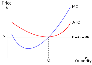
• In the short-run, perfectly competitive markets are not necessarily productively efficient, as output will not always occur where marginal cost is equal to average cost (MC = AC). However, in the long-run, productive efficiency occurs as new firms enter the industry. Competition reduces price and cost to the minimum of the long run average costs. At this point, price equals both the marginal cost and the average total cost for each good (P = MC = AC).

The theory of perfect competition has its roots in late-19th century economic thought. Léon Walras^[2] gave the first rigorous definition of perfect competition and derived some of its main results. In the 1950s, the theory was further formalized by Kenneth Arrow and Gérard Debreu.^[3]

Imperfect competition was a theory created to explain the more realistic kind of market interaction that lies in between perfect competition and a monopoly. Edward Chamberlin wrote "Monopolistic Competition" in 1933 as "a challenge to the traditional viewpoint that competition and monopolies are alternatives and that individual prices are to be explained in either terms of one or the other" (Dewey,88.) In this book, and for much of his career, he "analyzed firms that do not produce identical goods, but goods that are close substitutes for one another" (Sandmo,300.)

Another key player in understanding imperfect competition is Joan Robinson, who published her book "The Economics of Perfect Competition" the same year Chamberlain published his. While Chamberlain focused much of his work on product development, Robinson focused heavily on price formation and discrimination (Sandmo,303.) The act of price discrimination under imperfect competition implies that the seller would sell their goods at different prices depending on the characteristic of the buyer to increase revenue (Robinson,204.) Joan Robinson and Edward Chamberlain came to many of the same conclusions regarding imperfect competition while still adding a bit of their twist to the theory. Despite their similarities or disagreements about who discovered the idea, both were extremely helpful in allowing firms to understand better how to center their goods around the wants of the consumer to achieve the highest amount of revenue possible.

Real markets are never perfect. Those economists who believe in perfect competition as a useful approximation to real markets may classify those as ranging from close-to-perfect to very imperfect. The real estate market is an example of a very imperfect market. In such markets, the theory of the second best proves that if one optimality condition in an economic model cannot be satisfied, it is possible that the next-best solution involves changing other variables away from the values that would otherwise be optimal.

Idealizing conditions of perfect competition

There is a set of market conditions which are assumed to prevail in the discussion of what perfect competition might be if it were theoretically possible to ever obtain such perfect market conditions. These conditions include:

• A large number of buyers and sellers – A large number of consumers with the willingness and ability to buy the product at a certain price, and a large number of producers with the willingness and ability to supply the product at a certain price. As a result, individuals are unable to influence prices more than a little.
• Anti-competitive regulation: It is assumed that a market of perfect competition shall provide the regulations and protections implicit in the control of and elimination of anti-competitive activity in the market place.
• Every participant is a price taker: No participant with market power to set prices.
• Homogeneous products: The products are perfect substitutes for each other (i.e., the qualities and characteristics of a market good or service do not vary between different suppliers). There are many instances in which there exist "similar" products that are close substitutes (such as butter and margarine), which are relatively easily interchangeable, so that a rise in the price of one good will cause a significant shift to the consumption of the close substitute. If the cost of changing a firm's manufacturing process to produce the substitute is also relatively "immaterial" in relationship to the firm's overall profit and cost, this is sufficient to ensure that an economic situation isn't significantly different from a perfectly competitive economic market.
• Rational buyers: Buyers make all trades that increase their economic utility and make no trades that do not.
• No barriers to entry or exit: This implies that both entry and exit must be perfectly free of sunk costs.
• No externalities: Costs or benefits of an activity do not affect third parties. This criterion also excludes any government intervention.
• Non-increasing returns to scale and no network effects: The lack of economies of scale or network effects ensures that there will always be a sufficient number of firms in the industry.
• Perfect factor mobility: In the long run factors of production are perfectly mobile, allowing free long term adjustments to changing market conditions. This allows workers to freely move between firms.
• Perfect information: All consumers and producers know all prices of products and utilities they would get from owning each product. This prevents firms from obtaining any information which would give them a competitive edge.
• Profit maximization of sellers: Firms sell where the most profit is generated, where marginal costs meet marginal revenue.
• Well defined property rights: These determine what may be sold, as well as what rights are conferred on the buyer.
• Zero transaction costs: Buyers and sellers do not incur costs in making an exchange of goods.

Normal profit

In a perfect market the sellers operate at zero economic surplus: sellers make a level of return on investment known as normal profits.

Normal profit is a component of (implicit) costs and not a component of business profit at all. It represents all the opportunity cost, as the time that the owner spends running the firm could be spent on running a different firm. The enterprise component of normal profit is thus the profit that a business owner considers necessary to make running the business worth while: that is, it is comparable to the next best amount the entrepreneur could earn doing another job. Particularly if enterprise is not included as a factor of production, it can also be viewed a return to capital for investors including the entrepreneur, equivalent to the return the capital owner could have expected (in a safe investment), plus compensation for risk. In other words, the cost of normal profit varies both within and across industries; it is commensurate with the riskiness associated with each type of investment, as per the risk–return spectrum.

In circumstances of perfect competition, only normal profits arise when the long run economic equilibrium is reached; there is no incentive for firms to either enter or leave the industry.

In competitive and contestable markets

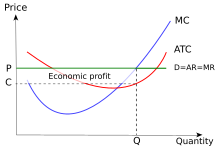
Only in the short run can a firm in a perfectly competitive market make an economic profit.

Economic profit does not occur in perfect competition in long run equilibrium; if it did, there would be an incentive for new firms to enter the industry, aided by a lack of barriers to entry until there was no longer any economic profit. As new firms enter the industry, they increase the supply of the product available in the market, and these new firms are forced to charge a lower price to entice consumers to buy the additional supply these new firms are supplying as the firms all compete for customers (See "Persistence" in the Monopoly Profit discussion). Incumbent firms within the industry face losing their existing customers to the new firms entering the industry, and are therefore forced to lower their prices to match the lower prices set by the new firms. New firms will continue to enter the industry until the price of the product is lowered to the point that it is the same as the average cost of producing the product, and all of the economic profit disappears. When this happens, economic agents outside of the industry find no advantage to forming new firms that enter into the industry, the supply of the product stops increasing, and the price charged for the product stabilizes, settling into an equilibrium.

The same is likewise true of the long run equilibria of monopolistically competitive industries and, more generally, any market which is held to be contestable. Normally, a firm that introduces a differentiated product can initially secure a temporary market power for a short while (See "Persistence" in Monopoly Profit). At this stage, the initial price the consumer must pay for the product is high, and the demand for, as well as the availability of the product in the market, will be limited. In the long run, however, when the profitability of the product is well established, and because there are few barriers to entry, the number of firms that produce this product will increase until the available supply of the product eventually becomes relatively large, the price of the product shrinks down to the level of the average cost of producing the product. When this finally occurs, all monopoly profit associated with producing and selling the product disappears, and the initial monopoly turns into a competitive industry. In the case of contestable markets, the cycle is often ended with the departure of the former "hit and run" entrants to the market, returning the industry to its previous state, just with a lower price and no economic profit for the incumbent firms.

Profit can, however, occur in competitive and contestable markets in the short run, as firms jostle for market position. Once risk is accounted for, long-lasting economic profit in a competitive market is thus viewed as the result of constant cost-cutting and performance improvement ahead of industry competitors, allowing costs to be below the market-set price.

In non competitive markets

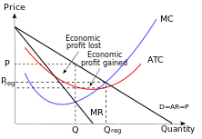
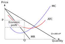
A monopolist can set a price in excess of costs, making an economic profit. The above diagram shows a monopolist (only one firm in the market) that obtains a (monopoly) economic profit. An oligopoly usually has economic profit also, but operates in a market with more than just one firm (they must share available demand at the market price).

Economic profit is, however, much more prevalent in uncompetitive markets such as in a perfect monopoly or oligopoly situation. In these scenarios, individual firms have some element of market power: Though monopolists are constrained by consumer demand, they are not price takers, but instead either price-setters or quantity setters. This allows the firm to set a price that is higher than that which would be found in a similar but more competitive industry, allowing them economic profit in both the long and short run.

The existence of economic profits depends on the prevalence of barriers to entry: these stop other firms from entering into the industry and sapping away profits, as they would in a more competitive market. In cases where barriers are present, but more than one firm, firms can collude to limit production, thereby restricting supply in order to ensure that the price of the product remains high enough for all firms in the industry to achieve an economic profit.

However, some economists, for instance Steve Keen, a professor at the University of Western Sydney, argue that even an infinitesimal amount of market power can allow a firm to produce a profit and that the absence of economic profit in an industry, or even merely that some production occurs at a loss, in and of itself constitutes a barrier to entry.

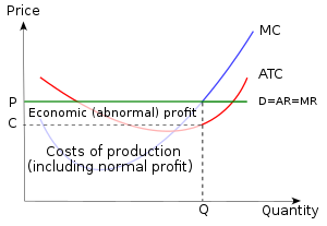
In a single-goods case, a positive economic profit happens when the firm's average cost is less than the price of the product or service at the profit-maximizing output. The economic profit is equal to the quantity of output multiplied by the difference between the average cost and the price.

Government intervention

Often, governments will try to intervene in uncompetitive markets to make them more competitive. Antitrust (US) or competition (elsewhere) laws were created to prevent powerful firms from using their economic power to artificially create the barriers to entry they need to protect their economic profits. This includes the use of predatory pricing toward smaller competitors. For example, in the United States, Microsoft Corporation was initially convicted of breaking Anti-Trust Law and engaging in anti-competitive behavior in order to form one such barrier in United States v. Microsoft; after a successful appeal on technical grounds, Microsoft agreed to a settlement with the Department of Justice in which they were faced with stringent oversight procedures and explicit requirements designed to prevent this predatory behaviour. With lower barriers, new firms can enter the market again, making the long run equilibrium more like that of a competitive industry, with no economic profit for firms.

In a regulated industry, the government examines firms' marginal cost structure and allows them to charge a price that is no greater than this marginal cost. This does not necessarily ensure zero Economic profit for the firm, but eliminates a "Pure Monopoly" Profit.

If a government feels it is impractical to have a competitive market – such as in the case of a natural monopoly – it will sometimes try to regulate the existing uncompetitive market by controlling the price firms charge for their product. For example, the old AT&T (regulated) monopoly, which existed before the courts ordered its breakup, had to get government approval to raise its prices. The government examined the monopoly's costs to determine whether the monopoly should be able raise its price, and could reject the monopoly's application for a higher price if the cost did not justify it. Although a regulated firm will not have an economic profit as large as it would in an unregulated situation, it can still make profits well above a competitive firm in a truly competitive market.

Results

In the short run, it is possible for an individual firm to make an economic profit. This situation is shown in this diagram, as the price or average revenue, denoted by P, is above the average cost denoted by C .

 

However, in the long run, economic profit cannot be sustained. The arrival of new firms or expansion of existing firms (if returns to scale are constant) in the market causes the (horizontal) demand curve of each individual firm to shift downward, bringing down at the same time the price, the average revenue and marginal revenue curve. The outcome is that, in the long run, the firm will make only normal profit (zero economic profit). Its horizontal demand curve will touch its average total cost curve at its lowest point. (See cost curve.)

In a perfectly competitive market, the demand curve facing a firm is perfectly elastic.

As mentioned above, the perfect competition model, if interpreted as applying also to short-period or very-short-period behaviour, is approximated only by markets of homogeneous products produced and purchased by very many sellers and buyers, usually organized markets for agricultural products or raw materials. In real-world markets, assumptions such as perfect information cannot be verified and are only approximated in organized double-auction markets where most agents wait and observe the behaviour of prices before deciding to exchange (but in the long-period interpretation perfect information is not necessary, the analysis only aims at determining the average around which market prices gravitate, and for gravitation to operate one does not need perfect information).

In the absence of externalities and public goods, perfectly competitive equilibria are Pareto-efficient, i.e. no improvement in the utility of a consumer is possible without a worsening of the utility of some other consumer. This is called the First Theorem of Welfare Economics. The basic reason is that no productive factor with a non-zero marginal product is left unutilized, and the units of each factor are so allocated as to yield the same indirect marginal utility in all uses, a basic efficiency condition (if this indirect marginal utility were higher in one use than in other ones, a Pareto improvement could be achieved by transferring a small amount of the factor to the use where it yields a higher marginal utility).

A simple proof assuming differentiable utility functions and production functions is the following. Let w_j be the 'price' (the rental) of a certain factor j, let MP_j1 and MP_j2 be its marginal product in the production of goods 1 and 2, and let p₁ and p₂ be these goods' prices. In equilibrium these prices must equal the respective marginal costs MC₁ and MC₂; remember that marginal cost equals factor 'price' divided by factor marginal productivity (because increasing the production of good by one very small unit through an increase of the employment of factor j requires increasing the factor employment by 1/MP_ji and thus increasing the cost by w_j/MP_ji, and through the condition of cost minimization that marginal products must be proportional to factor 'prices' it can be shown that the cost increase is the same if the output increase is obtained by optimally varying all factors). Optimal factor employment by a price-taking firm requires equality of factor rental and factor marginal revenue product, w_j=p_iMP_ji, so we obtain p₁=MC₁=w_j/MP_j1, p₂=MC_j2=w_j/MP_j2.

Now choose any consumer purchasing both goods, and measure his utility in such units that in equilibrium his marginal utility of money (the increase in utility due to the last unit of money spent on each good), MU₁/p₁=MU₂/p₂, is 1. Then p₁=MU₁, p₂=MU₂. The indirect marginal utility of the factor is the increase in the utility of our consumer achieved by an increase in the employment of the factor by one (very small) unit; this increase in utility through allocating the small increase in factor utilization to good 1 is MP_j1MU₁=MP_j1p₁=w_j, and through allocating it to good 2 it is MP_j2MU₂=MP_j2p₂=w_j again. With our choice of units the marginal utility of the amount of the factor consumed directly by the optimizing consumer is again w, so the amount supplied of the factor too satisfies the condition of optimal allocation.

Monopoly violates this optimal allocation condition, because in a monopolized industry market price is above marginal cost, and this means that factors are underutilized in the monopolized industry, they have a higher indirect marginal utility than in their uses in competitive industries. Of course, this theorem is considered irrelevant by economists who do not believe that general equilibrium theory correctly predicts the functioning of market economies; but it is given great importance by neoclassical economists and it is the theoretical reason given by them for combating monopolies and for antitrust legislation.

Profit

In contrast to a monopoly or oligopoly, in perfect competition it is impossible for a firm to earn economic profit in the long run, which is to say that a firm cannot make any more money than is necessary to cover its economic costs. In order not to misinterpret this zero-long-run-profits thesis, it must be remembered that the term 'profit' is used in different ways:

• Neoclassical theory defines profit as what is left of revenue after all costs have been subtracted; including normal interest on capital plus the normal excess over it required to cover risk, and normal salary for managerial activity. This means that profit is calculated after the actors are compensated for their opportunity costs.
• Classical economists on the contrary define profit as what is left after subtracting costs except interest and risk coverage. Thus, the classical approach does not account for opportunity costs.

Thus, if one leaves aside risk coverage for simplicity, the neoclassical zero-long-run-profit thesis would be re-expressed in classical parlance as profits coinciding with interest in the long period (i.e. the rate of profit tending to coincide with the rate of interest). Profits in the classical meaning do not necessarily disappear in the long period but tend to normal profit. With this terminology, if a firm is earning abnormal profit in the short term, this will act as a trigger for other firms to enter the market. As other firms enter the market, the market supply curve will shift out, causing prices to fall. Existing firms will react to this lower price by adjusting their capital stock downward. This adjustment will cause their marginal cost to shift to the left causing the market supply curve to shift inward. However, the net effect of entry by new firms and adjustment by existing firms will be to shift the supply curve outward. The market price will be driven down until all firms are earning normal profit only.

It is important to note that perfect competition is a sufficient condition for allocative and productive efficiency, but it is not a necessary condition. Laboratory experiments in which participants have significant price setting power and little or no information about their counterparts consistently produce efficient results given the proper trading institutions.

Shutdown point

In the short run, a firm operating at a loss [R < TC (revenue less than total cost) or P < ATC (price less than unit cost)] must decide whether to continue to operate or temporarily shut down. The shutdown rule states "in the short run a firm should continue to operate if price exceeds average variable costs". Restated, the rule is that for a firm to continue producing in the short run it must earn sufficient revenue to cover its variable costs. The rationale for the rule is straightforward: By shutting down a firm avoids all variable costs. However, the firm must still pay fixed costs. Because fixed costs must be paid regardless of whether a firm operates they should not be considered in deciding whether to produce or shut down. Thus in determining whether to shut down a firm should compare total revenue to total variable costs (VC) rather than total costs (FC + VC). If the revenue the firm is receiving is greater than its total variable cost (R > VC), then the firm is covering all variable costs and there is additional revenue ("contribution"), which can be applied to fixed costs. (The size of the fixed costs is irrelevant as it is a sunk cost. The same consideration is used whether fixed costs are one dollar or one million dollars.) On the other hand, if VC > R then the firm is not covering its production costs and it should immediately shut down. The rule is conventionally stated in terms of price (average revenue) and average variable costs. The rules are equivalent (if one divides both sides of inequality TR > TVC by Q gives P > AVC). If the firm decides to operate, the firm will continue to produce where marginal revenue equals marginal costs because these conditions insure not only profit maximization (loss minimization) but also maximum contribution.

Another way to state the rule is that a firm should compare the profits from operating to those realized if it shut down and select the option that produces the greater profit. A firm that is shut down is generating zero revenue and incurring no variable costs. However, the firm still has to pay fixed cost. So the firm's profit equals fixed costs or −FC. An operating firm is generating revenue, incurring variable costs and paying fixed costs. The operating firm's profit is R − VC − FC. The firm should continue to operate if R − VC − FC ≥ −FC, which simplified is R ≥ VC. The difference between revenue, R, and variable costs, VC, is the contribution to fixed costs and any contribution is better than none. Thus, if R ≥ VC then firm should operate. If R < VC the firm should shut down.

A decision to shut down means that the firm is temporarily suspending production. It does not mean that the firm is going out of business (exiting the industry). If market conditions improve, and prices increase, the firm can resume production. Shutting down is a short-run decision. A firm that has shut down is not producing. The firm still retains its capital assets; however, the firm cannot leave the industry or avoid its fixed costs in the short run. Exit is a long-term decision. A firm that has exited an industry has avoided all commitments and freed all capital for use in more profitable enterprises.

However, a firm cannot continue to incur losses indefinitely. In the long run, the firm will have to earn sufficient revenue to cover all its expenses and must decide whether to continue in business or to leave the industry and pursue profits elsewhere. The long-run decision is based on the relationship of the price and long-run average costs. If P ≥ AC then the firm will not exit the industry. If P < AC, then the firm will exit the industry. These comparisons will be made after the firm has made the necessary and feasible long-term adjustments. In the long run a firm operates where marginal revenue equals long-run marginal costs.

Short-run supply curve

The short-run (SR) supply curve for a perfectly competitive firm is the marginal cost (MC) curve at and above the shutdown point. Portions of the marginal cost curve below the shutdown point are not part of the SR supply curve because the firm is not producing any positive quantity in that range. Technically the SR supply curve is a discontinuous function composed of the segment of the MC curve at and above minimum of the average variable cost curve and a segment that runs on the vertical axis from the origin to but not including a point at the height of the minimum average variable cost.

Criticisms

The use of the assumption of perfect competition as the foundation of price theory for product markets is often criticized as representing all agents as passive, thus removing the active attempts to increase one's welfare or profits by price undercutting, product design, advertising, innovation, activities that – the critics argue – characterize most industries and markets. These criticisms point to the frequent lack of realism of the assumptions of product homogeneity and impossibility to differentiate it, but apart from this, the accusation of passivity appears correct only for short-period or very-short-period analyses, in long-period analyses the inability of price to diverge from the natural or long-period price is due to active reactions of entry or exit.

Some economists have a different kind of criticism concerning perfect competition model. They are not criticizing the price taker assumption because it makes economic agents too "passive", but because it then raises the question of who sets the prices. Indeed, if everyone is price taker, there is the need for a benevolent planner who gives and sets the prices, in other word, there is a need for a "price maker". Therefore, it makes the perfect competition model appropriate not to describe a decentralized "market" economy but a centralized one. This in turn means that such kind of model has more to do with communism than capitalism.

Another frequent criticism is that it is often not true that in the short run differences between supply and demand cause changes in price; especially in manufacturing, the more common behaviour is alteration of production without nearly any alteration of price.

The critics of the assumption of perfect competition in product markets seldom question the basic neoclassical view of the working of market economies for this reason. The Austrian School insists strongly on this criticism, and yet the neoclassical view of the working of market economies as fundamentally efficient, reflecting consumer choices and assigning to each agent his contribution to social welfare, is esteemed to be fundamentally correct. Some non-neoclassical schools, like Post-Keynesians, reject the neoclassical approach to value and distribution, but not because of their rejection of perfect competition as a reasonable approximation to the working of most product markets; the reasons for rejection of the neoclassical 'vision' are different views of the determinants of income distribution and of aggregated demand.

In particular, the rejection of perfect competition does not generally entail the rejection of free competition as characterizing most product markets; indeed it has been argued that competition is stronger nowadays than in 19th century capitalism, owing to the increasing capacity of big conglomerate firms to enter any industry: therefore the classical idea of a tendency toward a uniform rate of return on investment in all industries owing to free entry is even more valid today; and the reason why General Motors, Exxon or Nestlé do not enter the computers or pharmaceutical industries is not insurmountable barriers to entry but rather that the rate of return in the latter industries is already sufficiently in line with the average rate of return elsewhere as not to justify entry. On this few economists, it would seem, would disagree, even among the neoclassical ones. Thus when the issue is normal, or long-period, product prices, differences on the validity of the perfect competition assumption do not appear to imply important differences on the existence or not of a tendency of rates of return toward uniformity as long as entry is possible, and what is found fundamentally lacking in the perfect competition model is the absence of marketing expenses and innovation as causes of costs that do enter normal average cost.

The issue is different with respect to factor markets. Here the acceptance or denial of perfect competition in labour markets does make a big difference to the view of the working of market economies. One must distinguish neoclassical from non-neoclassical economists. For the former, absence of perfect competition in labour markets, e.g. due to the existence of trade unions, impedes the smooth working of competition, which if left free to operate would cause a decrease of wages as long as there were unemployment, and would finally ensure the full employment of labour: labour unemployment is due to absence of perfect competition in labour markets. Most non-neoclassical economists deny that a full flexibility of wages would ensure the full employment of labour and find a stickiness of wages an indispensable component of a market economy, without which the economy would lack the regularity and persistence indispensable to its smooth working. This was, for example, John Maynard Keynes's opinion.

Particularly radical is the view of the Sraffian school on this issue: the labour demand curve cannot be determined hence a level of wages ensuring the equality between supply and demand for labour does not exist, and economics should resume the viewpoint of the classical economists, according to whom competition in labour markets does not and cannot mean indefinite price flexibility as long as supply and demand are unequal, it only means a tendency to equality of wages for similar work, but the level of wages is necessarily determined by complex sociopolitical elements; custom, feelings of justice, informal allegiances to classes, as well as overt coalitions such as trade unions, far from being impediments to a smooth working of labour markets that would be able to determine wages even without these elements, are on the contrary indispensable because without them there would be no way to determine wages.

Equilibrium in perfect competition

Equilibrium in perfect competition is the point where market demands will be equal to market supply. A firm's price will be determined at this point. In the short run, equilibrium will be affected by demand. In the long run, both demand and supply of a product will affect the equilibrium in perfect competition. A firm will receive only normal profit in the long run at the equilibrium point.

As it is well known, requirements for firm's cost-curve under perfect competition is for the slope to move upwards after a certain amount is produced. This amount is small enough to leave a sufficiently large number of firms in the field (for any given total outputs in the industry) for the conditions of perfect competition to be preserved. For the short-run, the supply of some factors are assumed to be fixed and as the price of the other factors are given, costs per unit must necessarily rise after a certain point. From a theoretical point of view, given the assumptions that there will be a tendency for continuous growth in size for firms, long-period static equilibrium alongside perfect competition may be incompatible.

Economic equilibrium

From Wikipedia, the free encyclopedia

https://en.wikipedia.org/wiki/Economic_equilibrium 

 

Economic equilibrium
A solution concept in game theory
Relationship
Subset of	Equilibrium, Free market
Superset of	Competitive equilibrium, Nash equilibrium, Intertemporal equilibrium, Recursive competitive equilibrium
Significance

Used for	mostly Perfect competition, but also some Imperfect competition

In economics, economic equilibrium is a situation in which economic forces such as supply and demand are balanced and in the absence of external influences the (equilibrium) values of economic variables will not change. For example, in the standard text perfect competition, equilibrium occurs at the point at which quantity demanded and quantity supplied are equal.

Market equilibrium in this case is a condition where a market price is established through competition such that the amount of goods or services sought by buyers is equal to the amount of goods or services produced by sellers. This price is often called the competitive price or market clearing price and will tend not to change unless demand or supply changes, and quantity is called the "competitive quantity" or market clearing quantity. But the concept of equilibrium in economics also applies to imperfectly competitive markets, where it takes the form of a Nash equilibrium.

Understanding economic equilibrium

An economic equilibrium is a situation when the economic agent cannot change the situation by adopting any strategy. To fully grasp the concept of economic equilibrium, it must be highlighted that it has been borrowed from the physical sciences. Take a system where physical forces are balanced for instance.This economically interpreted means no further change ensues.

Properties of equilibrium

Three basic properties of equilibrium in general have been proposed by Huw Dixon. These are:

Equilibrium property P1: The behavior of agents is consistent.

Equilibrium property P2: No agent has an incentive to change its behavior.

Equilibrium property P3: Equilibrium is the outcome of some dynamic process (stability).

Example: competitive equilibrium

Competitive Equilibrium: Price equates supply and demand.

• P – price
• Q – quantity demanded and supplied
• S – supply curve
• D – demand curve
• P₀ – equilibrium price
• A – excess demand – when P<P₀
• B – excess supply – when P>P₀

In a competitive equilibrium, supply equals demand. Property P1 is satisfied, because at the equilibrium price the amount supplied is equal to the amount demanded. Property P2 is also satisfied. Demand is chosen to maximize utility given the market price: no one on the demand side has any incentive to demand more or less at the prevailing price. Likewise supply is determined by firms maximizing their profits at the market price: no firm will want to supply any more or less at the equilibrium price. Hence, agents on neither the demand side nor the supply side will have any incentive to alter their actions.

To see whether Property P3 is satisfied, consider what happens when the price is above the equilibrium. In this case there is an excess supply, with the quantity supplied exceeding that demanded. This will tend to put downward pressure on the price to make it return to equilibrium. Likewise where the price is below the equilibrium point there is a shortage in supply leading to an increase in prices back to equilibrium. Not all equilibria are "stable" in the sense of equilibrium property P3. It is possible to have competitive equilibria that are unstable. However, if an equilibrium is unstable, it raises the question of reaching it. Even if it satisfies properties P1 and P2, the absence of P3 means that the market can only be in the unstable equilibrium if it starts off there.

In most simple microeconomic stories of supply and demand a static equilibrium is observed in a market; however, economic equilibrium can be also dynamic. Equilibrium may also be economy-wide or general, as opposed to the partial equilibrium of a single market. Equilibrium can change if there is a change in demand or supply conditions. For example, an increase in supply will disrupt the equilibrium, leading to lower prices. Eventually, a new equilibrium will be attained in most markets. Then, there will be no change in price or the amount of output bought and sold — until there is an exogenous shift in supply or demand (such as changes in technology or tastes). That is, there are no endogenous forces leading to the price or the quantity.

Example: monopolist equilibrium

In a monopoly, marginal revenue (MR) equals marginal cost (MC). The equilibrium quantity is obtained from where MR and MC intersect and the equilibrium price can be found on the demand curve where MR = MC. Property P1 is not satisfied because the amount demand and the amount supplied at the equilibrium price are not equal. Property P2 is not satisfied. Because the monopolist's profit-maximizing quantity is different from the socially-maximizing quantity, consumer's have an incentive to demand more at the equilibrium price. However, at the market price, monopolists maximize their profits so they have no incentive to change their price. Therefore, agents on the demand side have an incentive to alter their actions while the agents on the supply side do not have any incentive to alter their actions.

In order to determine if Property P3 is satisfied, the same situations used to determine P3 in a competitive equilibrium can be used. When there is an excess in supply, monopolists will realize that the equilibrium is not at the profit-maximizing quantity and will put upward pressure on the price to make it return to equilibrium. This is the same case when the price is above the equilibrium and the shortage in supply leads the monopolist to decrease the supply to return to the profit-maximizing quantity. Therefore the equilibrium is the result of stability.

Example: Nash equilibrium

Further information: Nash equilibrium and Cournot model

Equilibrium quantities as a solution to two reaction functions in Cournot duopoly. Firm 1's reaction function q1=R1(q2) gives its optimal output q1 to a given output q2 of firm 2. Likewise, firm 2's reaction function q2=R2(q1). The Cournot-Nash equilibrium occurs where the two reaction functions intersect and both firms are choosing the optimal output given the output of the other firm.

The Nash equilibrium is widely used in economics as the main alternative to competitive equilibrium. It is used whenever there is a strategic element to the behavior of agents and the "price taking" assumption of competitive equilibrium is inappropriate. The first use of the Nash equilibrium was in the Cournot duopoly as developed by Antoine Augustin Cournot in his 1838 book. Both firms produce a homogenous product: given the total amount supplied by the two firms, the (single) industry price is determined using the demand curve. This determines the revenues of each firm (the industry price times the quantity supplied by the firm). The profit of each firm is then this revenue minus the cost of producing the output. Clearly, there is a strategic interdependence between the two firms. If one firm varies its output, this will in turn affect the market price and so the revenue and profits of the other firm. We can define the payoff function which gives the profit of each firm as a function of the two outputs chosen by the firms. Cournot assumed that each firm chooses its own output to maximize its profits given the output of the other firm. The Nash equilibrium occurs when both firms are producing the outputs which maximize their own profit given the output of the other firm.

In terms of the equilibrium properties, we can see that P2 is satisfied: in a Nash equilibrium, neither firm has an incentive to deviate from the Nash equilibrium given the output of the other firm. P1 is satisfied since the payoff function ensures that the market price is consistent with the outputs supplied and that each firms profits equal revenue minus cost at this output.

Is the equilibrium stable as required by P3? Cournot himself argued that it was stable using the stability concept implied by best response dynamics. The reaction function for each firm gives the output which maximizes profits (best response) in terms of output for a firm in terms of a given output of the other firm. In the standard Cournot model this is downward sloping: if the other firm produces a higher output, the best response involves producing less. Best response dynamics involves firms starting from some arbitrary position and then adjusting output to their best-response to the previous output of the other firm. So long as the reaction functions have a slope of less than -1, this will converge to the Nash equilibrium. However, this stability story is open to much criticism. As Dixon argues: "The crucial weakness is that, at each step, the firms behave myopically: they choose their output to maximize their current profits given the output of the other firm, but ignore the fact that the process specifies that the other firm will adjust its output...". There are other concepts of stability that have been put forward for the Nash equilibrium, evolutionary stability for example.

Example: Walrasian equilibrium in a Power economy

Walrasian Equilibrium Prices

A fictional auctioneer calls out prices. Consumers and firms report honestly their demands and supplies.

When Net Demand = [Demand - Supply] is zero, the auctioneer's job is done. The prices are market clearing prices.

Special case: An island economy.

Supply

Consumers a and b survive by consuming coconuts that fall from the palm trees, x, and crayfish, y, trapped in the lagoon. This yields 1 basketful per day of each commodity.

Only the price ratio p = p₁/p₂ matters so the auctioneer only has to call out one price.

There is one daily basketful of each commodity. Therefore the supply is 1=(1,1).

Demand

The marginal rates of rates of substitution in Power σ economy are MRS(a)=(Ax(a)/y(a))^1/σ and MRS(b)=(Bx(b)/y(b))^1/σ

(Pareto) Efficient Allocations

The marginal rates of substitution are the same for an efficient allocation. So (Ax(a)/y(a))^1/σ = (Bx(b)/y(b))^1/σ.

Therefore, for all Powers the condition for efficiency is Ax(a)/y(a) and MRS(b)=Bx(b)/y(b). This yields the first big result.

Proposition: Efficiency in a Power Economy

If an allocation is (in)-efficient in any power economy, then it is (in)-efficient in all power economies.

Consumer Choice

A consumer's choice is an allocation for which the consumer's marginal willingness to trade is equal to the price ratio.

Market Clearing equations in a power σ economy

The marginal rates of substitution must be the same. Therefore, p =(Ax(a)/y(a)^1/σ =(Bx(b)/y(b))^1/σ. IT follows that

μ = p^σ = Ax/y and p = B(1-x)/(1-y))

Key observation: The two market clearing equations are two equations for the three variables, x, y and σ. Therefore, any one of the variables can be eliminated.

The result is three equations for two variables.

Let the difference in the parameters be D. Let the multiplication of the parameters be M

Demand equations in a Power Economy

y(p) = (p^1/σ - B)/(AD²) and x(p)= (1-(1/p^1/σ))(M/D). where D=A-B and M=AB

Demand Price Equations in a power economy:

p^1/σ = B - Dy and p^1/σ = 1/(1-x(D/M))

The characteristic equation E(z)=z₁z₂ in a power economy

This is a rectangular hyperbola

Mutliplying the two demand price equations. The efficient allocations are on a level set of the following rectangular hyperbola

E(x,y) = (x-AD)(y+B/D) = K, where D=A-B and M=AB

If consumer a is allocated everything, this is efficient allocation. Any reallocation makes consumer a worse off. Therefore K=-AB.

Market clearing prices

Most economists, for example Paul Samuelson, caution against attaching a normative meaning (value judgement) to the equilibrium price. For example, food markets may be in equilibrium at the same time that people are starving (because they cannot afford to pay the high equilibrium price). Indeed, this occurred during the Great Famine in Ireland in 1845–52, where food was exported though people were starving, due to the greater profits in selling to the English – the equilibrium price of the Irish-British market for potatoes was above the price that Irish farmers could afford, and thus (among other reasons) they starved.

Interpretations

In most interpretations, classical economists such as Adam Smith maintained that the free market would tend towards economic equilibrium through the price mechanism. That is, any excess supply (market surplus or glut) would lead to price cuts, which decrease the quantity supplied (by reducing the incentive to produce and sell the product) and increase the quantity demanded (by offering consumers bargains), automatically abolishing the glut. Similarly, in an unfettered market, any excess demand (or shortage) would lead to price increases, reducing the quantity demanded (as customers are priced out of the market) and increasing in the quantity supplied (as the incentive to produce and sell a product rises). As before, the disequilibrium (here, the shortage) disappears. This automatic abolition of non-market-clearing situations distinguishes markets from central planning schemes, which often have a difficult time getting prices right and suffer from persistent shortages of goods and services.

This view came under attack from at least two viewpoints. Modern mainstream economics points to cases where equilibrium does not correspond to market clearing (but instead to unemployment), as with the efficiency wage hypothesis in labor economics. In some ways parallel is the phenomenon of credit rationing, in which banks hold interest rates low to create an excess demand for loans, so they can pick and choose whom to lend to. Further, economic equilibrium can correspond with monopoly, where the monopolistic firm maintains an artificial shortage to prop up prices and to maximize profits. Finally, Keynesian macroeconomics points to underemployment equilibrium, where a surplus of labor (i.e., cyclical unemployment) co-exists for a long time with a shortage of aggregate demand.

Solving for the competitive equilibrium price

To find the equilibrium price, one must either plot the supply and demand curves, or solve for the expressions for supply and demand being equal.

An example may be:

${\displaystyle \begin{array}{rl}{Q}_s& =125+1.5\cdot P\\ Q_d& =189-2.25\cdot P\\ \\ Q_s& =Q_d\\ \\ 125+1.5\cdot P& =189-2.25\cdot P\\ (1.5+2.25)\cdot P& =(189-125)\\ P& =\frac{189-125}{1.5+2.25}\\ P& =\frac{64}{3.75}\\ P& =17.067\end{array}}$

In the diagram, depicting simple set of supply and demand curves, the quantity demanded and supplied at price P are equal.

At any price above P supply exceeds demand, while at a price below P the quantity demanded exceeds that supplied. In other words, prices where demand and supply are out of balance are termed points of disequilibrium, creating shortages and oversupply. Changes in the conditions of demand or supply will shift the demand or supply curves. This will cause changes in the equilibrium price and quantity in the market.

Consider the following demand and supply schedule:

Price ($)	Demand	Supply
8.00	6,000	18,000
7.00	8,000	16,000
6.00	10,000	14,000
5.00	12,000	12,000
4.00	14,000	10,000
3.00	16,000	8,000
2.00	18,000	6,000
1.00	20,000	4,000

• The equilibrium price in the market is $5.00 where demand and supply are equal at 12,000 units
• If the current market price was $3.00 – there would be excess demand for 8,000 units, creating a shortage.
• If the current market price was $8.00 – there would be excess supply of 12,000 units.

When there is a shortage in the market we see that, to correct this disequilibrium, the price of the good will be increased back to a price of $5.00, thus lessening the quantity demanded and increasing the quantity supplied thus that the market is in balance.

When there is an oversupply of a good, such as when price is above $6.00, then we see that producers will decrease the price to increase the quantity demanded for the good, thus eliminating the excess and taking the market back to equilibrium.

Influences changing price

A change in equilibrium price may occur through a change in either the supply or demand schedules. For instance, starting from the above supply-demand configuration, an increased level of disposable income may produce a new demand schedule, such as the following:

Price ($)	Demand	Supply
8.00	10,000	18,000
7.00	12,000	16,000
6.00	14,000	14,000
5.00	16,000	12,000
4.00	18,000	10,000
3.00	20,000	8,000
2.00	22,000	6,000
1.00	24,000	4,000

Here we see that an increase in disposable income would increase the quantity demanded of the good by 2,000 units at each price. This increase in demand would have the effect of shifting the demand curve rightward. The result is a change in the price at which quantity supplied equals quantity demanded. In this case we see that the two now equal each other at an increased price of $6.00. Note that a decrease in disposable income would have the exact opposite effect on the market equilibrium.

We will also see similar behaviour in price when there is a change in the supply schedule, occurring through technological changes, or through changes in business costs. An increase in technological usage or know-how or a decrease in costs would have the effect of increasing the quantity supplied at each price, thus reducing the equilibrium price. On the other hand, a decrease in technology or increase in business costs will decrease the quantity supplied at each price, thus increasing equilibrium price.

The process of comparing two static equilibria to each other, as in the above example, is known as comparative statics. For example, since a rise in consumers' income leads to a higher price (and a decline in consumers' income leads to a fall in the price — in each case the two things change in the same direction), we say that the comparative static effect of consumer income on the price is positive. This is another way of saying that the total derivative of price with respect to consumer income is greater than zero.

Dynamic equilibrium

Whereas in a static equilibrium all quantities have unchanging values, in a dynamic equilibrium various quantities may all be growing at the same rate, leaving their ratios unchanging. For example, in the neoclassical growth model, the working population is growing at a rate which is exogenous (determined outside the model, by non-economic forces). In dynamic equilibrium, output and the physical capital stock also grow at that same rate, with output per worker and the capital stock per worker unchanging. Similarly, in models of inflation a dynamic equilibrium would involve the price level, the nominal money supply, nominal wage rates, and all other nominal values growing at a single common rate, while all real values are unchanging, as is the inflation rate.

The process of comparing two dynamic equilibria to each other is known as comparative dynamics. For example, in the neoclassical growth model, starting from one dynamic equilibrium based in part on one particular saving rate, a permanent increase in the saving rate leads to a new dynamic equilibrium in which there are permanently higher capital per worker and productivity per worker, but an unchanged growth rate of output; so it is said that in this model the comparative dynamic effect of the saving rate on capital per worker is positive but the comparative dynamic effect of the saving rate on the output growth rate is zero.

Disequilibrium

Main article: Disequilibrium macroeconomics § Specific economic sectors

Disequilibrium characterizes a market that is not in equilibrium. Disequilibrium can occur extremely briefly or over an extended period of time. Typically in financial markets it either never occurs or only momentarily occurs, because trading takes place continuously and the prices of financial assets can adjust instantaneously with each trade to equilibrate supply and demand. At the other extreme, many economists view labor markets as being in a state of disequilibrium—specifically one of excess supply—over extended periods of time. Goods markets are somewhere in between: prices of some goods, while sluggish in adjusting due to menu costs, long-term contracts, and other impediments, do not stay at disequilibrium levels indefinitely.

Economic surplus

From Wikipedia, the free encyclopedia
https://en.wikipedia.org/wiki/Economic_surplus

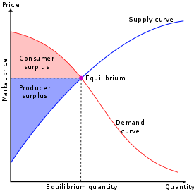
Graph illustrating consumer (red) and producer (blue) surpluses on a supply and demand chart

In mainstream economics, economic surplus, also known as total welfare or total social welfare or Marshallian surplus (after Alfred Marshall), is either of two related quantities:

• Consumer surplus, or consumers' surplus, is the monetary gain obtained by consumers because they are able to purchase a product for a price that is less than the highest price that they would be willing to pay.
• Producer surplus, or producers' surplus, is the amount that producers benefit by selling at a market price that is higher than the least that they would be willing to sell for; this is roughly equal to profit (since producers are not normally willing to sell at a loss and are normally indifferent to selling at a break-even price).

Overview

In the mid-19th century, engineer Jules Dupuit first propounded the concept of economic surplus, but it was the economist Alfred Marshall who gave the concept its fame in the field of economics.

On a standard supply and demand diagram, consumer surplus is the area (triangular if the supply and demand curves are linear) above the equilibrium price of the good and below the demand curve. This reflects the fact that consumers would have been willing to buy a single unit of the good at a price higher than the equilibrium price, a second unit at a price below that but still above the equilibrium price, etc., yet they in fact pay just the equilibrium price for each unit they buy.

Likewise, in the supply-demand diagram, producer surplus is the area below the equilibrium price but above the supply curve. This reflects the fact that producers would have been willing to supply the first unit at a price lower than the equilibrium price, the second unit at a price above that but still below the equilibrium price, etc., yet they in fact receive the equilibrium price for all the units they sell.

History

Early writers of economic issues used surplus as a means to draw conclusions about the relationship between production and necessities. In the agricultural sector surplus was an important concept because this sector has the responsibility to feed everyone plus itself. Food is notable because people only need a specific amount of food and can only consume a limited amount. This means that excess food production must overflow to other people, and will not be rationally hoarded. The non-agricultural sector is therefore limited by the agricultural sector equaling the output of food subtracting the amount consumed by the agricultural sector.

William Petty

William Petty  used a broad definition of necessities, leading him to focus on employment issues surrounding surplus. Petty explains a hypothetical example in which there is a territory of 1000 men and 100 of those men are capable of producing enough food for all 1000 men. The question becomes, what will the rest of the men do if only 100 are needed to provide necessities? He thereby suggests a variety of employments with some remaining unemployed.

David Hume

David Hume approached the agricultural surplus concept from another direction. Hume recognized that agriculture may feed more than those who cultivate it, but questioned why farmers would work to produce more than they need. Forceful production, which may occur under a feudal system, would be unlikely to generate a notable surplus in his opinion. Yet, if they could purchase luxuries and other goods beyond their necessities, they would become incentivized to produce and sell a surplus. Hume did not see this concept as abstract theory, he stated it as a fact when discussing how England developed after the introduction of foreign luxuries in his History of England.

Adam Smith

Adam Smith's thoughts on surplus drew on Hume. Smith noted that the desire for luxuries is infinite compared to the finite capacity of hunger. Smith saw the development in Europe as originating from landlords placing more importance on luxury spending rather than political power.

Consumer surplus

Consumer surplus is the difference between the maximum price a consumer is willing to pay and the actual price they do pay. If a consumer is willing to pay more for a unit of a good than the current asking price, they are getting more benefit from the purchased product than they would if the price was their maximum willingness to pay. They are receiving the same benefit, the obtainment of the good, at a lesser cost. An example of a good with generally high consumer surplus is drinking water. People would pay very high prices for drinking water, as they need it to survive. The difference in the price that they would pay, if they had to, and the amount that they pay now is their consumer surplus. The utility of the first few liters of drinking water is very high (as it prevents death), so the first few liters would likely have more consumer surplus than subsequent quantities.

The maximum amount a consumer would be willing to pay for a given quantity of a good is the sum of the maximum price they would pay for the first unit, the (lower) maximum price they would be willing to pay for the second unit, etc. Typically these prices are decreasing; they are given by the individual demand curve, which must be generated by a rational consumer who maximizes utility subject to a budget constraint. Because the demand curve is downward sloping, there is diminishing marginal utility. Diminishing marginal utility means a person receives less additional utility from an additional unit. However, the price of a product is constant for every unit at the equilibrium price. The extra money someone would be willing to pay for the number units of a product less than the equilibrium quantity and at a higher price than the equilibrium price for each of these quantities is the benefit they receive from purchasing these quantities. For a given price the consumer buys the amount for which the consumer surplus is highest. The consumer's surplus is highest at the largest number of units for which, even for the last unit, the maximum willingness to pay is not below the market price.

Consumer surplus can be used as a measurement of social welfare, shown by Robert Willig. For a single price change, consumer surplus can provide an approximation of changes in welfare. With multiple price and/or income changes, however, consumer surplus cannot be used to approximate economic welfare because it is not single-valued anymore. More modern methods are developed later to estimate the welfare effect of price changes using consumer surplus.

The aggregate consumers' surplus is the sum of the consumer's surplus for all individual consumers. This aggregation can be represented graphically, as shown in the above graph of the market demand and supply curves. The aggregate consumers' surplus can also be said to be the maxim of satisfaction a consumer derives from particular goods and services.

Calculation from supply and demand

The consumer surplus (individual or aggregated) is the area under the (individual or aggregated) demand curve and above a horizontal line at the actual price (in the aggregated case, the equilibrium price). If the demand curve is a straight line, the consumer surplus is the area of a triangle:

${\displaystyle CS=\frac{1}{2}{Q}_{\mathrm{m}\mathrm{k}\mathrm{t}}\left(P_{max}-P_{\mathrm{m}\mathrm{k}\mathrm{t}}\right),}$

where P_mkt is the equilibrium price (where supply equals demand), Q_mkt is the total quantity purchased at the equilibrium price, and P_max is the price at which the quantity purchased would fall to 0 (that is, where the demand curve intercepts the price axis). For more general demand and supply functions, these areas are not triangles but can still be found using integral calculus. Consumer surplus is thus the definite integral of the demand function with respect to price, from the market price to the maximum reservation price (i.e., the price-intercept of the demand function):

${\displaystyle CS={\int }_{P_{\mathrm{m}\mathrm{k}\mathrm{t}}}^{P_{max}}D(P)dP,}$

where ${\displaystyle D(P_{max})=0.}$ This shows that if we see a rise in the equilibrium price and a fall in the equilibrium quantity, then consumer surplus falls.

Calculation of a change in consumer surplus

The change in consumer surplus is used to measure the changes in prices and income. The demand function used to represent an individual's demand for a certain product is essential in determining the effects of a price change. An individual's demand function is a function of the individual's income, the demographic characteristics of the individual, and the vector of commodity prices. When the price of a product changes, the change in consumer surplus is measured as the negative value of the integral from the original actual price (P₀) and the new actual price (P₁) of the demand for product by the individual. If the change in consumer surplus is positive, the price change is said to have increased the individuals welfare. If the price change in consumer surplus is negative, the price change is said to have decreased the individual's welfare.

Distribution of benefits when price falls

When supply of a good expands, the price falls (assuming the demand curve is downward sloping) and consumer surplus increases. This benefits two groups of people: consumers who were already willing to buy at the initial price benefit from a price reduction, and they may buy more and receive even more consumer surplus; and additional consumers who were unwilling to buy at the initial price will buy at the new price and also receive some consumer surplus.

Consider an example of linear supply and demand curves. For an initial supply curve S₀, consumer surplus is the triangle above the line formed by price P₀ to the demand line (bounded on the left by the price axis and on the top by the demand line). If supply expands from S₀ to S₁, the consumers' surplus expands to the triangle above P₁ and below the demand line (still bounded by the price axis). The change in consumer's surplus is difference in area between the two triangles, and that is the consumer welfare associated with expansion of supply.

Some people were willing to pay the higher price P₀. When the price is reduced, their benefit is the area in the rectangle formed on the top by P₀, on the bottom by P₁, on the left by the price axis and on the right by line extending vertically upwards from Q₀.

The second set of beneficiaries are consumers who buy more, and new consumers, those who will pay the new lower price (P₁) but not the higher price (P₀). Their additional consumption makes up the difference between Q₁ and Q₀. Their consumer surplus is the triangle bounded on the left by the line extending vertically upwards from Q₀, on the right and top by the demand line, and on the bottom by the line extending horizontally to the right from P₁.

Rule of one-half

The rule of one-half estimates the change in consumer surplus for small changes in supply with a constant demand curve. Note that in the special case where the consumer demand curve is linear, consumer surplus is the area of the triangle bounded by the vertical line Q = 0, the horizontal line ${\displaystyle P=P_{\mathrm{m}\mathrm{k}\mathrm{t}}}$ and the linear demand curve. Hence, the change in consumer surplus is the area of the trapezoid with i) height equal to the change in price and ii) mid-segment length equal to the average of the ex-post and ex-ante equilibrium quantities. Following the figure above,

${\displaystyle \mathrm{\Delta }CS=\frac{1}{2}(Q_1+Q_0)(P_0-P_1),}$

where:

• CS = consumers' surplus;
• Q₀ and Q₁ are, respectively, the quantity demanded before and after a change in supply;
• P₀ and P₁ are, respectively, the prices before and after a change in supply.

Producer surplus

Producer surplus is the additional benefit that the owners of production factors and product providers bring to producers due to the differences between production, the supply price of the product, and the current market price. The difference between the amount actually obtained in a market transaction and the minimum amount it is willing to accept with the production factors or the products provided.

Calculation of producer surplus

Producer surplus is usually expressed by the area below the market price line and above the supply curve. In Figure 1, the shaded areas below the price line and above the supply curve between production zero and maximum output Q₁ indicate producer surplus. Among them, OP₁EQ₁ below the price line. This indicates that the total revenue is the minimum total payment actually accepted by the manufacturer. The area OP_MEQ₁ below the S curve is the minimum total revenue that the manufacturer is willing to accept. In Figure 1, the area enclosed by the market price line, the manufacturer's supply line, and the coordinate axis is the producer surplus. Because the rectangle OP₁EQ₁ is the total revenue actually obtained by the manufacturer, that is, A + B, and the trapezoid OP_MEQ. The minimum total profit that the manufacturer is willing to accept, that is, B, so A is the producer surplus.

Producer surplus

Obviously, the manufacturer produces and sells a certain quantity of Q₁ goods at the market price P₁. The manufacturer has reduced the quantity of goods for Q₁, which means that the manufacturer has increased the production factors or production costs equivalent to the amount of AVC·Q₁. However, at the same time, the manufacturer actually obtains a total income equivalent to the total market price P₁·Q₁. Since AVC is always smaller than P₁, from the production and sales of goods in Q₁, manufacturers not only get sales revenue equivalent to variable costs, but also get additional revenue. This part of the excess income reflects the increase in the benefits obtained by the manufacturers through market exchange. Therefore, in economics, producer surplus is usually used to measure producer welfare and is an important part of social welfare.

Producer surplus is usually used to measure the economic welfare obtained by the manufacturer in the market supply. When the supply price is constant, the producer welfare depends on the market price. If the manufacturer can sell the product at the highest price, the welfare is the greatest. As part of social welfare, the size of the producer surplus depends on many factors. Generally speaking, when other factors remain constant, an increase in market price will increase producer surplus, and a decrease in supply price or marginal cost will also increase producer surplus. If there is a surplus of goods, that is, people can only sell part of the goods at market prices, and producer surplus will decrease.

Obviously, the sum of the producer surplus of all manufacturers in the market constitutes the producer surplus of the entire market. Graphically, it should be expressed as the area enclosed by the market supply curve, the market price line and the coordinate axis.