Climate classification

From Wikipedia, the free encyclopedia
https://en.wikipedia.org/wiki/Climate_classification

Worldwide Köppen climate classifications

Climate classifications are systems that categorize the world's climates. A climate classification may correlate closely with a biome classification, as climate is a major influence on life in a region. One of the most used is the Köppen climate classification scheme first developed in 1899.

There are several ways to classify climates into similar regimes. Originally, climes were defined in Ancient Greece to describe the weather depending upon a location's latitude. Modern climate classification methods can be broadly divided into genetic methods, which focus on the causes of climate, and empiric methods, which focus on the effects of climate. Examples of genetic classification include methods based on the relative frequency of different air mass types or locations within synoptic weather disturbances. Examples of empiric classifications include climate zones defined by plant hardiness, evapotranspiration, or more generally the Köppen climate classification which was originally designed to identify the climates associated with certain biomes. A common shortcoming of these classification schemes is that they produce distinct boundaries between the zones they define, rather than the gradual transition of climate properties more common in nature.

Types of climate

• Alpine climate
• Desert climate or arid climate
• Humid continental climate
• Humid subtropical climate
• Ice cap climate
• Oceanic climate
• Subarctic climate
• Semi-arid climate
• Mediterranean climate
• Tropical monsoon climate
• Tropical rainforest climate
• Tropical savanna climate
• Tundra climate
• Polar climate

Systems

Leslie Holdridge's Life Zone Classification system is essentially a climate classification scheme.

Climate classification systems include:

• Aridity index – part of many systems
• Alisov climate classification (ru)
• Berg climate classification
• Köppen climate classification – most widely used in the 1954 Köppen–Geiger variant
• Holdridge life zone classification – relatively simple
• Lauer climate classification
• Strahler climate classification
• Thornthwaite climate classification
• Trewartha climate classification – 1967 modification of Köppen to fit real-world conditions
• Troll climate classification
• Vahl climate classification

Bergeron and Spatial Synoptic

The simplest classification is that involving air masses. The Bergeron classification is the most widely accepted form of air mass classification. Air mass classification involves three letters. The first letter describes its moisture properties, with c used for continental air masses (dry) and m for maritime air masses (moist). The second letter describes the thermal characteristic of its source region: T for tropical, P for polar, A for Arctic or Antarctic, M for monsoon, E for equatorial, and S for superior air (dry air formed by significant downward motion in the atmosphere). The third letter is used to designate the stability of the atmosphere. If the air mass is colder than the ground below it, it is labeled k. If the air mass is warmer than the ground below it, it is labeled w. While air mass identification was originally used in weather forecasting during the 1950s, climatologists began to establish synoptic climatologies based on this idea in 1973.

Based upon the Bergeron classification scheme is the Spatial Synoptic Classification system (SSC). There are six categories within the SSC scheme: Dry Polar (similar to continental polar), Dry Moderate (similar to maritime superior), Dry Tropical (similar to continental tropical), Moist Polar (similar to maritime polar), Moist Moderate (a hybrid between maritime polar and maritime tropical), and Moist Tropical (similar to maritime tropical, maritime monsoon, or maritime equatorial).

Köppen

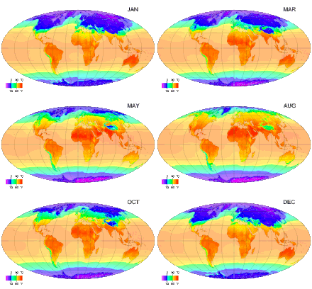
Monthly average surface temperatures from 1961 to 1990. This is an example of how climate varies with location and season

 

Monthly global images from NASA Earth Observatory (interactive SVG)

 

Main article: Köppen climate classification

The Köppen classification depends on average monthly values of temperature and precipitation. The most commonly used form of the Köppen classification has five primary types labeled A through E. These primary types are A) tropical, B) dry, C) mild mid-latitude, D) cold mid-latitude, and E) polar.

Tropical climates are defined as locations where the coolest monthly mean temperature is above 18 C (64.4 F). This tropical zone is further broken down into rainforest, monsoon, and savanna based on seasonal rainfall. These climates are most often located between the Equator and 25 north and south latitude.

A monsoon is a seasonal prevailing wind which lasts for several months, ushering in a region's rainy season. Regions within North America, South America, Sub-Saharan Africa, Australia and East Asia are monsoon regimes.

The world's cloudy and sunny spots. NASA Earth Observatory map using data collected between July 2002 and April 2015.

A tropical savanna is a grassland biome located in semi-arid to semi-humid climate regions of subtropical and tropical latitudes, with average temperatures remaining at or above 18 °C (64 °F) all year round, and rainfall between 750 millimetres (30 in) and 1,270 millimetres (50 in) a year. They are widespread on Africa, and are found in India, the northern parts of South America, Malaysia, and Australia.

Cloud cover by month for 2014. NASA Earth Observatory

The humid subtropical climate zone where winter rainfall (and sometimes light snowfall) is associated with storms that the westerlies steer from west to east at the time of low sun (winter). In summer, high pressure dominates as the westerlies move north. Most summer rainfall occurs during thunderstorms and from occasional tropical cyclones. Humid subtropical climates lie on the east side of continents, roughly between latitudes 20° and 40° degrees away from the equator.

Humid continental climate, worldwide

A humid continental climate is marked by variable weather patterns and a large seasonal temperature variance, cold and often very snowy winters, and warm summers. Places with more than three months of average daily temperatures above 10 °C (50 °F) and a coldest month temperature below −3 °C (27 °F) and which do not meet the criteria for an arid or semi-arid climate, are classified as continental. Most climates in this zone are found from 35 latitude to 55 latitude, mostly in the northern hemisphere.

An oceanic climate is typically found along west coasts in higher middle latitudes of all the world's continents, and in southeastern Australia, and is accompanied by plentiful precipitation year-round, cool summers, and small annual ranges of temperatures. Most climates of this type are found from 45 latitude to 55 latitude.

The Mediterranean climate regime resembles the climate of the lands in the Mediterranean Basin, parts of western North America, parts of Western and South Australia, in southwestern South Africa and in parts of central Chile. The climate is characterized by hot, dry summers and cool, wet winters.

A steppe is a dry grassland with an annual temperature range in the summer of up to 40 °C (104 °F) and during the winter down to −40 °C (−40 °F).

A subarctic climate has little precipitation, and monthly temperatures which are above 10 °C (50 °F) for one to three months of the year, with permafrost in large parts of the area due to the cold winters. Winters within subarctic climates usually include up to six months of temperatures averaging below 0 °C (32 °F).

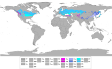
Map of arctic tundra

Tundra occurs in the far Northern Hemisphere, north of the taiga belt, including vast areas of northern Russia and Canada.

A polar ice cap, or polar ice sheet, is a high-latitude region of a planet or moon that is covered in ice. Ice caps form because high-latitude regions receive less energy as solar radiation from the sun than equatorial regions, resulting in lower surface temperatures.

A desert is a landscape form or region that receives very little precipitation. Deserts usually have a large diurnal and seasonal temperature range, with high or low, depending on location daytime temperatures (in summer up to 45 °C or 113 °F), and low nighttime temperatures (in winter down to 0 °C or 32 °F) due to extremely low humidity. Many deserts are formed by rain shadows, as mountains block the path of moisture and precipitation to the desert.

Trewartha

The Trewartha climate classification (TCC) or the Köppen–Trewartha climate classification (KTC) is a climate classification system first published by American geographer Glenn Thomas Trewartha in 1966. It is a modified version of the Köppen–Geiger system, created to answer some of its deficiencies. The Trewartha system attempts to redefine the middle latitudes to be closer to vegetation zoning and genetic climate systems. It was considered a more true or "real world" reflection of the global climate.

The Trewartha climate classification changes were seen as most effective on the large landmasses in Asia and North America, where many areas fall into a single group (C) in the Köppen–Geiger system. For example, under the standard Köppen system, Washington and Oregon are classed into the same climate zone (Csb) as parts of Southern California, even though the two regions have strikingly different weather and vegetation. Another example was classifying cities like London or Chicago in the same climate group (C) as Brisbane or New Orleans, despite great differences in seasonal temperatures and native plant life.

Scheme

Trewartha's modifications to the 1899 Köppen climate system sought to reclass the middle latitudes into three groups: C (subtropical)—8 or more months have a mean temperature of 10 °C (50 °F) or higher; D temperate—4 to 7 months have a mean temperature of 10 °C or higher; and E boreal climate—1 to 3 months have a mean temperature of 10 °C or higher. Otherwise, the tropical climates and polar climates remained the same as the original Köppen climate classification.

Thornthwaite

Main article: Thornthwaite climate classification

See also: Microthermal, Mesothermal, and Megathermal

 

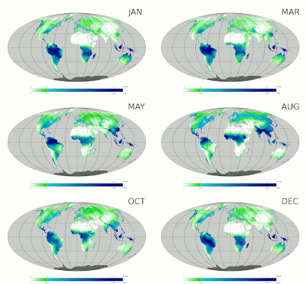
Precipitation by month

Devised by the American climatologist and geographer C. W. Thornthwaite, this climate classification method monitors the soil water budget using evapotranspiration. It monitors the portion of total precipitation used to nourish vegetation over a certain area. It uses indices such as a humidity index and an aridity index to determine an area's moisture regime based upon its average temperature, average rainfall, and average vegetation type. The lower the value of the index in any given area, the drier the area is.

The moisture classification includes climatic classes with descriptors such as hyperhumid, humid, subhumid, subarid, semi-arid (values of −20 to −40), and arid (values below −40). Humid regions experience more precipitation than evaporation each year, while arid regions experience greater evaporation than precipitation on an annual basis. A total of 33 percent of the Earth's landmass is considered either arid or semi-arid, including southwest North America, southwest South America, most of northern and a small part of southern Africa, southwest and portions of eastern Asia, as well as much of Australia. Studies suggest that precipitation effectiveness (PE) within the Thornthwaite moisture index is overestimated in the summer and underestimated in the winter. This index can be effectively used to determine the number of herbivore and mammal species numbers within a given area. The index is also used in studies of climate change.

Thermal classifications within the Thornthwaite scheme include microthermal, mesothermal, and megathermal regimes. A microthermal climate is one of low annual mean temperatures, generally between 0 °C (32 °F) and 14 °C (57 °F) which experiences short summers and has a potential evaporation between 14 centimetres (5.5 in) and 43 centimetres (17 in). A mesothermal climate lacks persistent heat or persistent cold, with potential evaporation between 57 centimetres (22 in) and 114 centimetres (45 in). A megathermal climate is one with persistent high temperatures and abundant rainfall, with potential annual evaporation in excess of 114 centimetres (45 in).

Adiabatic theorem

From Wikipedia, the free encyclopedia

https://en.wikipedia.org/wiki/Adiabatic_theorem

The adiabatic theorem is a concept in quantum mechanics. Its original form, due to Max Born and Vladimir Fock (1928), was stated as follows:

A physical system remains in its instantaneous eigenstate if a given perturbation is acting on it slowly enough and if there is a gap between the eigenvalue and the rest of the Hamiltonian's spectrum.

In simpler terms, a quantum mechanical system subjected to gradually changing external conditions adapts its functional form, but when subjected to rapidly varying conditions there is insufficient time for the functional form to adapt, so the spatial probability density remains unchanged.

Diabatic vs. adiabatic processes

Comparison

Diabatic	Adiabatic
Rapidly changing conditions prevent the system from adapting its configuration during the process, hence the spatial probability density remains unchanged. Typically there is no eigenstate of the final Hamiltonian with the same functional form as the initial state. The system ends in a linear combination of states that sum to reproduce the initial probability density.	Gradually changing conditions allow the system to adapt its configuration, hence the probability density is modified by the process. If the system starts in an eigenstate of the initial Hamiltonian, it will end in the corresponding eigenstate of the final Hamiltonian.

At some initial time ${\displaystyle t_0}$ a quantum-mechanical system has an energy given by the Hamiltonian ${\displaystyle \hat{H}(t_0)}$; the system is in an eigenstate of ${\displaystyle \hat{H}(t_0)}$ labelled ${\displaystyle \psi (x,t_0)}$. Changing conditions modify the Hamiltonian in a continuous manner, resulting in a final Hamiltonian ${\displaystyle \hat{H}(t_1)}$ at some later time ${\displaystyle t_1}$. The system will evolve according to the time-dependent Schrödinger equation, to reach a final state ${\displaystyle \psi (x,t_1)}$. The adiabatic theorem states that the modification to the system depends critically on the time ${\displaystyle \tau =t_1-t_0}$ during which the modification takes place.

For a truly adiabatic process we require ${\displaystyle \tau \to \mathrm{\infty }}$; in this case the final state ${\displaystyle \psi (x,t_1)}$ will be an eigenstate of the final Hamiltonian ${\displaystyle \hat{H}(t_1)}$, with a modified configuration:

${\displaystyle |\psi (x,t_1){|}^2\ne |\psi (x,t_0){|}^2.}$

The degree to which a given change approximates an adiabatic process depends on both the energy separation between ${\displaystyle \psi (x,t_0)}$ and adjacent states, and the ratio of the interval ${\displaystyle \tau }$ to the characteristic time-scale of the evolution of ${\displaystyle \psi (x,t_0)}$ for a time-independent Hamiltonian, ${\displaystyle {\tau }_{int}=2\pi \hslash /E_0}$, where ${\displaystyle E_0}$ is the energy of ${\displaystyle \psi (x,t_0)}$.

Conversely, in the limit ${\displaystyle \tau \to 0}$ we have infinitely rapid, or diabatic passage; the configuration of the state remains unchanged:

${\displaystyle |\psi (x,t_1){|}^2=|\psi (x,t_0){|}^2.}$

The so-called "gap condition" included in Born and Fock's original definition given above refers to a requirement that the spectrum of ${\displaystyle \hat{H}}$ is discrete and nondegenerate, such that there is no ambiguity in the ordering of the states (one can easily establish which eigenstate of ${\displaystyle \hat{H}(t_1)}$ corresponds to ${\displaystyle \psi (t_0)}$). In 1999 J. E. Avron and A. Elgart reformulated the adiabatic theorem to adapt it to situations without a gap.

Comparison with the adiabatic concept in thermodynamics

The term "adiabatic" is traditionally used in thermodynamics to describe processes without the exchange of heat between system and environment (see adiabatic process), more precisely these processes are usually faster than the timescale of heat exchange. (For example, a pressure wave is adiabatic with respect to a heat wave, which is not adiabatic.) Adiabatic in the context of thermodynamics is often used as a synonym for fast process.

The classical and quantum mechanics definition is closer instead to the thermodynamical concept of a quasistatic process, which are processes that are almost always at equilibrium (i.e. that are slower than the internal energy exchange interactions time scales, namely a "normal" atmospheric heat wave is quasi-static and a pressure wave is not). Adiabatic in the context of Mechanics is often used as a synonym for slow process.

In the quantum world adiabatic means for example that the time scale of electrons and photon interactions is much faster or almost instantaneous with respect to the average time scale of electrons and photon propagation. Therefore, we can model the interactions as a piece of continuous propagation of electrons and photons (i.e. states at equilibrium) plus a quantum jump between states (i.e. instantaneous).

The adiabatic theorem in this heuristic context tells essentially that quantum jumps are preferably avoided and the system tries to conserve the state and the quantum numbers.

The quantum mechanical concept of adiabatic is related to adiabatic invariant, it is often used in the old quantum theory and has no direct relation with heat exchange.

Example systems

Simple pendulum

As an example, consider a pendulum oscillating in a vertical plane. If the support is moved, the mode of oscillation of the pendulum will change. If the support is moved sufficiently slowly, the motion of the pendulum relative to the support will remain unchanged. A gradual change in external conditions allows the system to adapt, such that it retains its initial character. The detailed classical example is available in the Adiabatic invariant page and here.

Quantum harmonic oscillator

Figure 1. Change in the probability density, ${\displaystyle |\psi (t){|}^2}$, of a ground state quantum harmonic oscillator, due to an adiabatic increase in spring constant.

The classical nature of a pendulum precludes a full description of the effects of the adiabatic theorem. As a further example consider a quantum harmonic oscillator as the spring constant ${\displaystyle k}$ is increased. Classically this is equivalent to increasing the stiffness of a spring; quantum-mechanically the effect is a narrowing of the potential energy curve in the system Hamiltonian.

If ${\displaystyle k}$ is increased adiabatically $\left(\frac{dk}{dt}\to 0\right)$ then the system at time ${\displaystyle t}$ will be in an instantaneous eigenstate ${\displaystyle \psi (t)}$ of the current Hamiltonian ${\displaystyle \hat{H}(t)}$, corresponding to the initial eigenstate of ${\displaystyle \hat{H}(0)}$. For the special case of a system like the quantum harmonic oscillator described by a single quantum number, this means the quantum number will remain unchanged. Figure 1 shows how a harmonic oscillator, initially in its ground state, ${\displaystyle n=0}$, remains in the ground state as the potential energy curve is compressed; the functional form of the state adapting to the slowly varying conditions.

For a rapidly increased spring constant, the system undergoes a diabatic process $\left(\frac{dk}{dt}\to \mathrm{\infty }\right)$ in which the system has no time to adapt its functional form to the changing conditions. While the final state must look identical to the initial state ${\displaystyle \left(|\psi (t){|}^2=|\psi (0){|}^2\right)}$ for a process occurring over a vanishing time period, there is no eigenstate of the new Hamiltonian, ${\displaystyle \hat{H}(t)}$, that resembles the initial state. The final state is composed of a linear superposition of many different eigenstates of ${\displaystyle \hat{H}(t)}$ which sum to reproduce the form of the initial state.

Avoided curve crossing

Main article: Avoided crossing

 

Figure 2. An avoided energy-level crossing in a two-level system subjected to an external magnetic field. Note the energies of the diabatic states, ${\displaystyle |1⟩}$ and ${\displaystyle |2⟩}$ and the eigenvalues of the Hamiltonian, giving the energies of the eigenstates ${\displaystyle |{\varphi }_1⟩}$ and ${\displaystyle |{\varphi }_2⟩}$ (the adiabatic states). (Actually, ${\displaystyle |{\varphi }_1⟩}$ and ${\displaystyle |{\varphi }_2⟩}$ should be switched in this picture.)

For a more widely applicable example, consider a 2-level atom subjected to an external magnetic field. The states, labelled ${\displaystyle |1⟩}$ and ${\displaystyle |2⟩}$ using bra–ket notation, can be thought of as atomic angular-momentum states, each with a particular geometry. For reasons that will become clear these states will henceforth be referred to as the diabatic states. The system wavefunction can be represented as a linear combination of the diabatic states:

${\displaystyle |\mathrm{\Psi }⟩=c_1(t)|1⟩+c_2(t)|2⟩.}$

With the field absent, the energetic separation of the diabatic states is equal to ${\displaystyle \hslash {\omega }_0}$; the energy of state ${\displaystyle |1⟩}$ increases with increasing magnetic field (a low-field-seeking state), while the energy of state ${\displaystyle |2⟩}$ decreases with increasing magnetic field (a high-field-seeking state). Assuming the magnetic-field dependence is linear, the Hamiltonian matrix for the system with the field applied can be written

${\displaystyle \mathbf{H}=\left(\begin{array}{cc}\mu B(t)-\hslash {\omega }_0/2& a\\ a^{\ast }& \hslash {\omega }_0/2-\mu B(t)\end{array}\right)}$

where ${\displaystyle \mu }$ is the magnetic moment of the atom, assumed to be the same for the two diabatic states, and ${\displaystyle a}$ is some time-independent coupling between the two states. The diagonal elements are the energies of the diabatic states (${\displaystyle E_1(t)}$ and ${\displaystyle E_2(t)}$), however, as ${\displaystyle \mathbf{H}}$ is not a diagonal matrix, it is clear that these states are not eigenstates of the new Hamiltonian that includes the magnetic field contribution.

The eigenvectors of the matrix ${\displaystyle \mathbf{H}}$ are the eigenstates of the system, which we will label ${\displaystyle |{\varphi }_1(t)⟩}$ and ${\displaystyle |{\varphi }_2(t)⟩}$, with corresponding eigenvalues

$${\displaystyle \begin{array}{rl}{\epsilon }_1(t)& =-\frac{1}{2}\sqrt{4a^2+(\hslash {\omega }_0-2\mu B(t){)}^2}\\ {\epsilon }_2(t)& =+\frac{1}{2}\sqrt{4a^2+(\hslash {\omega }_0-2\mu B(t){)}^2}.\end{array}}$$

It is important to realise that the eigenvalues ${\displaystyle {\epsilon }_1(t)}$ and ${\displaystyle {\epsilon }_2(t)}$ are the only allowed outputs for any individual measurement of the system energy, whereas the diabatic energies ${\displaystyle E_1(t)}$ and ${\displaystyle E_2(t)}$ correspond to the expectation values for the energy of the system in the diabatic states ${\displaystyle |1⟩}$ and ${\displaystyle |2⟩}$.

Figure 2 shows the dependence of the diabatic and adiabatic energies on the value of the magnetic field; note that for non-zero coupling the eigenvalues of the Hamiltonian cannot be degenerate, and thus we have an avoided crossing. If an atom is initially in state ${\displaystyle |{\varphi }_2(t_0)⟩}$ in zero magnetic field (on the red curve, at the extreme left), an adiabatic increase in magnetic field $\left(\frac{dB}{dt}\to 0\right)$ will ensure the system remains in an eigenstate of the Hamiltonian ${\displaystyle |{\varphi }_2(t)⟩}$ throughout the process (follows the red curve). A diabatic increase in magnetic field $\left(\frac{dB}{dt}\to \mathrm{\infty }\right)$ will ensure the system follows the diabatic path (the dotted blue line), such that the system undergoes a transition to state ${\displaystyle |{\varphi }_1(t_1)⟩}$. For finite magnetic field slew rates $\left(0<\frac{dB}{dt}<\mathrm{\infty }\right)$ there will be a finite probability of finding the system in either of the two eigenstates. See below for approaches to calculating these probabilities.

These results are extremely important in atomic and molecular physics for control of the energy-state distribution in a population of atoms or molecules.

Mathematical statement

Under a slowly changing Hamiltonian ${\displaystyle H(t)}$ with instantaneous eigenstates ${\displaystyle |n(t)⟩}$ and corresponding energies ${\displaystyle E_n(t)}$, a quantum system evolves from the initial state

$${\displaystyle |\psi (0)⟩=\sum _n{c}_n(0)|n(0)⟩}$$

to the final state

$${\displaystyle |\psi (t)⟩=\sum _n{c}_n(t)|n(t)⟩,}$$

where the coefficients undergo the change of phase

$${\displaystyle c_n(t)=c_n(0)e^{i{\theta }_n(t)}{e}^{i{\gamma }_n(t)}}$$

with the dynamical phase

$${\displaystyle {\theta }_m(t)=\frac{-1}{\hslash }{\int }_0^t{E}_m(t^{\prime })d{t}^{\prime }}$$

and geometric phase

$${\displaystyle {\gamma }_m(t)=i{\int }_0^t⟨m(t^{\prime })|\dot{m}(t^{\prime })⟩d{t}^{\prime }.}$$

In particular, ${\displaystyle |c_n(t){|}^2=|c_n(0){|}^2}$, so if the system begins in an eigenstate of ${\displaystyle H(0)}$, it remains in an eigenstate of ${\displaystyle H(t)}$ during the evolution with a change of phase only.

Example applications

Often a solid crystal is modeled as a set of independent valence electrons moving in a mean perfectly periodic potential generated by a rigid lattice of ions. With the Adiabatic theorem we can also include instead the motion of the valence electrons across the crystal and the thermal motion of the ions as in the Born–Oppenheimer approximation.

This does explain many phenomena in the scope of:

• thermodynamics: Temperature dependence of specific heat, thermal expansion, melting
• transport phenomena: the temperature dependence of electric resistivity of conductors, the temperature dependence of electric conductivity in insulators, Some properties of low temperature superconductivity
• optics: optic absorption in the infrared for ionic crystals, Brillouin scattering, Raman scattering

Deriving conditions for diabatic vs adiabatic passage

We will now pursue a more rigorous analysis. Making use of bra–ket notation, the state vector of the system at time ${\displaystyle t}$ can be written

${\displaystyle |\psi (t)⟩=\sum _n{c}_n^A(t)e^{-i{E}_{n}t/\hslash }|{\varphi }_n⟩,}$

where the spatial wavefunction alluded to earlier is the projection of the state vector onto the eigenstates of the position operator

${\displaystyle \psi (x,t)=⟨x|\psi (t)⟩.}$

It is instructive to examine the limiting cases, in which ${\displaystyle \tau }$ is very large (adiabatic, or gradual change) and very small (diabatic, or sudden change).

Consider a system Hamiltonian undergoing continuous change from an initial value ${\displaystyle {\hat{H}}_0}$, at time ${\displaystyle t_0}$, to a final value ${\displaystyle {\hat{H}}_1}$, at time ${\displaystyle t_1}$, where ${\displaystyle \tau =t_1-t_0}$. The evolution of the system can be described in the Schrödinger picture by the time-evolution operator, defined by the integral equation

${\displaystyle \hat{U}(t,t_0)=1-\frac{i}{\hslash }{\int }_{t_0}^t\hat{H}(t^{\prime })\hat{U}(t^{\prime },t_0)d{t}^{\prime },}$

which is equivalent to the Schrödinger equation.

${\displaystyle i\hslash \frac{\mathrm{\partial }}{\mathrm{\partial }t}\hat{U}(t,t_0)=\hat{H}(t)\hat{U}(t,t_0),}$

along with the initial condition ${\displaystyle \hat{U}(t_0,t_0)=1}$. Given knowledge of the system wave function at ${\displaystyle t_0}$, the evolution of the system up to a later time ${\displaystyle t}$ can be obtained using

${\displaystyle |\psi (t)⟩=\hat{U}(t,t_0)|\psi (t_0)⟩.}$

The problem of determining the adiabaticity of a given process is equivalent to establishing the dependence of ${\displaystyle \hat{U}(t_1,t_0)}$ on ${\displaystyle \tau }$.

To determine the validity of the adiabatic approximation for a given process, one can calculate the probability of finding the system in a state other than that in which it started. Using bra–ket notation and using the definition ${\displaystyle |0⟩\equiv |\psi (t_0)⟩}$, we have:

${\displaystyle \zeta =⟨0|{\hat{U}}^{†}(t_1,t_0)\hat{U}(t_1,t_0)|0⟩-⟨0|{\hat{U}}^{†}(t_1,t_0)|0⟩⟨0|\hat{U}(t_1,t_0)|0⟩.}$

We can expand ${\displaystyle \hat{U}(t_1,t_0)}$

${\displaystyle \hat{U}(t_1,t_0)=1+\frac{1}{i\hslash }{\int }_{t_0}^{t_1}\hat{H}(t)dt+\frac{1}{(i\hslash {)}^2}{\int }_{t_0}^{t_1}d{t}^{\prime }{\int }_{t_0}^{t^{\prime }}d{t}^{″}\hat{H}(t^{\prime })\hat{H}(t^{″})+\cdots .}$

In the perturbative limit we can take just the first two terms and substitute them into our equation for ${\displaystyle \zeta }$, recognizing that

${\displaystyle \frac{1}{\tau }{\int }_{t_0}^{t_1}\hat{H}(t)dt\equiv \overline{H}}$

is the system Hamiltonian, averaged over the interval ${\displaystyle t_0\to t_1}$, we have:

${\displaystyle \zeta =⟨0|(1+\frac{i}{\hslash }\tau \overline{H})(1-\frac{i}{\hslash }\tau \overline{H})|0⟩-⟨0|(1+\frac{i}{\hslash }\tau \overline{H})|0⟩⟨0|(1-\frac{i}{\hslash }\tau \overline{H})|0⟩.}$

After expanding the products and making the appropriate cancellations, we are left with:

${\displaystyle \zeta =\frac{{\tau }^2}{{\hslash }^2}\left(⟨0|{\overline{H}}^2|0⟩-⟨0|\overline{H}|0⟩⟨0|\overline{H}|0⟩\right),}$

giving

${\displaystyle \zeta =\frac{{\tau }^2\mathrm{\Delta }{\overline{H}}^2}{{\hslash }^2},}$

where ${\displaystyle \mathrm{\Delta }\overline{H}}$ is the root mean square deviation of the system Hamiltonian averaged over the interval of interest.

The sudden approximation is valid when ${\displaystyle \zeta \ll 1}$ (the probability of finding the system in a state other than that in which is started approaches zero), thus the validity condition is given by

${\displaystyle \tau \ll \frac{\hslash }{\mathrm{\Delta }\overline{H}},}$

which is a statement of the time-energy form of the Heisenberg uncertainty principle.

Diabatic passage

In the limit ${\displaystyle \tau \to 0}$ we have infinitely rapid, or diabatic passage:

${\displaystyle \underset{\tau \to 0}{lim}\hat{U}(t_1,t_0)=1.}$

The functional form of the system remains unchanged:

${\displaystyle |⟨x|\psi (t_1)⟩{|}^2={\left|⟨x|\psi (t_0)⟩\right|}^2.}$

This is sometimes referred to as the sudden approximation. The validity of the approximation for a given process can be characterized by the probability that the state of the system remains unchanged:

${\displaystyle P_D=1-\zeta .}$

Adiabatic passage

In the limit ${\displaystyle \tau \to \mathrm{\infty }}$ we have infinitely slow, or adiabatic passage. The system evolves, adapting its form to the changing conditions,

${\displaystyle |⟨x|\psi (t_1)⟩{|}^2\ne |⟨x|\psi (t_0)⟩{|}^2.}$

If the system is initially in an eigenstate of ${\displaystyle \hat{H}(t_0)}$, after a period ${\displaystyle \tau }$ it will have passed into the corresponding eigenstate of ${\displaystyle \hat{H}(t_1)}$.

This is referred to as the adiabatic approximation. The validity of the approximation for a given process can be determined from the probability that the final state of the system is different from the initial state:

${\displaystyle P_A=\zeta .}$

Calculating adiabatic passage probabilities

The Landau–Zener formula

Main article: Landau–Zener formula

In 1932 an analytic solution to the problem of calculating adiabatic transition probabilities was published separately by Lev Landau and Clarence Zener, for the special case of a linearly changing perturbation in which the time-varying component does not couple the relevant states (hence the coupling in the diabatic Hamiltonian matrix is independent of time).

The key figure of merit in this approach is the Landau–Zener velocity:

$${\displaystyle v_{\text{LZ}}=\frac{\frac{\mathrm{\partial }}{\mathrm{\partial }t}|E_2-E_1|}{\frac{\mathrm{\partial }}{\mathrm{\partial }q}|E_2-E_1|}\approx \frac{dq}{dt},}$$

where ${\displaystyle q}$ is the perturbation variable (electric or magnetic field, molecular bond-length, or any other perturbation to the system), and ${\displaystyle E_1}$ and ${\displaystyle E_2}$ are the energies of the two diabatic (crossing) states. A large ${\displaystyle v_{\text{LZ}}}$ results in a large diabatic transition probability and vice versa.

Using the Landau–Zener formula the probability, ${\displaystyle P_{\mathrm{D}}}$, of a diabatic transition is given by

$${\displaystyle \begin{array}{rl}{P}_{\mathrm{D}}& =e^{-2\pi \mathrm{\Gamma }}\\ \mathrm{\Gamma }& =\frac{a^2/\hslash }{\left|\frac{\mathrm{\partial }}{\mathrm{\partial }t}(E_2-E_1)\right|}=\frac{a^2/\hslash }{\left|\frac{dq}{dt}\frac{\mathrm{\partial }}{\mathrm{\partial }q}(E_2-E_1)\right|}\\ & =\frac{a^2}{\hslash |\alpha |}\end{array}}$$

The numerical approach

Main article: Numerical solution of ordinary differential equations

For a transition involving a nonlinear change in perturbation variable or time-dependent coupling between the diabatic states, the equations of motion for the system dynamics cannot be solved analytically. The diabatic transition probability can still be obtained using one of the wide variety of numerical solution algorithms for ordinary differential equations.

The equations to be solved can be obtained from the time-dependent Schrödinger equation:

$${\displaystyle i\hslash {\dot{\underset{\_}{c}}}^A(t)={\mathbf{H}}_A(t){\underset{\_}{c}}^A(t),}$$

where ${\displaystyle {\underset{\_}{c}}^A(t)}$ is a vector containing the adiabatic state amplitudes, ${\displaystyle {\mathbf{H}}_A(t)}$ is the time-dependent adiabatic Hamiltonian, and the overdot represents a time derivative.

Comparison of the initial conditions used with the values of the state amplitudes following the transition can yield the diabatic transition probability. In particular, for a two-state system:

$${\displaystyle P_D=|c_2^A(t_1){|}^2}$$

for a system that began with ${\displaystyle |c_1^A(t_0){|}^2=1}$.