Computer simulation of the
Earth's field in a period of
normal polarity between reversals.
[1] The lines represent magnetic field lines, blue when the field points towards the center and yellow when away. The rotation axis of the Earth is centered and vertical. The dense clusters of lines are within the Earth's core.
[2]
Earth's magnetic field, also known as the
geomagnetic field, is the
magnetic field that extends from the
Earth's interior to where it meets the
solar wind, a stream of
charged particles emanating from the
Sun. Its magnitude at the Earth's surface ranges from 25 to 65
microteslas (0.25 to 0.65
gauss).
[3] Roughly speaking it is the field of a
magnetic dipole currently tilted at an angle of about 10 degrees with respect to
Earth's rotational axis, as if there were a
bar magnet placed at that angle at the center of the Earth. Unlike a bar magnet, however, Earth's magnetic field changes over time because it is generated by a
geodynamo (in Earth's case, the motion of molten iron alloys in its
outer core).
The North and South
magnetic poles wander widely, but sufficiently slowly for ordinary
compasses to remain useful for navigation. However, at irregular intervals averaging several hundred thousand years,
the Earth's field reverses and the North and
South Magnetic Poles relatively abruptly switch places. These reversals of the
geomagnetic poles leave a record in rocks that are of value to
paleomagnetists in calculating geomagnetic fields in the past. Such information in turn is helpful in studying the motions of continents and ocean floors in the process of
plate tectonics.
The
magnetosphere is the region above the
ionosphere and extends several tens of thousands of kilometers into
space, protecting the Earth from the charged particles of the solar wind and
cosmic rays that would otherwise strip away the upper atmosphere, including the
ozone layer that protects the Earth from
harmful ultraviolet radiation.
Importance
Earth's magnetic field serves to deflect most of the solar wind, whose charged particles would otherwise strip away the ozone layer that protects the Earth from harmful ultraviolet radiation.
[4] One stripping mechanism is for gas to be caught in bubbles of magnetic field, which are ripped off by solar winds.
[5] Calculations of the loss of carbon dioxide from the atmosphere of
Mars, resulting from scavenging of ions by the solar wind, indicate that the dissipation of the magnetic field of Mars caused a near-total loss of its atmosphere.
[6][7]
The study of past magnetic field of the Earth is known as
paleomagnetism.
[8] The polarity of the Earth's magnetic field is recorded in
igneous rocks, and
reversals of the field are thus detectable as "stripes" centered on
mid-ocean ridges where the
sea floor is spreading, while the stability of the
geomagnetic poles between reversals has allowed paleomagnetists to track the past motion of continents. Reversals also provide the basis for
magnetostratigraphy, a way of
dating rocks and sediments.
[9] The field also magnetizes the crust, and
magnetic anomalies can be used to search for deposits of metal
ores.
[10]
Humans have used
compasses for direction finding since the 11th century A.D. and for navigation since the 12th century.
[11] Although the
magnetic declination does shift with time, this wandering is slow enough that a simple
compass remains useful for navigation. Using
magnetoception various other organisms, ranging from soil bacteria to pigeons, can detect the magnetic field and use it for navigation.
Main characteristics
Description
At any location, the Earth's magnetic field can be represented by a three-dimensional vector (see figure). A typical procedure for measuring its direction is to use a compass to determine the direction of magnetic North. Its angle relative to true North is the
declination (
D) or
variation. Facing magnetic North, the angle the field makes with the horizontal is the
inclination (
I) or
magnetic dip. The
intensity (
F) of the field is proportional to the force it exerts on a magnet. Another common representation is in
X (North),
Y (East) and
Z (Down) coordinates.
[12]

Common coordinate systems used for representing the Earth's magnetic field.
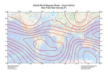
Intensity
The intensity of the field is often measured in
gauss (G), but is generally reported in
nanoteslas (nT), with 1 G = 100,000 nT. A nanotesla is also referred to as a gamma (γ).
[13] The
tesla is the
SI unit of the
Magnetic field,
B. The field ranges between approximately 25,000 and 65,000 nT (0.25–0.65 G). By comparison, a strong
refrigerator magnet has a field of about 100 gauss (0.010 T).
[14]
A map of intensity contours is called an
isodynamic chart. As the
2010 World Magnetic Model shows, the intensity tends to decrease from the poles to the equator. A minimum intensity occurs over South America while there are maxima over northern Canada, Siberia, and the coast of Antarctica south of Australia.
[15]
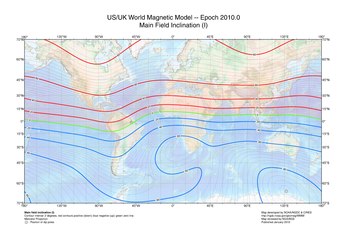
Inclination
The inclination is given by an angle that can assume values between -90° (up) to 90° (down). In the northern hemisphere, the field points downwards. It is straight down at the
North Magnetic Pole and rotates upwards as the latitude decreases until it is horizontal (0°) at the magnetic equator. It continues to rotate upwards until it is straight up at the
South Magnetic Pole. Inclination can be measured with a
dip circle.
An
isoclinic chart (map of inclination contours) for the Earth's magnetic field is shown
below.
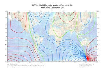
Declination
Declination is positive for an eastward deviation of the field relative to true north. It can be estimated by comparing the magnetic north/south heading on a compass with the direction of a
celestial pole. Maps typically include information on the declination as an angle or a small diagram showing the relationship between magnetic north and true north. Information on declination for a region can be represented by a chart with isogonic lines (contour lines with each line representing a fixed declination).
Geographical variation
Components of the Earth's magnetic field at the surface from the World Magnetic Model for 2010.[15]
Dipolar approximation[edit]
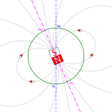
The variation between magnetic north (N
m) and "true" north (N
g).
Near the surface of the Earth, its magnetic field can be closely approximated by the field of a
magnetic dipole positioned at the center of the Earth and tilted at an angle of about 10° with respect to the
rotational axis of the Earth.
[13] The dipole is roughly equivalent to a powerful bar
magnet, with its south pole pointing towards the
geomagnetic North Pole.
[16] This may seem surprising, but the north pole of a magnet is so defined because, if allowed to rotate freely, it points roughly northward (in the geographic sense). Since the north pole of a magnet attracts the south poles of other magnets and repels the north poles, it must be attracted to the south pole of Earth's magnet. The dipolar field accounts for 80–90% of the field in most locations.
[12]
Magnetic poles

The movement of Earth's North Magnetic Pole across the Canadian arctic, 1831–2007.
The positions of the magnetic poles can be defined in at least two ways: locally or globally.
[17]
One way to define a pole is as a point where the magnetic field is vertical.
[18] This can be determined by measuring the inclination, as described above. The inclination of the Earth's field is 90° (upwards) at the
North Magnetic Pole and -90°(downwards) at the
South Magnetic Pole. The two poles wander independently of each other and are not directly opposite each other on the globe. They can migrate rapidly: movements of up to 40 kilometres (25 mi) per year have been observed for the North Magnetic Pole. Over the last 180 years, the North Magnetic Pole has been migrating northwestward, from Cape Adelaide in the
Boothia Peninsula in 1831 to 600 kilometres (370 mi) from
Resolute Bay in 2001.
[19] The
magnetic equator is the line where the inclination is zero (the magnetic field is horizontal).
The global definition of the Earth's field is based on a mathematical model. If a line is drawn through the center of the Earth, parallel to the moment of the best-fitting magnetic dipole, the two positions where it intersects the Earth's surface are called the North and South
geomagnetic poles. If the Earth's magnetic field were perfectly dipolar, the geomagnetic poles and magnetic dip poles would coincide and compasses would point towards them. However, the Earth's field has a significant
non-dipolar contribution, so the poles do not coincide and compasses do not generally point at either.
Magnetosphere
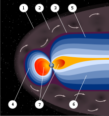
An artist's rendering of the structure of a magnetosphere. 1) Bow shock. 2) Magnetosheath. 3) Magnetopause. 4) Magnetosphere. 5) Northern tail lobe. 6) Southern tail lobe. 7) Plasmasphere.
Earth's magnetic field, predominantly dipolar at its surface, is distorted further out by the
solar wind. This is a stream of charged particles leaving the Sun's
corona and accelerating to a speed of 200 to 1000 kilometres per second. They carry with them a magnetic field, the
interplanetary magnetic field (IMF).
[20]
The solar wind exerts a pressure, and if it could reach Earth's atmosphere it would erode it. However, it is kept away by the pressure of the Earth's magnetic field. The
magnetopause, the area where the pressures balance, is the boundary of the
magnetosphere. Despite its name, the magnetosphere is asymmetric, with the sunward side being about 10
Earth radii out but the other side stretching out in a
magnetotail that extends beyond 200 Earth radii.
[21] Sunward of the magnetopause is the
bow shock, the area where the solar wind slows abruptly.
[20]
Inside the magnetosphere is the
plasmasphere, a donut-shaped region containing low-energy charged particles, or
plasma. This region begins at a height of 60 km, extends up to 3 or 4 Earth radii, and includes the
ionosphere. This region rotates with the Earth.
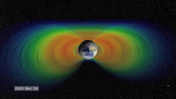
[21] There are also two concentric tire-shaped regions, called the
Van Allen radiation belts, with high-energy ions (energies from 0.1 to 10 million
electron volts (MeV)). The inner belt is 1–2 Earth radii out while the outer belt is at 4–7 Earth radii. The plasmasphere and Van Allen belts have partial overlap, with the extent of overlap varying greatly with solar activity.
[22]
As well as deflecting the solar wind, the Earth's magnetic field deflects
cosmic rays, high-energy charged particles that are mostly from outside the
Solar system. (Many cosmic rays are kept out of the Solar system by the Sun's magnetosphere, or
heliosphere.
[23]) By contrast, astronauts on the Moon risk exposure to radiation. Anyone who had been on the Moon's surface during a particularly violent solar eruption in 2005 would have received a lethal dose.
[20]
Some of the charged particles do get into the magnetosphere. These spiral around field lines, bouncing back and forth between the poles several times per second. In addition, positive ions slowly drift westward and negative ions drift eastward, giving rise to a
ring current. This current reduces the magnetic field at the Earth's surface.
[20] Particles that penetrate the ionosphere and collide with the atoms there give rise to the lights of the
aurorae and also emit
X-rays.
[21]
The varying conditions in the magnetosphere, known as
space weather, are largely driven by solar activity. If the solar wind is weak, the magnetosphere expands; while if it is strong, it compresses the magnetosphere and more of it gets in. Periods of particularly intense activity, called
geomagnetic storms, can occur when a
coronal mass ejection erupts above the Sun and sends a shock wave through the Solar System. Such a wave can take just two days to reach the Earth. Geomagnetic storms can cause a lot of disruption;
the "Halloween" storm of 2003 damaged more than a third of NASA's satellites. The largest documented storm occurred in 1859. It induced currents strong enough to short out telegraph lines, and aurorae were reported as far south as Hawaii.
[20][24]
Time dependence
Short-term variations
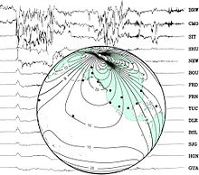
Background: a set of traces from magnetic observatories showing a
magnetic storm in 2000.
Globe: map showing locations of observatories and contour lines giving horizontal magnetic intensity in
μ T.
The geomagnetic field changes on time scales from milliseconds to millions of years. Shorter time scales mostly arise from currents in the
ionosphere (
ionospheric dynamo region) and
magnetosphere, and some changes can be traced to
geomagnetic storms or daily variations in currents. Changes over time scales of a year or more mostly reflect changes in the
Earth's interior, particularly the iron-rich
core.
[12]
Frequently, the Earth's
magnetosphere is hit by
solar flares causing
geomagnetic storms, provoking displays of
aurorae. The short-term instability of the magnetic field is measured with the
K-index.
[25]
Data from
THEMIS show that the magnetic field, which interacts with the
solar wind, is reduced when the magnetic orientation is aligned between Sun and Earth - opposite to the previous hypothesis. During forthcoming
solar storms, this could result in
blackouts and disruptions in
artificial satellites.
[26]
Secular variation
Estimated declination contours by year, 1590 to 1990 (click to see variation).
Changes in Earth's magnetic field on a time scale of a year or more are referred to as
secular variation. Over hundreds of years,
magnetic declination is observed to vary over tens of degrees.
[12] A movie on the right shows how global declinations have changed over the last few centuries.
[27]
The direction and intensity of the dipole change over time. Over the last two centuries the dipole strength has been decreasing at a rate of about 6.3% per century.
[12] At this rate of decrease, the field would be negligible in about 1600 years.
[28] However, this strength is about average for the last 7 thousand years, and the current rate of change is not unusual.
[29]
A prominent feature in the non-dipolar part of the secular variation is a
westward drift at a rate of about 0.2 degrees per year.
[28] This drift is not the same everywhere and has varied over time. The globally averaged drift has been westward since about 1400 AD but eastward between about 1000 AD and 1400 AD.
[30]
Changes that predate magnetic observatories are recorded in archaeological and geological materials. Such changes are referred to as
paleomagnetic secular variation or
paleosecular variation (PSV). The records typically include long periods of small change with occasional large changes reflecting
geomagnetic excursions and reversals.
[31]
Magnetic field reversals

Geomagnetic polarity during the late
Cenozoic Era. Dark areas denote periods where the polarity matches today's polarity, light areas denote periods where that polarity is reversed.
Although generally Earth's field is approximately dipolar and its magnetic moment is nearly aligned with the rotational axis, occasionally the North and South
geomagnetic poles trade places. Evidence for these
geomagnetic reversals can be found worldwide in
basalts, sediment cores taken from the ocean floors, and seafloor magnetic anomalies.
[32] Reversals occur at apparently random intervals ranging from less than 0.1 million years to as much as 50 million years. The most recent geomagnetic reversal, called the
Brunhes–Matuyama reversal, occurred about 780,000 years ago.
[19][33] Another global reversal of the Earth's field, called the
Laschamp event, occurred during the last ice age (41,000 years ago). However, because of its brief duration it is labelled an
excursion.
[34][35]
The past magnetic field is recorded mostly by
strongly magnetic minerals, particularly
iron oxides such as
magnetite, that can carry a permanent magnetic moment. This
remanent magnetization, or
remanence, can be acquired in more than one way. In
lava flows, the direction of the field is "frozen" in small minerals as they cool, giving rise to a
thermoremanent magnetization. In sediments, the orientation of magnetic particles acquires a slight bias towards the magnetic field as they are deposited on an ocean floor or lake bottom. This is called
detrital remanent magnetization.
[8]
Thermoremanent magnetization is the main source of the magnetic anomalies around
ocean ridges. As the seafloor spreads,
magma wells up from the
mantle, cools to form new basaltic crust on both sides of the ridge, and is carried away from it by
seafloor spreading. As it cools, it records the direction of the Earth's field. When the Earth's field reverses, new basalt records the reversed direction. The result is a series of stripes that are symmetric about the ridge. A ship towing a magnetometer on the surface of the ocean can detect these stripes and infer the age of the ocean floor below. This provides information on the rate at which seafloor has spread in the past.
[8]
Radiometric dating of lava flows has been used to establish a
geomagnetic polarity time scale, part of which is shown in the image. This forms the basis of
magnetostratigraphy, a geophysical correlation technique that can be used to date both sedimentary and volcanic sequences as well as the seafloor magnetic anomalies.
[8]
Studies of lava flows on
Steens Mountain, Oregon, indicate that the magnetic field could have shifted at a rate of up to 6 degrees per day at some time in Earth's history, which significantly challenges the popular understanding of how the Earth's magnetic field works.
[36]
Temporary dipole tilt variations that take the dipole axis across the equator and then back to the original polarity are known as
excursions.
[35]
Earliest appearance
A paleomagnetic study of Australian red dacite and
pillow basalt has estimated the magnetic field to have been present since at least
3,450 million years ago.
[37][38][39]
Future

Variations in virtual axial dipole moment since the last reversal.
At present, the overall geomagnetic field is becoming weaker; the present strong deterioration corresponds to a 10–15% decline over the last 150 years and has accelerated in the past several years; geomagnetic intensity has declined almost continuously from a maximum 35% above the modern value achieved approximately 2,000 years ago. The rate of decrease and the current strength are within the normal range of variation, as shown by the record of past magnetic fields recorded in rocks (figure on right).
The nature of Earth's magnetic field is one of
heteroscedastic fluctuation. An instantaneous measurement of it, or several measurements of it across the span of decades or centuries, are not sufficient to extrapolate an overall trend in the field strength. It has gone up and down in the past for no apparent reason. Also, noting the local intensity of the dipole field (or its fluctuation) is insufficient to characterize Earth's magnetic field as a whole, as it is not strictly a dipole field. The dipole component of Earth's field can diminish even while the total magnetic field remains the same or increases.
The Earth's
magnetic north pole is drifting from northern
Canada towards
Siberia with a presently accelerating rate—10 kilometres (6.2 mi) per year at the beginning of the 20th century, up to 40 kilometres (25 mi) per year in 2003,
[19] and since then has only accelerated.
[40]
Physical origin
The Earth's magnetic field is believed to be generated by electric currents in the conductive material of its core, created by
convection currents due to heat escaping from the core. However the process is complex, and computer models that reproduce some of its features have only been developed in the last few decades.
Earth's core and the geodynamo

A schematic illustrating the relationship between motion of conducting fluid, organized into rolls by the Coriolis force, and the magnetic field the motion generates.
[41]
The Earth and most of the planets in the Solar System, as well as the Sun and other stars, all generate magnetic fields through the motion of highly
conductive fluids.
[42] The Earth's field originates in its core. This is a region of iron alloys extending to about 3400 km (the radius of the Earth is 6370 km). It is divided into a solid
inner core, with a radius of 1220 km, and a liquid
outer core.
[43] The motion of the liquid in the outer core is driven by heat flow from the inner core, which is about 6,000 K (5,730 °C; 10,340 °F), to the
core-mantle boundary, which is about 3,800 K (3,530 °C; 6,380 °F).
[44] The pattern of flow is organized by the rotation of the Earth and the presence of the solid inner core.
[45]
The mechanism by which the Earth generates a magnetic field is known as a
dynamo.
[42] A magnetic field is generated by a feedback loop: current loops generate magnetic fields (
Ampère's circuital law); a changing magnetic field generates an electric field (
Faraday's law); and the electric and magnetic fields exert a force on the charges that are flowing in currents (the
Lorentz force).
[46] These effects can be combined in a
partial differential equation for the magnetic field called the
magnetic induction equation:

...where
u is the velocity of the fluid;
B is the
magnetic B-field; and
η=1/σμ is the
magnetic diffusivity, which is inversely proportional to the product of the
electrical conductivity σ and the
permeability μ .
[47] The term
∂B/∂t is the time derivative of the field;
∇2 is the
Laplace operator and
∇× is the
curl operator.
The first term on the right hand side of the induction equation is a
diffusion term. In a stationary fluid, the magnetic field declines and any concentrations of field spread out. If the Earth's dynamo shut off, the dipole part would disappear in a few tens of thousands of years.
[47]
In a perfect conductor (
σ=∞), there would be no diffusion. By
Lenz's law, any change in the magnetic field would be immediately opposed by currents, so the flux through a given volume of fluid could not change. As the fluid moved, the magnetic field would go with it. The theorem describing this effect is called the
frozen-in-field theorem. Even in a fluid with a finite conductivity, new field is generated by stretching field lines as the fluid moves in ways that deform it. This process could go on generating new field indefinitely, were it not that as the magnetic field increases in strength, it resists fluid motion.
[47]
The motion of the fluid is sustained by
convection, motion driven by
buoyancy. The temperature increases towards the center of the Earth, and the higher temperature of the fluid lower down makes it buoyant. This buoyancy is enhanced by chemical separation: As the core cools, some of the molten iron solidifies and is plated to the
inner core. In the process, lighter elements are left behind in the fluid, making it lighter. This is called
compositional convection. A
Coriolis effect, caused by the overall planetary rotation, tends to organize the flow into rolls aligned along the north-south polar axis.
[45][47]
Given a magnetic field, a dynamo can make it grow, but it needs a "seed" field to get it started.
[47] For the Earth, this could have been an external magnetic field. Early in its history the Sun went through a
T-Tauri phase in which the
solar wind would have had a magnetic field orders of magnitude larger than the present solar wind.
[48] However, much of the field may have been screened out by the Earth's mantle. An alternative source is currents in the core-mantle boundary driven by chemical reactions or variations in thermal or electric conductivity. Such effects may still provide a small bias that are part of the boundary conditions for the geodynamo.
[49]
The average magnetic field in the Earth's outer core was calculated to be 25
gauss, 50 times stronger than the field at the surface.
[50]
Numerical models
Simulating the geodynamo requires numerically solving a set of nonlinear partial differential equations for the
magnetohydrodynamics (MHD) of the Earth's interior. Simulation of the MHD equations is performed on a 3D grid of points and the fineness of the grid, which in part determines the realism of the solutions, is limited mainly by computer power. For decades, theorists were confined to creating
kinematic dynamos in which the fluid motion is chosen in advance and the effect on the magnetic field calculated. Kinematic dynamo theory was mainly a matter of trying different flow geometries and testing whether such geometries could sustain a dynamo.
[51]
The first
self-consistent dynamo models, ones that determine both the fluid motions and the magnetic field, were developed by two groups in 1995, one in Japan
[52] and one in the United States.
[1][53] The latter received attention because it successfully reproduced some of the characteristics of the Earth's field, including geomagnetic reversals.
[51]
Currents in the ionosphere and magnetosphere
Electric currents induced in the
ionosphere generate magnetic fields (
ionospheric dynamo region). Such a field is always generated near where the atmosphere is closest to the Sun, causing daily alterations that can deflect surface magnetic fields by as much as one degree. Typical daily variations of field strength are about 25 nanoteslas (nT) (one part in 2000), with variations over a few seconds of typically around 1 nT (one part in 50,000).
[54]
Measurement and analysis
Detection
The Earth's magnetic field strength was measured by
Carl Friedrich Gauss in 1835 and has been repeatedly measured since then, showing a relative decay of about 10% over the last 150 years.
[55] The
Magsat satellite and later satellites have used 3-axis vector magnetometers to probe the 3-D structure of the Earth's magnetic field. The later
Ørsted satellite allowed a comparison indicating a dynamic geodynamo in action that appears to be giving rise to an alternate pole under the Atlantic Ocean west of S. Africa.
[56]
Governments sometimes operate units that specialize in measurement of the Earth's magnetic field. These are
geomagnetic observatories, typically part of a national
Geological survey, for example the
British Geological Survey's
Eskdalemuir Observatory. Such observatories can measure and forecast magnetic conditions such as magnetic storms that sometimes affect communications, electric power, and other human activities.
The
International Real-time Magnetic Observatory Network, with over 100 interlinked geomagnetic observatories around the world has been recording the earths magnetic field since 1991.
The military determines local geomagnetic field characteristics, in order to detect
anomalies in the natural background that might be caused by a significant metallic object such as a submerged submarine. Typically, these
magnetic anomaly detectors are flown in aircraft like the UK's
Nimrod or towed as an instrument or an array of instruments from surface ships.
Commercially,
geophysical prospecting companies also use magnetic detectors to identify naturally occurring anomalies from
ore bodies, such as the
Kursk Magnetic Anomaly.
Crustal magnetic anomalies

A model of short-wavelength features of Earth's magnetic field, attributed to lithospheric anomalies.
[57]
Magnetometers detect minute deviations in the Earth's magnetic field caused by iron
artifacts, kilns, some types of stone structures, and even ditches and
middens in
archaeological geophysics. Using magnetic instruments adapted from airborne
magnetic anomaly detectors developed during World War II to detect submarines, the magnetic variations across the ocean floor have been mapped.
Basalt — the iron-rich, volcanic rock making up the ocean floor — contains a strongly magnetic mineral (
magnetite) and can locally distort compass readings. The distortion was recognized by Icelandic mariners as early as the late 18th century. More important, because the presence of magnetite gives the basalt measurable magnetic properties, these magnetic variations have provided another means to study the deep ocean floor. When newly formed rock cools, such magnetic materials record the Earth's magnetic field.
Statistical models
Each measurement of the magnetic field is at a particular place and time. If an accurate estimate of the field at some other place and time is needed, the measurements must be converted to a model and the model used to make predictions.
Spherical harmonics

Schematic representation of spherical harmonics on a sphere and their nodal lines.
Pℓ m is equal to 0 along
m great circles passing through the poles, and along
ℓ-m circles of equal latitude. The function changes sign each ℓtime it crosses one of these lines.
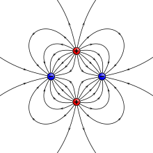
Example of a quadrupole field. This could also be constructed by moving two dipoles together. If this arrangement were placed at the center of the Earth, then a magnetic survey at the surface would find two magnetic north poles (at the geographic poles) and two south poles at the equator.
The most common way of analyzing the global variations in the Earth's magnetic field is to fit the measurements to a set of
spherical harmonics. This was first done by
Carl Friedrich Gauss.
[58] Spherical harmonics are functions that oscillate over the surface of a sphere. They are the product of two functions, one that depends on latitude and one on longitude. The function of longitude is zero along zero or more great circles passing through the North and South Poles; the number of such
nodal lines is the absolute value of the
order m. The function of latitude is zero along zero or more latitude circles; this plus the order is equal to the
degree ℓ. Each harmonic is equivalent to a particular arrangement of magnetic charges at the center of the Earth. A
monopole is an isolated magnetic charge, which has never been observed. A
dipole is equivalent to two opposing charges brought close together and a
quadrupole to two dipoles brought together. A quadrupole field is shown in the lower figure on the right.
[12]
Spherical harmonics can represent any
scalar field (function of position) that satisfies certain properties. A magnetic field is a
vector field, but if it is expressed in Cartesian components
X, Y, Z, each component is the derivative of the same scalar function called the
magnetic potential. Analyses of the Earth's magnetic field use a modified version of the usual spherical harmonics that differ by a multiplicative factor. A least-squares fit to the magnetic field measurements gives the Earth's field as the sum of spherical harmonics, each multiplied by the best-fitting
Gauss coefficient gmℓ or
hmℓ.
[12]
The lowest-degree Gauss coefficient,
g00, gives the contribution of an isolated magnetic charge, so it is zero. The next three coefficients –
g10,
g11, and
h11 – determine the direction and magnitude of the dipole contribution. The best fitting dipole is tilted at an angle of about 10° with respect to the rotational axis, as described earlier.
[12]
Radial dependence
Spherical harmonic analysis can be used to distinguish internal from external sources if measurements are available at more than one height (for example, ground observatories and satellites). In that case, each term with coefficient
gmℓ or
hmℓ can be split into two terms: one that decreases with radius as
1/rℓ+1 and one that
increases with radius as
rℓ. The increasing terms fit the external sources (currents in the ionosphere and magnetosphere). However, averaged over a few years the external contributions average to zero.
[12]
The remaining terms predict that the potential of a dipole source (
ℓ=1) drops off as
1/r2. The magnetic field, being a derivative of the potential, drops off as
1/r3. Quadrupole terms drop off as
1/r4, and higher order terms drop off increasingly rapidly with the radius. The radius of the
outer core is about half of the radius of the Earth. If the field at the core-mantle boundary is fit to spherical harmonics, the dipole part is smaller by a factor of about 8 at the surface, the quadrupole part by a factor of 16, and so on. Thus, only the components with large wavelengths can be noticeable at the surface. From a variety of arguments, it is usually assumed that only terms up to degree
14 or less have their origin in the core. These have wavelengths of about 2,000 kilometres (1,200 mi) or less. Smaller features are attributed to crustal anomalies.
[12]
Global models
The
International Association of Geomagnetism and Aeronomy maintains a standard global field model called the
International Geomagnetic Reference Field. It is updated every 5 years. The 11th-generation model, IGRF11, was developed using data from satellites (
Ørsted,
CHAMP and
SAC-C) and a world network of geomagnetic observatories.
[59] The spherical harmonic expansion was truncated at degree 10, with 120 coefficients, until 2000. Subsequent models are truncated at degree 13 (195 coefficients).
[60]
Another global field model, called
World Magnetic Model, is produced jointly by the National Geophysical Data Center and the
British Geological Survey. This model truncates at degree 12 (168 coefficients). It is the model used by the
United States Department of Defense, the
Ministry of Defence (United Kingdom), the
North Atlantic Treaty Organization, and the
International Hydrographic Office as well as in many civilian navigation systems.
[61]
A third model, produced by the
Goddard Space Flight Center (
NASA and
GSFC) and the
Danish Space Research Institute, uses a "comprehensive modeling" approach that attempts to reconcile data with greatly varying temporal and spatial resolution from ground and satellite sources.
[62]
Biomagnetism
Animals including birds and turtles can detect the Earth's magnetic field, and use the field to navigate during
migration.
[63] Cows and wild deer tend to align their bodies north-south while relaxing, but not when the animals are under
high voltage power lines[clarify], leading researchers to believe magnetism is responsible.
[64][65] In 2011 a group of
Czech researchers reported their failed attempt to replicate the finding using different
Google Earth images.
[66]
Researchers found out that very weak electromagnetic fields disrupt the magnetic compass used by European robins and other songbirds to navigate using the Earth's magnetic field. Neither power lines nor cellphone signals are to blame for the electromagnetic field effect on the birds, according to the new study published in the 8 May 2014 edition of the journal Nature. Instead, the culprits consist of frequencies between 2 kHz and 5 MHz, such as AM radio signals and ordinary electronic equipment that might be found in businesses or private homes.
[67]


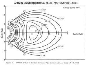 AP8 MIN omnidirectional proton flux ≥ 100 keV
 AP8 MIN omnidirectional proton flux ≥ 1 MeV
 AP8 MIN omnidirectional proton flux ≥ 400 MeV