Population genetics

From Wikipedia, the free encyclopedia

https://en.wikipedia.org/wiki/Population_genetics 

Population genetics is a subfield of genetics that deals with genetic differences within and between populations, and is a part of evolutionary biology. Studies in this branch of biology examine such phenomena as adaptation, speciation, and population structure.

Population genetics was a vital ingredient in the emergence of the modern evolutionary synthesis. Its primary founders were Sewall Wright, J. B. S. Haldane and Ronald Fisher, who also laid the foundations for the related discipline of quantitative genetics. Traditionally a highly mathematical discipline, modern population genetics encompasses theoretical, laboratory, and field work. Population genetic models are used both for statistical inference from DNA sequence data and for proof/disproof of concept.

What sets population genetics apart from newer, more phenotypic approaches to modelling evolution, such as evolutionary game theory and adaptive dynamics, is its emphasis on such genetic phenomena as dominance, epistasis, the degree to which genetic recombination breaks linkage disequilibrium, and the random phenomena of mutation and genetic drift. This makes it appropriate for comparison to population genomics data.

History

Population genetics began as a reconciliation of Mendelian inheritance and biostatistics models. Natural selection will only cause evolution if there is enough genetic variation in a population. Before the discovery of Mendelian genetics, one common hypothesis was blending inheritance. But with blending inheritance, genetic variance would be rapidly lost, making evolution by natural or sexual selection implausible. The Hardy–Weinberg principle provides the solution to how variation is maintained in a population with Mendelian inheritance. According to this principle, the frequencies of alleles (variations in a gene) will remain constant in the absence of selection, mutation, migration and genetic drift.

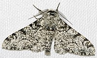
The typical white-bodied form of the peppered moth.

 

Industrial melanism: the black-bodied form of the peppered moth appeared in polluted areas.

The next key step was the work of the British biologist and statistician Ronald Fisher. In a series of papers starting in 1918 and culminating in his 1930 book The Genetical Theory of Natural Selection, Fisher showed that the continuous variation measured by the biometricians could be produced by the combined action of many discrete genes, and that natural selection could change allele frequencies in a population, resulting in evolution. In a series of papers beginning in 1924, another British geneticist, J. B. S. Haldane, worked out the mathematics of allele frequency change at a single gene locus under a broad range of conditions. Haldane also applied statistical analysis to real-world examples of natural selection, such as peppered moth evolution and industrial melanism, and showed that selection coefficients could be larger than Fisher assumed, leading to more rapid adaptive evolution as a camouflage strategy following increased pollution.

The American biologist Sewall Wright, who had a background in animal breeding experiments, focused on combinations of interacting genes, and the effects of inbreeding on small, relatively isolated populations that exhibited genetic drift. In 1932 Wright introduced the concept of an adaptive landscape and argued that genetic drift and inbreeding could drive a small, isolated sub-population away from an adaptive peak, allowing natural selection to drive it towards different adaptive peaks.

The work of Fisher, Haldane and Wright founded the discipline of population genetics. This integrated natural selection with Mendelian genetics, which was the critical first step in developing a unified theory of how evolution worked. John Maynard Smith was Haldane's pupil, whilst W. D. Hamilton was influenced by the writings of Fisher. The American George R. Price worked with both Hamilton and Maynard Smith. American Richard Lewontin and Japanese Motoo Kimura were influenced by Wright and Haldane.

Gertrude Hauser and Heidi Danker–Hopfe have suggested that Hubert Walter also contributed to the creation of the subdiscipline population genetics.

Modern synthesis

The mathematics of population genetics were originally developed as the beginning of the modern synthesis. Authors such as Beatty have asserted that population genetics defines the core of the modern synthesis. For the first few decades of the 20th century, most field naturalists continued to believe that Lamarckism and orthogenesis provided the best explanation for the complexity they observed in the living world. During the modern synthesis, these ideas were purged, and only evolutionary causes that could be expressed in the mathematical framework of population genetics were retained. Consensus was reached as to which evolutionary factors might influence evolution, but not as to the relative importance of the various factors.

Theodosius Dobzhansky, a postdoctoral worker in T. H. Morgan's lab, had been influenced by the work on genetic diversity by Russian geneticists such as Sergei Chetverikov. He helped to bridge the divide between the foundations of microevolution developed by the population geneticists and the patterns of macroevolution observed by field biologists, with his 1937 book Genetics and the Origin of Species. Dobzhansky examined the genetic diversity of wild populations and showed that, contrary to the assumptions of the population geneticists, these populations had large amounts of genetic diversity, with marked differences between sub-populations. The book also took the highly mathematical work of the population geneticists and put it into a more accessible form. Many more biologists were influenced by population genetics via Dobzhansky than were able to read the highly mathematical works in the original.

In Great Britain E. B. Ford, the pioneer of ecological genetics, continued throughout the 1930s and 1940s to empirically demonstrate the power of selection due to ecological factors including the ability to maintain genetic diversity through genetic polymorphisms such as human blood types. Ford's work, in collaboration with Fisher, contributed to a shift in emphasis during the modern synthesis towards natural selection as the dominant force.

Neutral theory and origin-fixation dynamics

The original, modern synthesis view of population genetics assumes that mutations provide ample raw material, and focuses only on the change in frequency of alleles within populations. The main processes influencing allele frequencies are natural selection, genetic drift, gene flow and recurrent mutation. Fisher and Wright had some fundamental disagreements about the relative roles of selection and drift. The availability of molecular data on all genetic differences led to the neutral theory of molecular evolution. In this view, many mutations are deleterious and so never observed, and most of the remainder are neutral, i.e. are not under selection. With the fate of each neutral mutation left to chance (genetic drift), the direction of evolutionary change is driven by which mutations occur, and so cannot be captured by models of change in the frequency of (existing) alleles alone.

The origin-fixation view of population genetics generalizes this approach beyond strictly neutral mutations, and sees the rate at which a particular change happens as the product of the mutation rate and the fixation probability.

Four processes

Selection

Natural selection, which includes sexual selection, is the fact that some traits make it more likely for an organism to survive and reproduce. Population genetics describes natural selection by defining fitness as a propensity or probability of survival and reproduction in a particular environment. The fitness is normally given by the symbol w=1-s where s is the selection coefficient. Natural selection acts on phenotypes, so population genetic models assume relatively simple relationships to predict the phenotype and hence fitness from the allele at one or a small number of loci. In this way, natural selection converts differences in the fitness of individuals with different phenotypes into changes in allele frequency in a population over successive generations.

Before the advent of population genetics, many biologists doubted that small differences in fitness were sufficient to make a large difference to evolution. Population geneticists addressed this concern in part by comparing selection to genetic drift. Selection can overcome genetic drift when s is greater than 1 divided by the effective population size. When this criterion is met, the probability that a new advantageous mutant becomes fixed is approximately equal to 2s. The time until fixation of such an allele depends little on genetic drift, and is approximately proportional to log(sN)/s.

Dominance

Dominance means that the phenotypic and/or fitness effect of one allele at a locus depends on which allele is present in the second copy for that locus. Consider three genotypes at one locus, with the following fitness values

Genotype:	A1A1	A1A2	A2A2
Relative fitness:	1	1-hs	1-s

s is the selection coefficient and h is the dominance coefficient. The value of h yields the following information:

h=0	A1 dominant, A2 recessive
h=1	A2 dominant, A1 recessive
0<h<1	incomplete dominance
h<0	overdominance
h>1	Underdominance

Epistasis

The logarithm of fitness as a function of the number of deleterious mutations. Synergistic epistasis is represented by the red line - each subsequent deleterious mutation has a larger proportionate effect on the organism's fitness. Antagonistic epistasis is in blue. The black line shows the non-epistatic case, where fitness is the product of the contributions from each of its loci.

Epistasis means that the phenotypic and/or fitness effect of an allele at one locus depends on which alleles are present at other loci. Selection does not act on a single locus, but on a phenotype that arises through development from a complete genotype. However, many population genetics models of sexual species are "single locus" models, where the fitness of an individual is calculated as the product of the contributions from each of its loci—effectively assuming no epistasis.

In fact, the genotype to fitness landscape is more complex. Population genetics must either model this complexity in detail, or capture it by some simpler average rule. Empirically, beneficial mutations tend to have a smaller fitness benefit when added to a genetic background that already has high fitness: this is known as diminishing returns epistasis. When deleterious mutations also have a smaller fitness effect on high fitness backgrounds, this is known as "synergistic epistasis". However, the effect of deleterious mutations tends on average to be very close to multiplicative, or can even show the opposite pattern, known as "antagonistic epistasis".

Synergistic epistasis is central to some theories of the purging of mutation load and to the evolution of sexual reproduction.

Mutation

Drosophila melanogaster

Mutation is the ultimate source of genetic variation in the form of new alleles. In addition, mutation may influence the direction of evolution when there is mutation bias, i.e. different probabilities for different mutations to occur. For example, recurrent mutation that tends to be in the opposite direction to selection can lead to mutation–selection balance. At the molecular level, if mutation from G to A happens more often than mutation from A to G, then genotypes with A will tend to evolve. Different insertion vs. deletion mutation biases in different taxa can lead to the evolution of different genome sizes. Developmental or mutational biases have also been observed in morphological evolution. For example, according to the phenotype-first theory of evolution, mutations can eventually cause the genetic assimilation of traits that were previously induced by the environment.

Mutation bias effects are superimposed on other processes. If selection would favor either one out of two mutations, but there is no extra advantage to having both, then the mutation that occurs the most frequently is the one that is most likely to become fixed in a population.

Mutation can have no effect, alter the product of a gene, or prevent the gene from functioning. Studies in the fly Drosophila melanogaster suggest that if a mutation changes a protein produced by a gene, this will probably be harmful, with about 70 percent of these mutations having damaging effects, and the remainder being either neutral or weakly beneficial. Most loss of function mutations are selected against. But when selection is weak, mutation bias towards loss of function can affect evolution. For example, pigments are no longer useful when animals live in the darkness of caves, and tend to be lost. This kind of loss of function can occur because of mutation bias, and/or because the function had a cost, and once the benefit of the function disappeared, natural selection leads to the loss. Loss of sporulation ability in a bacterium during laboratory evolution appears to have been caused by mutation bias, rather than natural selection against the cost of maintaining sporulation ability. When there is no selection for loss of function, the speed at which loss evolves depends more on the mutation rate than it does on the effective population size, indicating that it is driven more by mutation bias than by genetic drift.

Mutations can involve large sections of DNA becoming duplicated, usually through genetic recombination. This leads to copy-number variation within a population. Duplications are a major source of raw material for evolving new genes. Other types of mutation occasionally create new genes from previously noncoding DNA.

Genetic drift

Genetic drift is a change in allele frequencies caused by random sampling. That is, the alleles in the offspring are a random sample of those in the parents. Genetic drift may cause gene variants to disappear completely, and thereby reduce genetic variability. In contrast to natural selection, which makes gene variants more common or less common depending on their reproductive success, the changes due to genetic drift are not driven by environmental or adaptive pressures, and are equally likely to make an allele more common as less common.

The effect of genetic drift is larger for alleles present in few copies than when an allele is present in many copies. The population genetics of genetic drift are described using either branching processes or a diffusion equation describing changes in allele frequency. These approaches are usually applied to the Wright-Fisher and Moran models of population genetics. Assuming genetic drift is the only evolutionary force acting on an allele, after t generations in many replicated populations, starting with allele frequencies of p and q, the variance in allele frequency across those populations is

${\displaystyle V_{t}\approx pq\left(1-\exp \left\{-{\frac {t}{2N_{e}}}\right\}\right).}$

Ronald Fisher held the view that genetic drift plays at the most a minor role in evolution, and this remained the dominant view for several decades. No population genetics perspective have ever given genetic drift a central role by itself, but some have made genetic drift important in combination with another non-selective force. The shifting balance theory of Sewall Wright held that the combination of population structure and genetic drift was important. Motoo Kimura's neutral theory of molecular evolution claims that most genetic differences within and between populations are caused by the combination of neutral mutations and genetic drift.

The role of genetic drift by means of sampling error in evolution has been criticized by John H Gillespie and Will Provine, who argue that selection on linked sites is a more important stochastic force, doing the work traditionally ascribed to genetic drift by means of sampling error. The mathematical properties of genetic draft are different from those of genetic drift. The direction of the random change in allele frequency is autocorrelated across generations.

Gene flow

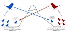
Gene flow is the transfer of alleles from one population to another population through immigration of individuals. In this example, one of the birds from population A immigrates to population B, which has fewer of the dominant alleles, and through mating incorporates its alleles into the other population.

Because of physical barriers to migration, along with the limited tendency for individuals to move or spread (vagility), and tendency to remain or come back to natal place (philopatry), natural populations rarely all interbreed as may be assumed in theoretical random models (panmixy). There is usually a geographic range within which individuals are more closely related to one another than those randomly selected from the general population. This is described as the extent to which a population is genetically structured.

The Great Wall of China is an obstacle to gene flow of some terrestrial species.

Genetic structuring can be caused by migration due to historical climate change, species range expansion or current availability of habitat. Gene flow is hindered by mountain ranges, oceans and deserts or even man-made structures such as the Great Wall of China, which has hindered the flow of plant genes.

Gene flow is the exchange of genes between populations or species, breaking down the structure. Examples of gene flow within a species include the migration and then breeding of organisms, or the exchange of pollen. Gene transfer between species includes the formation of hybrid organisms and horizontal gene transfer. Population genetic models can be used to identify which populations show significant genetic isolation from one another, and to reconstruct their history.

Subjecting a population to isolation leads to inbreeding depression. Migration into a population can introduce new genetic variants, potentially contributing to evolutionary rescue. If a significant proportion of individuals or gametes migrate, it can also change allele frequencies, e.g. giving rise to migration load.

In the presence of gene flow, other barriers to hybridization between two diverging populations of an outcrossing species are required for the populations to become new species.

Horizontal gene transfer

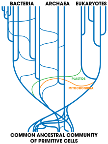
Current tree of life showing vertical and horizontal gene transfers.

Horizontal gene transfer is the transfer of genetic material from one organism to another organism that is not its offspring; this is most common among prokaryotes. In medicine, this contributes to the spread of antibiotic resistance, as when one bacteria acquires resistance genes it can rapidly transfer them to other species. Horizontal transfer of genes from bacteria to eukaryotes such as the yeast Saccharomyces cerevisiae and the adzuki bean beetle Callosobruchus chinensis may also have occurred. An example of larger-scale transfers are the eukaryotic bdelloid rotifers, which appear to have received a range of genes from bacteria, fungi, and plants. Viruses can also carry DNA between organisms, allowing transfer of genes even across biological domains. Large-scale gene transfer has also occurred between the ancestors of eukaryotic cells and prokaryotes, during the acquisition of chloroplasts and mitochondria.

Linkage

If all genes are in linkage equilibrium, the effect of an allele at one locus can be averaged across the gene pool at other loci. In reality, one allele is frequently found in linkage disequilibrium with genes at other loci, especially with genes located nearby on the same chromosome. Recombination breaks up this linkage disequilibrium too slowly to avoid genetic hitchhiking, where an allele at one locus rises to high frequency because it is linked to an allele under selection at a nearby locus. Linkage also slows down the rate of adaptation, even in sexual populations. The effect of linkage disequilibrium in slowing down the rate of adaptive evolution arises from a combination of the Hill–Robertson effect (delays in bringing beneficial mutations together) and background selection (delays in separating beneficial mutations from deleterious hitchhikers).

Linkage is a problem for population genetic models that treat one gene locus at a time. It can, however, be exploited as a method for detecting the action of natural selection via selective sweeps.

In the extreme case of an asexual population, linkage is complete, and population genetic equations can be derived and solved in terms of a travelling wave of genotype frequencies along a simple fitness landscape. Most microbes, such as bacteria, are asexual. The population genetics of their adaptation have two contrasting regimes. When the product of the beneficial mutation rate and population size is small, asexual populations follow a "successional regime" of origin-fixation dynamics, with adaptation rate strongly dependent on this product. When the product is much larger, asexual populations follow a "concurrent mutations" regime with adaptation rate less dependent on the product, characterized by clonal interference and the appearance of a new beneficial mutation before the last one has fixed.

Applications

Explaining levels of genetic variation

Neutral theory predicts that the level of nucleotide diversity in a population will be proportional to the product of the population size and the neutral mutation rate. The fact that levels of genetic diversity vary much less than population sizes do is known as the "paradox of variation". While high levels of genetic diversity were one of the original arguments in favor of neutral theory, the paradox of variation has been one of the strongest arguments against neutral theory.

It is clear that levels of genetic diversity vary greatly within a species as a function of local recombination rate, due to both genetic hitchhiking and background selection. Most current solutions to the paradox of variation invoke some level of selection at linked sites. For example, one analysis suggests that larger populations have more selective sweeps, which remove more neutral genetic diversity. A negative correlation between mutation rate and population size may also contribute.

Life history affects genetic diversity more than population history does, e.g. r-strategists have more genetic diversity.

Detecting selection

Population genetics models are used to infer which genes are undergoing selection. One common approach is to look for regions of high linkage disequilibrium and low genetic variance along the chromosome, to detect recent selective sweeps.

A second common approach is the McDonald–Kreitman test. The McDonald–Kreitman test compares the amount of variation within a species (polymorphism) to the divergence between species (substitutions) at two types of sites, one assumed to be neutral. Typically, synonymous sites are assumed to be neutral. Genes undergoing positive selection have an excess of divergent sites relative to polymorphic sites. The test can also be used to obtain a genome-wide estimate of the proportion of substitutions that are fixed by positive selection, α. According to the neutral theory of molecular evolution, this number should be near zero. High numbers have therefore been interpreted as a genome-wide falsification of neutral theory.

Demographic inference

The simplest test for population structure in a sexually reproducing, diploid species, is to see whether genotype frequencies follow Hardy-Weinberg proportions as a function of allele frequencies. For example, in the simplest case of a single locus with two alleles denoted A and a at frequencies p and q, random mating predicts freq(AA) = p² for the AA homozygotes, freq(aa) = q² for the aa homozygotes, and freq(Aa) = 2pq for the heterozygotes. In the absence of population structure, Hardy-Weinberg proportions are reached within 1-2 generations of random mating. More typically, there is an excess of homozygotes, indicative of population structure. The extent of this excess can be quantified as the inbreeding coefficient, F.

Individuals can be clustered into K subpopulations. The degree of population structure can then be calculated using F_ST, which is a measure of the proportion of genetic variance that can be explained by population structure. Genetic population structure can then be related to geographic structure, and genetic admixture can be detected.

Coalescent theory relates genetic diversity in a sample to demographic history of the population from which it was taken. It normally assumes neutrality, and so sequences from more neutrally-evolving portions of genomes are therefore selected for such analyses. It can be used to infer the relationships between species (phylogenetics), as well as the population structure, demographic history (e.g. population bottlenecks, population growth), biological dispersal, source–sink dynamics and introgression within a species.

Another approach to demographic inference relies on the allele frequency spectrum.

Evolution of genetic systems

By assuming that there are loci that control the genetic system itself, population genetic models are created to describe the evolution of dominance and other forms of robustness, the evolution of sexual reproduction and recombination rates, the evolution of mutation rates, the evolution of evolutionary capacitors, the evolution of costly signalling traits, the evolution of ageing, and the evolution of co-operation. For example, most mutations are deleterious, so the optimal mutation rate for a species may be a trade-off between the damage from a high deleterious mutation rate and the metabolic costs of maintaining systems to reduce the mutation rate, such as DNA repair enzymes.

One important aspect of such models is that selection is only strong enough to purge deleterious mutations and hence overpower mutational bias towards degradation if the selection coefficient s is greater than the inverse of the effective population size. This is known as the drift barrier and is related to the nearly neutral theory of molecular evolution. Drift barrier theory predicts that species with large effective population sizes will have highly streamlined, efficient genetic systems, while those with small population sizes will have bloated and complex genomes containing for example introns and transposable elements. However, somewhat paradoxically, species with large population sizes might be so tolerant to the consequences of certain types of errors that they evolve higher error rates, e.g. in transcription and translation, than small populations.

Computational phylogenetics

From Wikipedia, the free encyclopedia

https://en.wikipedia.org/wiki/Computational_phylogenetics 

Computational phylogenetics is the application of computational algorithms, methods, and programs to phylogenetic analyses. The goal is to assemble a phylogenetic tree representing a hypothesis about the evolutionary ancestry of a set of genes, species, or other taxa. For example, these techniques have been used to explore the family tree of hominid species and the relationships between specific genes shared by many types of organisms.

Traditional phylogenetics relies on morphological data obtained by measuring and quantifying the phenotypic properties of representative organisms, while the more recent field of molecular phylogenetics uses nucleotide sequences encoding genes or amino acid sequences encoding proteins as the basis for classification.

Many forms of molecular phylogenetics are closely related to and make extensive use of sequence alignment in constructing and refining phylogenetic trees, which are used to classify the evolutionary relationships between homologous genes represented in the genomes of divergent species. The phylogenetic trees constructed by computational methods are unlikely to perfectly reproduce the evolutionary tree that represents the historical relationships between the species being analyzed. The historical species tree may also differ from the historical tree of an individual homologous gene shared by those species.

Types of phylogenetic trees and networks

Phylogenetic trees generated by computational phylogenetics can be either rooted or unrooted depending on the input data and the algorithm used. A rooted tree is a directed graph that explicitly identifies a most recent common ancestor (MRCA), usually an inputed sequence that is not represented in the input. Genetic distance measures can be used to plot a tree with the input sequences as leaf nodes and their distances from the root proportional to their genetic distance from the hypothesized MRCA. Identification of a root usually requires the inclusion in the input data of at least one "outgroup" known to be only distantly related to the sequences of interest.

By contrast, unrooted trees plot the distances and relationships between input sequences without making assumptions regarding their descent. An unrooted tree can always be produced from a rooted tree, but a root cannot usually be placed on an unrooted tree without additional data on divergence rates, such as the assumption of the molecular clock hypothesis.

The set of all possible phylogenetic trees for a given group of input sequences can be conceptualized as a discretely defined multidimensional "tree space" through which search paths can be traced by optimization algorithms. Although counting the total number of trees for a nontrivial number of input sequences can be complicated by variations in the definition of a tree topology, it is always true that there are more rooted than unrooted trees for a given number of inputs and choice of parameters.

Both rooted and unrooted phylogenetic trees can be further generalized to rooted or unrooted phylogenetic networks, which allow for the modeling of evolutionary phenomena such as hybridization or horizontal gene transfer.

Coding characters and defining homology

Morphological analysis

The basic problem in morphological phylogenetics is the assembly of a matrix representing a mapping from each of the taxa being compared to representative measurements for each of the phenotypic characteristics being used as a classifier. The types of phenotypic data used to construct this matrix depend on the taxa being compared; for individual species, they may involve measurements of average body size, lengths or sizes of particular bones or other physical features, or even behavioral manifestations. Of course, since not every possible phenotypic characteristic could be measured and encoded for analysis, the selection of which features to measure is a major inherent obstacle to the method. The decision of which traits to use as a basis for the matrix necessarily represents a hypothesis about which traits of a species or higher taxon are evolutionarily relevant. Morphological studies can be confounded by examples of convergent evolution of phenotypes. A major challenge in constructing useful classes is the high likelihood of inter-taxon overlap in the distribution of the phenotype's variation. The inclusion of extinct taxa in morphological analysis is often difficult due to absence of or incomplete fossil records, but has been shown to have a significant effect on the trees produced; in one study only the inclusion of extinct species of apes produced a morphologically derived tree that was consistent with that produced from molecular data.

Some phenotypic classifications, particularly those used when analyzing very diverse groups of taxa, are discrete and unambiguous; classifying organisms as possessing or lacking a tail, for example, is straightforward in the majority of cases, as is counting features such as eyes or vertebrae. However, the most appropriate representation of continuously varying phenotypic measurements is a controversial problem without a general solution. A common method is simply to sort the measurements of interest into two or more classes, rendering continuous observed variation as discretely classifiable (e.g., all examples with humerus bones longer than a given cutoff are scored as members of one state, and all members whose humerus bones are shorter than the cutoff are scored as members of a second state). This results in an easily manipulated data set but has been criticized for poor reporting of the basis for the class definitions and for sacrificing information compared to methods that use a continuous weighted distribution of measurements.

Because morphological data is extremely labor-intensive to collect, whether from literature sources or from field observations, reuse of previously compiled data matrices is not uncommon, although this may propagate flaws in the original matrix into multiple derivative analyses.

Molecular analysis

The problem of character coding is very different in molecular analyses, as the characters in biological sequence data are immediate and discretely defined - distinct nucleotides in DNA or RNA sequences and distinct amino acids in protein sequences. However, defining homology can be challenging due to the inherent difficulties of multiple sequence alignment. For a given gapped MSA, several rooted phylogenetic trees can be constructed that vary in their interpretations of which changes are "mutations" versus ancestral characters, and which events are insertion mutations or deletion mutations. For example, given only a pairwise alignment with a gap region, it is impossible to determine whether one sequence bears an insertion mutation or the other carries a deletion. The problem is magnified in MSAs with unaligned and nonoverlapping gaps. In practice, sizable regions of a calculated alignment may be discounted in phylogenetic tree construction to avoid integrating noisy data into the tree calculation.

Distance-matrix methods

Distance-matrix methods of phylogenetic analysis explicitly rely on a measure of "genetic distance" between the sequences being classified, and therefore, they require an MSA as an input. Distance is often defined as the fraction of mismatches at aligned positions, with gaps either ignored or counted as mismatches. Distance methods attempt to construct an all-to-all matrix from the sequence query set describing the distance between each sequence pair. From this is constructed a phylogenetic tree that places closely related sequences under the same interior node and whose branch lengths closely reproduce the observed distances between sequences. Distance-matrix methods may produce either rooted or unrooted trees, depending on the algorithm used to calculate them. They are frequently used as the basis for progressive and iterative types of multiple sequence alignments. The main disadvantage of distance-matrix methods is their inability to efficiently use information about local high-variation regions that appear across multiple subtrees.

UPGMA and WPGMA

The UPGMA (Unweighted Pair Group Method with Arithmetic mean) and WPGMA (Weighted Pair Group Method with Arithmetic mean) methods produce rooted trees and require a constant-rate assumption - that is, it assumes an ultrametric tree in which the distances from the root to every branch tip are equal.

Neighbor-joining

Neighbor-joining methods apply general cluster analysis techniques to sequence analysis using genetic distance as a clustering metric. The simple neighbor-joining method produces unrooted trees, but it does not assume a constant rate of evolution (i.e., a molecular clock) across lineages.

Fitch–Margoliash method

The Fitch–Margoliash method uses a weighted least squares method for clustering based on genetic distance.^[11] Closely related sequences are given more weight in the tree construction process to correct for the increased inaccuracy in measuring distances between distantly related sequences. The distances used as input to the algorithm must be normalized to prevent large artifacts in computing relationships between closely related and distantly related groups. The distances calculated by this method must be linear; the linearity criterion for distances requires that the expected values of the branch lengths for two individual branches must equal the expected value of the sum of the two branch distances - a property that applies to biological sequences only when they have been corrected for the possibility of back mutations at individual sites. This correction is done through the use of a substitution matrix such as that derived from the Jukes-Cantor model of DNA evolution. The distance correction is only necessary in practice when the evolution rates differ among branches. Another modification of the algorithm can be helpful, especially in case of concentrated distances (please report to concentration of measure phenomenon and curse of dimensionality): that modification, described in, has been shown to improve the efficiency of the algorithm and its robustness.

The least-squares criterion applied to these distances is more accurate but less efficient than the neighbor-joining methods. An additional improvement that corrects for correlations between distances that arise from many closely related sequences in the data set can also be applied at increased computational cost. Finding the optimal least-squares tree with any correction factor is NP-complete, so heuristic search methods like those used in maximum-parsimony analysis are applied to the search through tree space.

Using outgroups

Independent information about the relationship between sequences or groups can be used to help reduce the tree search space and root unrooted trees. Standard usage of distance-matrix methods involves the inclusion of at least one outgroup sequence known to be only distantly related to the sequences of interest in the query set. This usage can be seen as a type of experimental control. If the outgroup has been appropriately chosen, it will have a much greater genetic distance and thus a longer branch length than any other sequence, and it will appear near the root of a rooted tree. Choosing an appropriate outgroup requires the selection of a sequence that is moderately related to the sequences of interest; too close a relationship defeats the purpose of the outgroup and too distant adds noise to the analysis. Care should also be taken to avoid situations in which the species from which the sequences were taken are distantly related, but the gene encoded by the sequences is highly conserved across lineages. Horizontal gene transfer, especially between otherwise divergent bacteria, can also confound outgroup usage.

Maximum parsimony

Maximum parsimony (MP) is a method of identifying the potential phylogenetic tree that requires the smallest total number of evolutionary events to explain the observed sequence data. Some ways of scoring trees also include a "cost" associated with particular types of evolutionary events and attempt to locate the tree with the smallest total cost. This is a useful approach in cases where not every possible type of event is equally likely - for example, when particular nucleotides or amino acids are known to be more mutable than others.

The most naive way of identifying the most parsimonious tree is simple enumeration - considering each possible tree in succession and searching for the tree with the smallest score. However, this is only possible for a relatively small number of sequences or species because the problem of identifying the most parsimonious tree is known to be NP-hard; consequently a number of heuristic search methods for optimization have been developed to locate a highly parsimonious tree, if not the best in the set. Most such methods involve a steepest descent-style minimization mechanism operating on a tree rearrangement criterion.

Branch and bound

The branch and bound algorithm is a general method used to increase the efficiency of searches for near-optimal solutions of NP-hard problems first applied to phylogenetics in the early 1980s. Branch and bound is particularly well suited to phylogenetic tree construction because it inherently requires dividing a problem into a tree structure as it subdivides the problem space into smaller regions. As its name implies, it requires as input both a branching rule (in the case of phylogenetics, the addition of the next species or sequence to the tree) and a bound (a rule that excludes certain regions of the search space from consideration, thereby assuming that the optimal solution cannot occupy that region). Identifying a good bound is the most challenging aspect of the algorithm's application to phylogenetics. A simple way of defining the bound is a maximum number of assumed evolutionary changes allowed per tree. A set of criteria known as Zharkikh's rules severely limit the search space by defining characteristics shared by all candidate "most parsimonious" trees. The two most basic rules require the elimination of all but one redundant sequence (for cases where multiple observations have produced identical data) and the elimination of character sites at which two or more states do not occur in at least two species. Under ideal conditions these rules and their associated algorithm would completely define a tree.

Sankoff-Morel-Cedergren algorithm

The Sankoff-Morel-Cedergren algorithm was among the first published methods to simultaneously produce an MSA and a phylogenetic tree for nucleotide sequences. The method uses a maximum parsimony calculation in conjunction with a scoring function that penalizes gaps and mismatches, thereby favoring the tree that introduces a minimal number of such events (an alternative view holds that the trees to be favored are those that maximize the amount of sequence similarity that can be interpreted as homology, a point of view that may lead to different optimal trees). The imputed sequences at the interior nodes of the tree are scored and summed over all the nodes in each possible tree. The lowest-scoring tree sum provides both an optimal tree and an optimal MSA given the scoring function. Because the method is highly computationally intensive, an approximate method in which initial guesses for the interior alignments are refined one node at a time. Both the full and the approximate version are in practice calculated by dynamic programming.

MALIGN and POY

More recent phylogenetic tree/MSA methods use heuristics to isolate high-scoring, but not necessarily optimal, trees. The MALIGN method uses a maximum-parsimony technique to compute a multiple alignment by maximizing a cladogram score, and its companion POY uses an iterative method that couples the optimization of the phylogenetic tree with improvements in the corresponding MSA. However, the use of these methods in constructing evolutionary hypotheses has been criticized as biased due to the deliberate construction of trees reflecting minimal evolutionary events. This, in turn, has been countered by the view that such methods should be seen as heuristic approaches to find the trees that maximize the amount of sequence similarity that can be interpreted as homology.

Maximum likelihood

The maximum likelihood method uses standard statistical techniques for inferring probability distributions to assign probabilities to particular possible phylogenetic trees. The method requires a substitution model to assess the probability of particular mutations; roughly, a tree that requires more mutations at interior nodes to explain the observed phylogeny will be assessed as having a lower probability. This is broadly similar to the maximum-parsimony method, but maximum likelihood allows additional statistical flexibility by permitting varying rates of evolution across both lineages and sites. In fact, the method requires that evolution at different sites and along different lineages must be statistically independent. Maximum likelihood is thus well suited to the analysis of distantly related sequences, but it is believed to be computationally intractable to compute due to its NP-hardness.

The "pruning" algorithm, a variant of dynamic programming, is often used to reduce the search space by efficiently calculating the likelihood of subtrees. The method calculates the likelihood for each site in a "linear" manner, starting at a node whose only descendants are leaves (that is, the tips of the tree) and working backwards toward the "bottom" node in nested sets. However, the trees produced by the method are only rooted if the substitution model is irreversible, which is not generally true of biological systems. The search for the maximum-likelihood tree also includes a branch length optimization component that is difficult to improve upon algorithmically; general global optimization tools such as the Newton–Raphson method are often used.

Some tools that use maximum likelihood to infer phylogenetic trees from variant allelic frequency data (VAFs) include AncesTree and CITUP.

Bayesian inference

Bayesian inference can be used to produce phylogenetic trees in a manner closely related to the maximum likelihood methods. Bayesian methods assume a prior probability distribution of the possible trees, which may simply be the probability of any one tree among all the possible trees that could be generated from the data, or may be a more sophisticated estimate derived from the assumption that divergence events such as speciation occur as stochastic processes. The choice of prior distribution is a point of contention among users of Bayesian-inference phylogenetics methods.

Implementations of Bayesian methods generally use Markov chain Monte Carlo sampling algorithms, although the choice of move set varies; selections used in Bayesian phylogenetics include circularly permuting leaf nodes of a proposed tree at each step and swapping descendant subtrees of a random internal node between two related trees. The use of Bayesian methods in phylogenetics has been controversial, largely due to incomplete specification of the choice of move set, acceptance criterion, and prior distribution in published work. Bayesian methods are generally held to be superior to parsimony-based methods; they can be more prone to long-branch attraction than maximum likelihood techniques, although they are better able to accommodate missing data.

Whereas likelihood methods find the tree that maximizes the probability of the data, a Bayesian approach recovers a tree that represents the most likely clades, by drawing on the posterior distribution. However, estimates of the posterior probability of clades (measuring their 'support') can be quite wide of the mark, especially in clades that aren't overwhelmingly likely. As such, other methods have been put forwards to estimate posterior probability.

Some tools that use Bayesian inference to infer phylogenetic trees from variant allelic frequency data (VAFs) include Canopy, EXACT, and PhyloWGS.

Model selection

Molecular phylogenetics methods rely on a defined substitution model that encodes a hypothesis about the relative rates of mutation at various sites along the gene or amino acid sequences being studied. At their simplest, substitution models aim to correct for differences in the rates of transitions and transversions in nucleotide sequences. The use of substitution models is necessitated by the fact that the genetic distance between two sequences increases linearly only for a short time after the two sequences diverge from each other (alternatively, the distance is linear only shortly before coalescence). The longer the amount of time after divergence, the more likely it becomes that two mutations occur at the same nucleotide site. Simple genetic distance calculations will thus undercount the number of mutation events that have occurred in evolutionary history. The extent of this undercount increases with increasing time since divergence, which can lead to the phenomenon of long branch attraction, or the misassignment of two distantly related but convergently evolving sequences as closely related. The maximum parsimony method is particularly susceptible to this problem due to its explicit search for a tree representing a minimum number of distinct evolutionary events.

Types of models

All substitution models assign a set of weights to each possible change of state represented in the sequence. The most common model types are implicitly reversible because they assign the same weight to, for example, a G>C nucleotide mutation as to a C>G mutation. The simplest possible model, the Jukes-Cantor model, assigns an equal probability to every possible change of state for a given nucleotide base. The rate of change between any two distinct nucleotides will be one-third of the overall substitution rate. More advanced models distinguish between transitions and transversions. The most general possible time-reversible model, called the GTR model, has six mutation rate parameters. An even more generalized model known as the general 12-parameter model breaks time-reversibility, at the cost of much additional complexity in calculating genetic distances that are consistent among multiple lineages. One possible variation on this theme adjusts the rates so that overall GC content - an important measure of DNA double helix stability - varies over time.

Models may also allow for the variation of rates with positions in the input sequence. The most obvious example of such variation follows from the arrangement of nucleotides in protein-coding genes into three-base codons. If the location of the open reading frame (ORF) is known, rates of mutation can be adjusted for position of a given site within a codon, since it is known that wobble base pairing can allow for higher mutation rates in the third nucleotide of a given codon without affecting the codon's meaning in the genetic code. A less hypothesis-driven example that does not rely on ORF identification simply assigns to each site a rate randomly drawn from a predetermined distribution, often the gamma distribution or log-normal distribution. Finally, a more conservative estimate of rate variations known as the covarion method allows autocorrelated variations in rates, so that the mutation rate of a given site is correlated across sites and lineages.

Choosing the best model

The selection of an appropriate model is critical for the production of good phylogenetic analyses, both because underparameterized or overly restrictive models may produce aberrant behavior when their underlying assumptions are violated, and because overly complex or overparameterized models are computationally expensive and the parameters may be overfit. The most common method of model selection is the likelihood ratio test (LRT), which produces a likelihood estimate that can be interpreted as a measure of "goodness of fit" between the model and the input data. However, care must be taken in using these results, since a more complex model with more parameters will always have a higher likelihood than a simplified version of the same model, which can lead to the naive selection of models that are overly complex. For this reason model selection computer programs will choose the simplest model that is not significantly worse than more complex substitution models. A significant disadvantage of the LRT is the necessity of making a series of pairwise comparisons between models; it has been shown that the order in which the models are compared has a major effect on the one that is eventually selected.

An alternative model selection method is the Akaike information criterion (AIC), formally an estimate of the Kullback–Leibler divergence between the true model and the model being tested. It can be interpreted as a likelihood estimate with a correction factor to penalize overparameterized models. The AIC is calculated on an individual model rather than a pair, so it is independent of the order in which models are assessed. A related alternative, the Bayesian information criterion (BIC), has a similar basic interpretation but penalizes complex models more heavily.

A comprehensive step-by-step protocol on constructing phylogenetic tree, including DNA/Amino Acid contiguous sequence assembly, multiple sequence alignment, model-test (testing best-fitting substitution models) and phylogeny reconstruction using Maximum Likelihood and Bayesian Inference, is available at Nature Protocol

A non traditional way of evaluating the phylogenetic tree is to compare it with clustering result. One can use a Multidimensional Scaling technique, so called Interpolative Joining to do dimensionality reduction to visualize the clustering result for the sequences in 3D, and then map the phylogenetic tree onto the clustering result. A better tree usually has a higher correlation with the clustering result.

Evaluating tree support

As with all statistical analysis, the estimation of phylogenies from character data requires an evaluation of confidence. A number of methods exist to test the amount of support for a phylogenetic tree, either by evaluating the support for each sub-tree in the phylogeny (nodal support) or evaluating whether the phylogeny is significantly different from other possible trees (alternative tree hypothesis tests).

Nodal support

The most common method for assessing tree support is to evaluate the statistical support for each node on the tree. Typically, a node with very low support is not considered valid in further analysis, and visually may be collapsed into a polytomy to indicate that relationships within a clade are unresolved.

Consensus tree

Many methods for assessing nodal support involve consideration of multiple phylogenies. The consensus tree summarizes the nodes that are shared among a set of trees. In a *strict consensus,* only nodes found in every tree are shown, and the rest are collapsed into an unresolved polytomy. Less conservative methods, such as the *majority-rule consensus* tree, consider nodes that are supported by a given percentage of trees under consideration (such as at least 50%).

For example, in maximum parsimony analysis, there may be many trees with the same parsimony score. A strict consensus tree would show which nodes are found in all equally parsimonious trees, and which nodes differ. Consensus trees are also used to evaluate support on phylogenies reconstructed with Bayesian inference (see below).

Bootstrapping and jackknifing

In statistics, the bootstrap is a method for inferring the variability of data that has an unknown distribution using pseudoreplications of the original data. For example, given a set of 100 data points, a pseudoreplicate is a data set of the same size (100 points) randomly sampled from the original data, with replacement. That is, each original data point may be represented more than once in the pseudoreplicate, or not at all. Statistical support involves evaluation of whether the original data has similar properties to a large set of pseudoreplicates.

In phylogenetics, bootstrapping is conducted using the columns of the character matrix. Each pseudoreplicate contains the same number of species (rows) and characters (columns) randomly sampled from the original matrix, with replacement. A phylogeny is reconstructed from each pseudoreplicate, with the same methods used to reconstruct the phylogeny from the original data. For each node on the phylogeny, the nodal support is the percentage of pseudoreplicates containing that node.

The statistical rigor of the bootstrap test has been empirically evaluated using viral populations with known evolutionary histories, finding that 70% bootstrap support corresponds to a 95% probability that the clade exists. However, this was tested under ideal conditions (e.g. no change in evolutionary rates, symmetric phylogenies). In practice, values above 70% are generally supported and left to the researcher or reader to evaluate confidence. Nodes with support lower than 70% are typically considered unresolved.

Jackknifing in phylogenetics is a similar procedure, except the columns of the matrix are sampled without replacement. Pseudoreplicates are generated by randomly subsampling the data—for example, a "10% jackknife" would involve randomly sampling 10% of the matrix many times to evaluate nodal support.

Posterior probability

Reconstruction of phylogenies using Bayesian inference generates a posterior distribution of highly probable trees given the data and evolutionary model, rather than a single "best" tree. The trees in the posterior distribution generally have many different topologies. When the input data is variant allelic frequency data (VAF), the tool EXACT can compute the probabilities of trees exactly, for small, biologically relevant tree sizes, by exhaustively searching the entire tree space.

Most Bayesian inference methods utilize a Markov-chain Monte Carlo iteration, and the initial steps of this chain are not considered reliable reconstructions of the phylogeny. Trees generated early in the chain are usually discarded as burn-in. The most common method of evaluating nodal support in a Bayesian phylogenetic analysis is to calculate the percentage of trees in the posterior distribution (post-burn-in) which contain the node.

The statistical support for a node in Bayesian inference is expected to reflect the probability that a clade really exists given the data and evolutionary model. Therefore, the threshold for accepting a node as supported is generally higher than for bootstrapping.

Step counting methods

Bremer support counts the number of extra steps needed to contradict a clade.

Shortcomings

These measures each have their weaknesses. For example, smaller or larger clades tend to attract larger support values than mid-sized clades, simply as a result of the number of taxa in them.

Bootstrap support can provide high estimates of node support as a result of noise in the data rather than the true existence of a clade.

Limitations and workarounds

Ultimately, there is no way to measure whether a particular phylogenetic hypothesis is accurate or not, unless the true relationships among the taxa being examined are already known (which may happen with bacteria or viruses under laboratory conditions). The best result an empirical phylogeneticist can hope to attain is a tree with branches that are well supported by the available evidence. Several potential pitfalls have been identified:

Homoplasy

Certain characters are more likely to evolve convergently than others; logically, such characters should be given less weight in the reconstruction of a tree. Weights in the form of a model of evolution can be inferred from sets of molecular data, so that maximum likelihood or Bayesian methods can be used to analyze them. For molecular sequences, this problem is exacerbated when the taxa under study have diverged substantially. As time since the divergence of two taxa increase, so does the probability of multiple substitutions on the same site, or back mutations, all of which result in homoplasies. For morphological data, unfortunately, the only objective way to determine convergence is by the construction of a tree – a somewhat circular method. Even so, weighting homoplasious characters does indeed lead to better-supported trees. Further refinement can be brought by weighting changes in one direction higher than changes in another; for instance, the presence of thoracic wings almost guarantees placement among the pterygote insects because, although wings are often lost secondarily, there is no evidence that they have been gained more than once.

Horizontal gene transfer

In general, organisms can inherit genes in two ways: vertical gene transfer and horizontal gene transfer. Vertical gene transfer is the passage of genes from parent to offspring, and horizontal (also called lateral) gene transfer occurs when genes jump between unrelated organisms, a common phenomenon especially in prokaryotes; a good example of this is the acquired antibiotic resistance as a result of gene exchange between various bacteria leading to multi-drug-resistant bacterial species. There have also been well-documented cases of horizontal gene transfer between eukaryotes.

Horizontal gene transfer has complicated the determination of phylogenies of organisms, and inconsistencies in phylogeny have been reported among specific groups of organisms depending on the genes used to construct evolutionary trees. The only way to determine which genes have been acquired vertically and which horizontally is to parsimoniously assume that the largest set of genes that have been inherited together have been inherited vertically; this requires analyzing a large number of genes.

Hybrids, speciation, introgressions and incomplete lineage sorting

The basic assumption underlying the mathematical model of cladistics is a situation where species split neatly in bifurcating fashion. While such an assumption may hold on a larger scale (bar horizontal gene transfer, see above), speciation is often much less orderly. Research since the cladistic method was introduced has shown that hybrid speciation, once thought rare, is in fact quite common, particularly in plants. Also paraphyletic speciation is common, making the assumption of a bifurcating pattern unsuitable, leading to phylogenetic networks rather than trees. Introgression can also move genes between otherwise distinct species and sometimes even genera, complicating phylogenetic analysis based on genes. This phenomenon can contribute to "incomplete lineage sorting" and is thought to be a common phenomenon across a number of groups. In species level analysis this can be dealt with by larger sampling or better whole genome analysis. Often the problem is avoided by restricting the analysis to fewer, not closely related specimens.

Taxon sampling

Owing to the development of advanced sequencing techniques in molecular biology, it has become feasible to gather large amounts of data (DNA or amino acid sequences) to infer phylogenetic hypotheses. For example, it is not rare to find studies with character matrices based on whole mitochondrial genomes (~16,000 nucleotides, in many animals). However, simulations have shown that it is more important to increase the number of taxa in the matrix than to increase the number of characters, because the more taxa there are, the more accurate and more robust is the resulting phylogenetic tree. This may be partly due to the breaking up of long branches.

Phylogenetic signal

Another important factor that affects the accuracy of tree reconstruction is whether the data analyzed actually contain a useful phylogenetic signal, a term that is used generally to denote whether a character evolves slowly enough to have the same state in closely related taxa as opposed to varying randomly. Tests for phylogenetic signal exist.

Continuous characters

Morphological characters that sample a continuum may contain phylogenetic signal, but are hard to code as discrete characters. Several methods have been used, one of which is gap coding, and there are variations on gap coding. In the original form of gap coding:

group means for a character are first ordered by size. The pooled within-group standard deviation is calculated ... and differences between adjacent means ... are compared relative to this standard deviation. Any pair of adjacent means is considered different and given different integer scores ... if the means are separated by a "gap" greater than the within-group standard deviation ... times some arbitrary constant.

If more taxa are added to the analysis, the gaps between taxa may become so small that all information is lost. Generalized gap coding works around that problem by comparing individual pairs of taxa rather than considering one set that contains all of the taxa.

Missing data

In general, the more data that are available when constructing a tree, the more accurate and reliable the resulting tree will be. Missing data are no more detrimental than simply having fewer data, although the impact is greatest when most of the missing data are in a small number of taxa. Concentrating the missing data across a small number of characters produces a more robust tree.

The role of fossils

Because many characters involve embryological, or soft-tissue or molecular characters that (at best) hardly ever fossilize, and the interpretation of fossils is more ambiguous than that of living taxa, extinct taxa almost invariably have higher proportions of missing data than living ones. However, despite these limitations, the inclusion of fossils is invaluable, as they can provide information in sparse areas of trees, breaking up long branches and constraining intermediate character states; thus, fossil taxa contribute as much to tree resolution as modern taxa. Fossils can also constrain the age of lineages and thus demonstrate how consistent a tree is with the stratigraphic record; stratocladistics incorporates age information into data matrices for phylogenetic analyses.