

The history of logarithms is the story of a correspondence (in modern terms, a group isomorphism) between multiplication on the positive real numbers and addition on the real number line that was formalized in seventeenth century Europe and was widely used to simplify calculation until the advent of the digital computer. The Napierian logarithms were published first in 1614. E. W. Hobson called it "one of the very greatest scientific discoveries that the world has seen." Henry Briggs introduced common (base 10) logarithms, which were easier to use. Tables of logarithms were published in many forms over four centuries. The idea of logarithms was also used to construct the slide rule, which became ubiquitous in science and engineering until the 1970s. A breakthrough generating the natural logarithm was the result of a search for an expression of area against a rectangular hyperbola, and required the assimilation of a new function into standard mathematics.
Napier's wonderful invention
The method of logarithms was publicly propounded for the first time by John Napier in 1614, in his book entitled Mirifici Logarithmorum Canonis Descriptio (Description of the Wonderful Canon of Logarithms). The book contains fifty-seven pages of explanatory matter and ninety pages of tables of trigonometric functions and their natural logarithms. These tables greatly simplified calculations in spherical trigonometry, which are central to astronomy and celestial navigation and which typically include products of sines, cosines and other functions. Napier described other uses, such as solving ratio problems, as well.
John Napier wrote a separate volume describing how he constructed his tables, but held off publication to see how his first book would be received. John died in 1617. His son, Robert, published his father's book, Mirifici Logarithmorum Canonis Constructio (Construction of the Wonderful Canon of Logarithms), with additions by Henry Briggs, in 1620.
Napier conceived the logarithm as the relationship between two particles moving along a line, one at constant speed and the other at a speed proportional to its distance from a fixed endpoint. While in modern terms, the logarithm function can be explained simply as the inverse of the exponential function or as the integral of 1/x, Napier worked decades before calculus was invented, the exponential function was understood, or coordinate geometry was developed by Descartes. Napier pioneered the use of a decimal point in numerical calculation, something that did not become commonplace until the next century.
Napier's new method for computation gained rapid acceptance. Johannes Kepler praised it; Edward Wright, an authority on navigation, translated Napier's Descriptio into English the next year. Briggs extended the concept to the more convenient base 10.
Common logarithm

As the common log of ten is one, of a hundred is two, and a thousand is three, the concept of common logarithms is very close to the decimal-positional number system. The common log is said to have base 10, but base 10,000 is ancient and still common in East Asia. In his book The Sand Reckoner, Archimedes used the myriad as the base of a number system designed to count the grains of sand in the universe. As was noted in 2000:
- In antiquity Archimedes gave a recipe for reducing multiplication to addition by making use of geometric progression of numbers and relating them to an arithmetic progression.
In 1616 Henry Briggs visited John Napier at Edinburgh in order to discuss the suggested change to Napier's logarithms. The following year he again visited for a similar purpose. During these conferences the alteration proposed by Briggs was agreed upon, and on his return from his second visit to Edinburgh, in 1617, he published the first chiliad of his logarithms.
In 1624, Briggs published his Arithmetica Logarithmica, in folio, a work containing the logarithms of thirty thousand natural numbers to fourteen decimal places (1-20,000 and 90,001 to 100,000). This table was later extended by Adriaan Vlacq, but to 10 places, and by Alexander John Thompson to 20 places in 1952.
Briggs was one of the first to use finite-difference methods to compute tables of functions. He also completed a table of logarithmic sines and tangents for the hundredth part of every degree to fourteen decimal places, with a table of natural sines to fifteen places and the tangents and secants for the same to ten places, all of which were printed at Gouda in 1631 and published in 1633 under the title of Trigonometria Britannica; this work was probably a successor to his 1617 Logarithmorum Chilias Prima ("The First Thousand Logarithms"), which gave a brief account of logarithms and a long table of the first 1000 integers calculated to the 14th decimal place.
Natural logarithm

In 1649, Alphonse Antonio de Sarasa, a former student of Grégoire de Saint-Vincent, related logarithms to the quadrature of the hyperbola, by pointing out that the area A(t) under the hyperbola from x = 1 to x = t satisfies

At first the reaction to Saint-Vincent's hyperbolic logarithm was a continuation of studies of quadrature as in Christiaan Huygens (1651) and James Gregory (1667). Subsequently, an industry of making logarithms arose as "logaritmotechnia", the title of works by Nicholas Mercator (1668), Euclid Speidell (1688), and John Craig (1710)
By use of the geometric series with its conditional radius of convergence, an alternating series called the Mercator series expresses the logarithm function over the interval (0,2). Since the series is negative in (0,1), the "area under the hyperbola" must be considered negative there, so a signed measure, instead of purely positive area, determines the hyperbolic logarithm.
Historian Tom Whiteside described the transition to the analytic function as follows:
- By the end of the 17th century we can say that much more than being a calculating device suitably well-tabulated, the logarithm function, very much on the model of the hyperbola-area, had been accepted into mathematics. When, in the 18th century, this geometric basis was discarded in favour of a fully analytical one, no extension or reformulation was necessary – the concept of "hyperbola-area" was transformed painlessly into "natural logarithm".
Leonard Euler treated a logarithm as an exponent of a certain number called the base of the logarithm. He noted that the number 2.71828, and its reciprocal, provided a point on the hyperbola xy = 1 such that an area of one square unit lies beneath the hyperbola, right of (1,1) and above the asymptote of the hyperbola. He then called the logarithm, with this number as base, the natural logarithm.
As noted by Howard Eves, "One of the anomalies in the history of mathematics is the fact that logarithms were discovered before exponents were in use." Carl B. Boyer wrote, "Euler was among the first to treat logarithms as exponents, in the manner now so familiar."
Pioneers of logarithms
Predecessors
The Babylonians sometime in 2000–1600 BC may have invented the quarter square multiplication algorithm to multiply two numbers using only addition, subtraction and a table of quarter squares. Thus, such a table served a similar purpose to tables of logarithms, which also allow multiplication to be calculated using addition and table lookups. However, the quarter-square method could not be used for division without an additional table of reciprocals (or the knowledge of a sufficiently simple algorithm to generate reciprocals). Large tables of quarter squares were used to simplify the accurate multiplication of large numbers from 1817 onwards until this was superseded by the use of computers.
The Indian mathematician Virasena worked with the concept of ardhaccheda: the number of times a number of the form 2n could be halved. For exact powers of 2, this equals the binary logarithm, but it differs from the logarithm for other numbers. He described a product formula for this concept and also introduced analogous concepts for base 3 (trakacheda) and base 4 (caturthacheda).
Michael Stifel published Arithmetica integra in Nuremberg in 1544, which contains a table of integers and powers of 2 that has been considered an early version of a table of binary logarithms.
In the 16th and early 17th centuries an algorithm called prosthaphaeresis was used to approximate multiplication and division. This used the trigonometric identity
![\cos \alpha \cos \beta ={\frac {1}{2}}[\cos(\alpha +\beta )+\cos(\alpha -\beta )]](https://wikimedia.org/api/rest_v1/media/math/render/svg/259d10c33d35f3017b2e39b6ac29f444f38ae291)
or similar to convert the multiplications to additions and table lookups. However, logarithms are more straightforward and require less work. It can be shown using Euler's formula that the two techniques are related.
Ibn Hamza al-Maghribi
Ibn Hamza al-Maghribi, an Algerian mathematician, discovered logarithmic functions 23 years earlier, around 1591, with his work Âsâr-ı Bâkiye (literally in Turkish: The memories that remain).
Bürgi
The Swiss mathematician Jost Bürgi constructed a table of progressions which can be considered a table of antilogarithms independently of John Napier, whose publication (1614) was known by the time Bürgi published at the behest of Johannes Kepler. We know that Bürgi had some way of simplifying calculations around 1588, but most likely this way was the use of prosthaphaeresis, and not the use of his table of progressions which probably goes back to about 1600. Indeed, Wittich, who was in Kassel from 1584 to 1586, brought with him knowledge of prosthaphaeresis, a method by which multiplications and divisions can be replaced by additions and subtractions of trigonometrical values. This procedure achieves the same as the logarithms will a few years later.
Napier

The method of logarithms was first publicly propounded by John Napier in 1614, in a book titled Mirifici Logarithmorum Canonis Descriptio.
Johannes Kepler, who used logarithm tables extensively to compile his Ephemeris and therefore dedicated it to Napier, remarked:
... the accent in calculation led Justus Byrgius [Joost Bürgi] on the way to these very logarithms many years before Napier's system appeared; but ... instead of rearing up his child for the public benefit he deserted it in the birth.
— Johannes Kepler, Rudolphine Tables (1627)
Napier imagined a point P travelling across a line segment P0 to Q. Starting at P0, with a certain initial speed, P travels at a speed proportional to its distance to Q, causing P to never reach Q. Napier juxtaposed this figure with that of a point L travelling along an unbounded line segment, starting at L0, and with a constant speed equal to that of the initial speed of point P. Napier defined the distance from L0 to L as the logarithm of the distance from P to Q.
By repeated subtractions Napier calculated (1 − 10−7)L for L ranging from 1 to 100. The result for L=100 is approximately 0.99999 = 1 − 10−5. Napier then calculated the products of these numbers with 107(1 − 10−5)L for L from 1 to 50, and did similarly with 0.9998 ≈ (1 − 10−5)20 and 0.9 ≈ 0.99520. These computations, which occupied 20 years, allowed him to give, for any number N from 5 to 10 million, the number L that solves the equation

Napier first called L an "artificial number", but later introduced the word "logarithm" to mean a number that indicates a ratio: λόγος (logos) meaning proportion, and ἀριθμός (arithmos) meaning number. In modern notation, the relation to natural logarithms is:

where the very close approximation corresponds to the observation that

The invention was quickly and widely met with acclaim. The works of Bonaventura Cavalieri (Italy), Edmund Wingate (France), Xue Fengzuo (China), and Johannes Kepler's Chilias logarithmorum (Germany) helped spread the concept further.
Euler

Around 1730, Leonhard Euler defined the exponential function and the natural logarithm by
![{\begin{aligned}e^{x}&=\lim _{n\rightarrow \infty }\left(1+{\frac {x}{n}}\right)^{n},\\[6pt]\ln(x)&=\lim _{n\rightarrow \infty }n(x^{1/n}-1).\end{aligned}}](https://wikimedia.org/api/rest_v1/media/math/render/svg/ce99b5c7839127c5fa09b2bb7699e96df1bc71cf)
In his 1748 textbook Introduction to the Analysis of the Infinite, Euler published the now-standard approach to logarithms via an inverse function: In chapter 6, "On exponentials and logarithms", he begins with a constant base a and discusses the transcendental function Then its inverse is the logarithm:

- z = loga y.
Tables of logarithms


Mathematical tables containing common logarithms (base-10) were extensively used in computations prior to the advent of computers and calculators, not only because logarithms convert problems of multiplication and division into much easier addition and subtraction problems, but for an additional property that is unique to base-10 and proves useful: Any positive number can be expressed as the product of a number from the interval [1,10) and an integer power of 10. This can be envisioned as shifting the decimal separator of the given number to the left yielding a positive, and to the right yielding a negative exponent of 10. Only the logarithms of these normalized numbers (approximated by a certain number of digits), which are called mantissas, need to be tabulated in lists to a similar precision (a similar number of digits). These mantissas are all positive and enclosed in the interval [0,1). The common logarithm of any given positive number is then obtained by adding its mantissa to the common logarithm of the second factor. This logarithm is called the characteristic of the given number. Since the common logarithm of a power of 10 is exactly the exponent, the characteristic is an integer number, which makes the common logarithm exceptionally useful in dealing with decimal numbers. For numbers less than 1, the characteristic makes the resulting logarithm negative, as required. See common logarithm for details on the use of characteristics and mantissas.
Early tables
Michael Stifel published Arithmetica integra in Nuremberg in 1544 which contains a table of integers and powers of 2 that has been considered an early version of a logarithmic table.
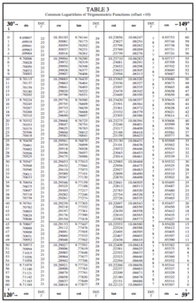
The first published table of logarithms was in John Napier's 1614, Mirifici Logarithmorum Canonis Descriptio. The book contained fifty-seven pages of explanatory matter and ninety pages of tables of trigonometric functions and their natural logarithms.
The English mathematician Henry Briggs visited Napier in 1615, and proposed a re-scaling of Napier's logarithms to form what is now known as the common or base-10 logarithms. Napier delegated to Briggs the computation of a revised table, and they later published, in 1617, Logarithmorum Chilias Prima ("The First Thousand Logarithms"), which gave a brief account of logarithms and a table for the first 1000 integers calculated to the 14th decimal place.
In 1624, Briggs' Arithmetica Logarithmica appeared in folio as a work containing the logarithms of 30,000 natural numbers to fourteen decimal places (1-20,000 and 90,001 to 100,000). This table was later extended by Adriaan Vlacq, but to 10 places, and by Alexander John Thompson to 20 places in 1952.
Briggs was one of the first to use finite-difference methods to compute tables of functions.
Vlacq's table was later found to contain 603 errors, but "this cannot be regarded as a great number, when it is considered that the table was the result of an original calculation, and that more than 2,100,000 printed figures are liable to error." An edition of Vlacq's work, containing many corrections, was issued at Leipzig in 1794 under the title Thesaurus Logarithmorum Completus by Jurij Vega.
François Callet's seven-place table (Paris, 1795), instead of stopping at 100,000, gave the eight-place logarithms of the numbers between 100,000 and 108,000, in order to diminish the errors of interpolation, which were greatest in the early part of the table, and this addition was generally included in seven-place tables. The only important published extension of Vlacq's table was made by Edward Sang in 1871, whose table contained the seven-place logarithms of all numbers below 200,000.
Briggs and Vlacq also published original tables of the logarithms of the trigonometric functions. Briggs completed a table of logarithmic sines and logarithmic tangents for the hundredth part of every degree to fourteen decimal places, with a table of natural sines to fifteen places and the tangents and secants for the same to ten places, all of which were printed at Gouda in 1631 and published in 1633 under the title of Trigonometria Britannica. Tables logarithms of trigonometric functions simplify hand calculations where a function of an angle must be multiplied by another number, as is often the case.
Besides the tables mentioned above, a great collection, called Tables du Cadastre, was constructed under the direction of Gaspard de Prony, by an original computation, under the auspices of the French republican government of the 1790s. This work, which contained the logarithms of all numbers up to 100,000 to nineteen places, and of the numbers between 100,000 and 200,000 to twenty-four places, exists only in manuscript, "in seventeen enormous folios," at the Observatory of Paris. It was begun in 1792, and "the whole of the calculations, which to secure greater accuracy were performed in duplicate, and the two manuscripts subsequently collated with care, were completed in the short space of two years." Cubic interpolation could be used to find the logarithm of any number to a similar accuracy.
For different needs, logarithm tables ranging from small handbooks to multi-volume editions have been compiled:
| Year | Author | Range | Decimal places | Note |
|---|---|---|---|---|
| 1614 | John Napier, Mirifici Logarithmorum Canonis Descriptio | 0°–90°, by minutes | 7 | sin(Θ) & ln(sin(Θ)), see image |
| 1617 | Henry Briggs, Logarithmorum Chilias Prima | 1–1000 | 14 | see image |
| 1624 | Henry Briggs Arithmetica Logarithmica | 1–20,000, 90,000–100,000 | 14 |
|
| 1628 | Adriaan Vlacq | 20,000–90,000 | 10 | contained only 603 errors |
| 1792–94 | Gaspard de Prony Tables du Cadastre | 1–100,000 and 100,000–200,000 | 19 and 24, respectively | "seventeen enormous folios", never published |
| 1794 | Jurij Vega Thesaurus Logarithmorum Completus (Leipzig) | corrected edition of Vlacq's work | ||
| 1795 | François Callet (Paris) | 100,000–108,000 | 7 |
|
| 1871 | Edward Sang | 1–200,000 | 7 |
|
Slide rule


The slide rule was invented around 1620–1630, shortly after John Napier's publication of the concept of the logarithm. Edmund Gunter of Oxford developed a calculating device with a single logarithmic scale; with additional measuring tools it could be used to multiply and divide. The first description of this scale was published in Paris in 1624 by Edmund Wingate (c.1593–1656), an English mathematician, in a book entitled L'usage de la reigle de proportion en l'arithmetique & geometrie. The book contains a double scale, logarithmic on one side, tabular on the other. In 1630, William Oughtred of Cambridge invented a circular slide rule, and in 1632 combined two handheld Gunter rules to make a device that is recognizably the modern slide rule. Like his contemporary at Cambridge, Isaac Newton, Oughtred taught his ideas privately to his students. Also like Newton, he became involved in a vitriolic controversy over priority, with his one-time student Richard Delamain and the prior claims of Wingate. Oughtred's ideas were only made public in publications of his student William Forster in 1632 and 1653.
In 1677, Henry Coggeshall created a two-foot folding rule for timber measure, called the Coggeshall slide rule, expanding the slide rule's use beyond mathematical inquiry.
In 1722, Warner introduced the two- and three-decade scales, and in 1755 Everard included an inverted scale; a slide rule containing all of these scales is usually known as a "polyphase" rule.
In 1815, Peter Mark Roget invented the log log slide rule, which included a scale displaying the logarithm of the logarithm. This allowed the user to directly perform calculations involving roots and exponents. This was especially useful for fractional powers.
In 1821, Nathaniel Bowditch, described in the American Practical Navigator a "sliding rule" that contained scales trigonometric functions on the fixed part and a line of log-sines and log-tans on the slider used to solve navigation problems.
In 1845, Paul Cameron of Glasgow introduced a Nautical Slide-Rule capable of answering navigation questions, including right ascension and declination of the sun and principal stars.
Modern form

A more modern form of slide rule was created in 1859 by French artillery lieutenant Amédée Mannheim, "who was fortunate in having his rule made by a firm of national reputation and in having it adopted by the French Artillery." It was around this time that engineering became a recognized profession, resulting in widespread slide rule use in Europe–but not in the United States. There Edwin Thacher's cylindrical rule took hold after 1881. The duplex rule was invented by William Cox in 1891, and was produced by Keuffel and Esser Co. of New York.
Impact
Writing in 1914 on the 300th anniversary of Napier's tables, E. W. Hobson described logarithms as "providing a great labour-saving instrument for the use of all those who have occasion to carry out extensive numerical calculations" and comparing it in importance to the "Indian invention" of our decimal number system. Napier's improved method of calculation was soon adopted in Britain and Europe. Kepler dedicated his 1620 Ephereris to Napier, congratulating him on his invention and its benefits to astronomy. Edward Wright, an authority on celestial navigation, translated Napier's Latin Descriptio into English in 1615, shortly after its publication. Briggs extended the concept to the more convenient base 10, or common logarithm.
“Probably no work has ever influenced science as a whole, and mathematics in particular, so profoundly as this modest little book [the Descriptio]. It opened the way for the abolition, once and for all, of the infinitely laborious, nay, nightmarish, processes of long division and multiplication, of finding the power and the root of numbers.”
The logarithm function remains a staple of mathematical analysis, but printed tables of logarithms gradually diminished in importance in the twentieth century as mechanical calculators and, later, electronic computers took over computations that required high accuracy. The introduction of hand-held scientific calculators in the 1970s ended the era of slide rules. Logarithmic scale graphs are widely used to display data with a wide range. The decibel, a logarithmic unit, is also widely used. The current, 2002, edition of The American Practical Navigator (Bowditch) still contains tables of logarithms and logarithms of trigonometric functions.
.svg)


![{\displaystyle \ln(z)=\lim _{n\to \infty }n\cdot ({\sqrt[{n}]{z}}-1)}](https://wikimedia.org/api/rest_v1/media/math/render/svg/bba681ea4108b1376919349999b5c3ae9bd08e3b)


![{\displaystyle {\begin{aligned}\ln ab=\int _{1}^{ab}{\frac {1}{x}}\,dx&=\int _{1}^{a}{\frac {1}{x}}\,dx+\int _{a}^{ab}{\frac {1}{x}}\,dx\\[5pt]&=\int _{1}^{a}{\frac {1}{x}}\,dx+\int _{1}^{b}{\frac {1}{at}}a\,dt\\[5pt]&=\int _{1}^{a}{\frac {1}{x}}\,dx+\int _{1}^{b}{\frac {1}{t}}\,dt\\[5pt]&=\ln a+\ln b.\end{aligned}}}](https://wikimedia.org/api/rest_v1/media/math/render/svg/d7210259ed243c3b86451e39eb2b50dccc7832e1)


![{\displaystyle {\begin{aligned}{\frac {d}{dx}}\ln x&=\lim _{h\to 0}{\frac {\ln(x+h)-\ln x}{h}}\\&=\lim _{h\to 0}\left[{\frac {1}{h}}\ln \left({\frac {x+h}{x}}\right)\right]\\&=\lim _{h\to 0}\left[\ln \left(\left(1+{\frac {h}{x}}\right)^{\frac {1}{h}}\right)\right]\quad &&{\text{all above for logarithmic properties}}\\&=\ln \left[\lim _{h\to 0}\left(1+{\frac {h}{x}}\right)^{\frac {1}{h}}\right]\quad &&{\text{for continuity of the logarithm}}\\&=\ln e^{1/x}\quad &&{\text{for the definition of }}e^{x}=\lim _{h\to 0}(1+hx)^{1/h}\\&={\frac {1}{x}}\quad &&{\text{for the definition of the ln as inverse function.}}\end{aligned}}}](https://wikimedia.org/api/rest_v1/media/math/render/svg/7ac40a28d99ea3c3c0e2fbcfad73461fa5837fa6)


![{\displaystyle \ln(x)=(x-1)\prod _{k=1}^{\infty }\left({\frac {2}{1+{\sqrt[{2^{k}}]{x}}}}\right)}](https://wikimedia.org/api/rest_v1/media/math/render/svg/19a685fc50f560fbfd45cd8c625c839137a0cb42)
![{\displaystyle \ln(2)=\left({\frac {2}{1+{\sqrt {2}}}}\right)\left({\frac {2}{1+{\sqrt[{4}]{2}}}}\right)\left({\frac {2}{1+{\sqrt[{8}]{2}}}}\right)\left({\frac {2}{1+{\sqrt[{16}]{2}}}}\right)...}](https://wikimedia.org/api/rest_v1/media/math/render/svg/b7b509b3f7ce72ef554df0dfb48f10dbdc772055)
![{\displaystyle \pi =(2i+2)\left({\frac {2}{1+{\sqrt {i}}}}\right)\left({\frac {2}{1+{\sqrt[{4}]{i}}}}\right)\left({\frac {2}{1+{\sqrt[{8}]{i}}}}\right)\left({\frac {2}{1+{\sqrt[{16}]{i}}}}\right)...}](https://wikimedia.org/api/rest_v1/media/math/render/svg/438561a80d9075271b2dcd15bea94412d2683e69)

![{\displaystyle {\frac {1}{\ln(2)}}=2-{\frac {\sqrt {2}}{2+2{\sqrt {2}}}}-{\frac {\sqrt[{4}]{2}}{4+4{\sqrt[{4}]{2}}}}-{\frac {\sqrt[{8}]{2}}{8+8{\sqrt[{8}]{2}}}}\cdots }](https://wikimedia.org/api/rest_v1/media/math/render/svg/def29e93c87165f8547949c7e10896c45dc22d2f)


![{\displaystyle {\begin{aligned}\ln(1+x)&={\frac {x^{1}}{1}}-{\frac {x^{2}}{2}}+{\frac {x^{3}}{3}}-{\frac {x^{4}}{4}}+{\frac {x^{5}}{5}}-\cdots \\[5pt]&={\cfrac {x}{1-0x+{\cfrac {1^{2}x}{2-1x+{\cfrac {2^{2}x}{3-2x+{\cfrac {3^{2}x}{4-3x+{\cfrac {4^{2}x}{5-4x+\ddots }}}}}}}}}}\end{aligned}}}](https://wikimedia.org/api/rest_v1/media/math/render/svg/92f9f9bda019d60b5ac5d5fd29ea2dd952c5b90a)
![{\displaystyle {\begin{aligned}\ln \left(1+{\frac {x}{y}}\right)&={\cfrac {x}{y+{\cfrac {1x}{2+{\cfrac {1x}{3y+{\cfrac {2x}{2+{\cfrac {2x}{5y+{\cfrac {3x}{2+\ddots }}}}}}}}}}}}\\[5pt]&={\cfrac {2x}{2y+x-{\cfrac {(1x)^{2}}{3(2y+x)-{\cfrac {(2x)^{2}}{5(2y+x)-{\cfrac {(3x)^{2}}{7(2y+x)-\ddots }}}}}}}}\end{aligned}}}](https://wikimedia.org/api/rest_v1/media/math/render/svg/90abfa2132828fc8eea5d3551dfa4df25dbdfa87)
![{\displaystyle {\begin{aligned}\ln 2&=3\ln \left(1+{\frac {1}{4}}\right)+\ln \left(1+{\frac {3}{125}}\right)\\[8pt]&={\cfrac {6}{9-{\cfrac {1^{2}}{27-{\cfrac {2^{2}}{45-{\cfrac {3^{2}}{63-\ddots }}}}}}}}+{\cfrac {6}{253-{\cfrac {3^{2}}{759-{\cfrac {6^{2}}{1265-{\cfrac {9^{2}}{1771-\ddots }}}}}}}}.\end{aligned}}}](https://wikimedia.org/api/rest_v1/media/math/render/svg/bc10de9595aca079ef56e7b76a2a23af56e453da)
![{\displaystyle {\begin{aligned}\ln 10&=10\ln \left(1+{\frac {1}{4}}\right)+3\ln \left(1+{\frac {3}{125}}\right)\\[10pt]&={\cfrac {20}{9-{\cfrac {1^{2}}{27-{\cfrac {2^{2}}{45-{\cfrac {3^{2}}{63-\ddots }}}}}}}}+{\cfrac {18}{253-{\cfrac {3^{2}}{759-{\cfrac {6^{2}}{1265-{\cfrac {9^{2}}{1771-\ddots }}}}}}}}.\end{aligned}}}](https://wikimedia.org/api/rest_v1/media/math/render/svg/931b5e1a786450547bd77e466677d9a983974886)


