Search This Blog

Friday, May 29, 2015

Paradox of a charge in a gravitational field


From Wikipedia, the free encyclopedia

The special theory of relativity is known for its paradoxes: the twin paradox and the ladder-in-barn paradox, for example. Neither are true paradoxes; they merely expose flaws in our understanding, and point the way toward deeper understanding of nature. The ladder paradox exposes the breakdown of simultaneity, while the twin paradox highlights the distinctions of accelerated frames of reference.

So it is with the paradox of a charged particle at rest in a gravitational field; it is a paradox between the theories of electrodynamics and general relativity.

Recap of Key Points of Gravitation and Electrodynamics

It is a standard result from the Maxwell equations of classical electrodynamics that an accelerated charge radiates. That is, it produces an electric field that falls off as 1/r in addition to its rest-frame 1/r^2 Coulomb field. This radiation electric field has an accompanying magnetic field, and the whole oscillating electromagnetic radiation field propagates independently of the accelerated charge, carrying away momentum and energy. The energy in the radiation is provided by the work that accelerates the charge. We understand a photon to be the quantum of the electromagnetic radiation field, but the radiation field is a classical concept.

The theory of general relativity is built on the principle of the equivalence of gravitation and inertia. This means that it is impossible to distinguish through any local measurement whether one is in a gravitational field or being accelerated. An elevator out in deep space, far from any planet, could mimic a gravitational field to its occupants if it could be accelerated continuously "upward". Whether the acceleration is from motion or from gravity makes no difference in the laws of physics. This can also be understood in terms of the equivalence of so-called gravitational mass and inertial mass. The mass in Newton's law of gravity (gravitational mass) is the same as the mass in Newton's second law of motion (inertial mass). They cancel out when equated, with the result discovered by Galileo that all bodies fall at the same rate in a gravitational field, independent of their mass. This was famously demonstrated on the Moon during the Apollo 15 mission, when a hammer and a feather were dropped at the same time and, of course, struck the surface at the same time.

Closely tied in with this equivalence is the fact that gravity vanishes in free fall. For objects falling in an elevator whose cable is cut, all gravitational forces vanish, and things begin to look like the free-floating absence of forces one sees in videos from the International Space Station. One can find the weightlessness of outer space right here on earth: just jump out of an airplane. It is a lynchpin of general relativity that everything must fall together in free fall. Just as with acceleration versus gravity, no experiment should be able to distinguish the effects of free fall in a gravitational field, and being out in deep space far from any forces.

Statement of the Paradox

Putting together these two basic facts of general relativity and electrodynamics, we seem to encounter a paradox. For if we dropped a neutral particle and a charged particle together in a gravitational field, the charged particle should begin to radiate as it is accelerated under gravity, thereby losing energy, and slowing relative to the neutral particle. Then a free-falling observer could distinguish free fall from true absence of forces, because a charged particle in a free-falling laboratory would begin to be pulled relative to the neutral parts of the laboratory, even though no obvious electric fields were present.

Equivalently, we can think about a charged particle at rest in a laboratory on the surface of the earth. Since we know the earth's gravitational field of 1 g is equivalent to being accelerated constantly upward at 1 g, and we know a charged particle accelerated upward at 1 g would radiate, why don't we see radiation from charged particles at rest in the laboratory? It would seem that we could distinguish between a gravitational field and acceleration, because an electric charge apparently only radiates when it is being accelerated through motion, but not through gravitation.

Resolution of the Paradox

The resolution of this paradox, like the twin paradox and ladder paradox, comes through appropriate care in distinguishing frames of reference. We follow the excellent development of Rohrlich (1965),[1] section 8-3, who shows that a charged particle and a neutral particle fall equally fast in a gravitational field, despite the fact that the charged one loses energy by radiation. Likewise, a charged particle at rest in a gravitational field does not radiate in its rest frame. The equivalence principle is preserved for charged particles.

The key is to realize that the laws of electrodynamics, the Maxwell equations, hold only in an inertial frame. That is, in a frame in which no forces act locally. This could be free fall under gravity, or far in space away from any forces. The surface of the earth is not an inertial frame. It is being constantly accelerated. We know the surface of the earth is not an inertial frame because an object at rest there may not remain at rest—objects at rest fall to the ground when released. So we cannot naively formulate expectations based on the Maxwell equations in this frame. It is remarkable that we now understand the special-relativistic Maxwell equations do not hold, strictly speaking, on the surface of the earth—even though they were of course discovered in electrical and magnetic experiments conducted in laboratories on the surface of the earth. Nevertheless, in this case we cannot apply the Maxwell equations to the description of a falling charge relative to a "supported", non-inertial observer.

The Maxwell equations can be applied relative to an observer in free fall, because free-fall is an inertial frame. So the starting point of considerations is to work in the free-fall frame in a gravitational field—a "falling" observer. In the free-fall frame the Maxwell equations have their usual, flat spacetime form for the falling observer. In this frame, the electric and magnetic fields of the charge are simple: the falling electric field is just the Coulomb field of a charge at rest, and the magnetic field is zero. As an aside, note that we are building in the equivalence principle from the start, including the assumption that a charged particle falls equally as fast as a neutral particle. Let us see if any contradictions arise.

Now we are in a position to establish what an observer at rest in a gravitational field, the supported observer, will see. Given the electric and magnetic fields in the falling frame, we merely have to transform those fields into the frame of the supported observer. This is not a Lorentz transformation, because the two frames have a relative acceleration. Instead we must bring to bear the machinery of general relativity.

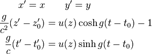
In this case our gravitational field is fictitious because it can be transformed away in an accelerating frame. Unlike the total gravitational field of the earth, here we are assuming that spacetime is locally flat, so that the curvature tensor vanishes. Equivalently, the lines of gravitational acceleration are everywhere parallel, with no convergences measurable in the laboratory. Then the most general static, flat-space, cylindrical metric and line element can be written:

c^2 d\tau^2 = u^2(z)c^2dt^2 - \left ( {c^2\over g} {du\over dz}  \right )^2 dz^2 - dx^2 - dy^2
where c is the speed of light, \tau is proper time, x,y,z,t are the usual coordinates of space and time, g is the acceleration of the gravitational field, and u(z) is an arbitrary function of the coordinate but must approach the observed Newtonian value of 1+gz/c^2. This is the metric for the gravitational field measured by the supported observer.

Meanwhile, the metric in the frame of the falling observer is simply the Minkowski metric:

c^2 d\tau^2 = c^2 dt'^2 - dz'^2 - dy'^2 -dz'^2
From these two metrics Rohrlich constructs the coordinate transformation between them:
\begin{align}
x'=x &\qquad y'=y  \\
{g\over c^2} (z'-z_0') &= u(z) \cosh{g(t-t_0)} -1\\
{g\over c} (t'-t_0') &= u(z) \sinh{g(t-t_0) }
\end{align}
When this coordinate transformation is applied to the rest frame electric and magnetic fields of the charge, it is found to be radiating—as expected for a charge falling away from a supported observer. Rohrlich emphasizes that this charge remains at rest in its free-fall frame, just as a neutral particle would. Furthermore, the radiation rate for this situation is Lorentz invariant, but it is not invariant under the coordinate transformation above, because it is not a Lorentz transformation.

So a falling charge will appear to radiate to a supported observer, as expected. What about a supported charge, then? Does it not radiate due to the equivalence principle? To answer this question, start again in the falling frame.
In the falling frame, the supported charge appears to be accelerated uniformly upward. The case of constant acceleration of a charge is treated by Rohrlich [1] in section 5-3. He finds a charge e uniformly accelerated at rate g has a radiation rate given by the Lorentz invariant:

R={2\over 3}{e^2\over c^3} g^2
The corresponding electric and magnetic fields of an accelerated charge are also given in Rohrlich section 5-3. To find the fields of the charge in the supported frame, the fields of the uniformly accelerated charge are transformed according to the coordinate transformation previously given. When that is done, one finds no radiation in the supported frame from a supported charge, because the magnetic field is zero in this frame. Rohrlich does note that the gravitational field slightly distorts the Coulomb field of the supported charge, but too small to be observable. So although the Coulomb law was of course discovered in a supported frame, relativity tells us the field of such a charge is not precisely 1/r^2.

The radiation from the supported charge is something of a curiosity: where does it go? Boulware (1980) [2] finds that the radiation goes into a region of spacetime inaccessible to the co-accelerating, supported observer. In effect, a uniformly accelerated observer has an event horizon, and there are regions of spacetime inaccessible to this observer. de Almeida and Saa (2006) [3] have a more-accessible treatment of the event horizon of the accelerated observer.

Global climate on verge of multi-decadal change

Date:  May 27, 2015
 
Source:  University of Southampton
 
Original link:  http://www.sciencedaily.com/releases/2015/05/150527133932.htm
 
Summary
 
The global climate is on the verge of broad-scale change that could last for a number of decades a new study implies. The change to the new set of climatic conditions is associated with a cooling of the Atlantic, and is likely to bring drier summers in Britain and Ireland, accelerated sea-level rise along the northeast coast of the United States, and drought in the developing countries of the Sahel region.
The RAPID moorings being deployed.
Credit: National Oceanography Centre

A new study, by scientists from the University of Southampton and National Oceanography Centre (NOC), implies that the global climate is on the verge of broad-scale change that could last for a number of decades.

The change to the new set of climatic conditions is associated with a cooling of the Atlantic, and is likely to bring drier summers in Britain and Ireland, accelerated sea-level rise along the northeast coast of the United States, and drought in the developing countries of the Sahel region. Since this new climatic phase could be half a degree cooler, it may well offer a brief reprise from the rise of global temperatures, as well as resulting in fewer hurricanes hitting the United States.

The study, published in Nature, proves that ocean circulation is the link between weather and decadal scale climatic change. It is based on observational evidence of the link between ocean circulation and the decadal variability of sea surface temperatures in the Atlantic Ocean.

Lead author Dr Gerard McCarthy, from the NOC, said: "Sea-surface temperatures in the Atlantic vary between warm and cold over time-scales of many decades. These variations have been shown to influence temperature, rainfall, drought and even the frequency of hurricanes in many regions of the world. This decadal variability, called the Atlantic Multi-decadal Oscillation (AMO), is a notable feature of the Atlantic Ocean and the climate of the regions it influences."

These climatic phases, referred to as positive or negative AMO's, are the result of the movement of heat northwards by a system of ocean currents. This movement of heat changes the temperature of the sea surface, which has a profound impact on climate on timescales of 20-30 years. The strength of these currents is determined by the same atmospheric conditions that control the position of the jet stream. Negative AMO's occur when the currents are weaker and so less heat is carried northwards towards Europe from the tropics.

The strength of ocean currents has been measured by a network of sensors, called the RAPID array, which have been collecting data on the flow rate of the Atlantic meridonal overturning circulation (AMOC) for a decade.

Dr David Smeed, from the NOC and lead scientist of the RAPID project, adds: "The observations of AMOC from the RAPID array, over the past ten years, show that it is declining. As a result, we expect the AMO is moving to a negative phase, which will result in cooler surface waters. This is consistent with observations of temperature in the North Atlantic."

Since the RAPID array has only been collecting data for last ten years, a longer data set was needed to prove the link between ocean circulation and slow climate variations. Therefore this study instead used 100 years of sea level data, maintained by the National Oceanography Centre's permanent service for mean sea level. Models of ocean currents based on this data were used to predict how much heat would be transported around the ocean, and the impact this would have on the sea surface temperature in key locations.

Co-author Dr Ivan Haigh, lecturer in coastal oceanography at the University of Southampton, said: "By reconstructing ocean circulation over the last 100 years from tide gauges that measure sea level at the coast, we have been able to show, for the first time, observational evidence of the link between ocean circulation and the AMO."

Story Source:

The above story is based on materials provided by University of Southampton. Note: Materials may be edited for content and length.

Journal Reference:
  1. Gerard D. McCarthy, Ivan D. Haigh, Joël J.-M. Hirschi, Jeremy P. Grist, David A. Smeed. Ocean impact on decadal Atlantic climate variability revealed by sea-level observations. Nature, 2015; 521 (7553): 508 DOI: 10.1038/nature14491

Retracted Scientific Studies: A Growing List

Haruko Obokata, the lead scientist of a retracted stem cell study, at a news conference last year. Credit Kimimasa Mayama/European Pressphoto Agency
The retraction by Science of a study of changing attitudes about gay marriage is the latest prominent withdrawal of research results from scientific literature. And it very likely won't be the last. A 2011 study in Nature found a 10-fold increase in retraction notices during the preceding decade.

Many retractions barely register outside of the scientific field. But in some instances, the studies that were clawed back made major waves in societal discussions of the issues they dealt with. This list recounts some prominent retractions that have occurred since 1980.
  1. Vaccines and Autism

    In 1998, The Lancet, a British medical journal, published a study by Dr. Andrew Wakefield that suggested that autism in children was caused by the combined vaccine for measles, mumps and rubella. In 2010, The Lancet retracted the study following a review of Dr. Wakefield's scientific methods and financial conflicts.
    Despite challenges to the study, Dr. Wakefield's research had a strong effect on many parents. Vaccination rates tumbled in Britain, and measles cases grew. American antivaccine groups also seized on the research. The United States had more cases of measles in the first month of 2015
    than the number that is typically diagnosed in a full year.

  2.  Stem Cell Production

    Papers published by Japanese researchers in Nature in 2014 claimed to provide an easy method to create multipurpose stem cells, with eventual implications for the treatment of diseases and injuries. Months later, the authors, including Haruko Obokata, issued a retraction. An investigation by one of Japan's most prestigious scientific institutes, where much of the research occurred, found that the author had manipulated some of the images published in the study.

    Approximately one month after the retraction, one of Ms. Obokata's co-authors, Yoshiki Sasai, was found hanging in a stairwell of his office. He had taken his own life.
  3. Photo
    Cloning and Human Stem Cells

    Papers in 2004 and 2005 in the journal Science pointed to major progress in human cloning and the extraction of stem cells. When it became clear that much of the data was fabricated, Science eventually retracted both papers.

    Hwang Woo Suk, the lead author of the papers, was later convicted of embezzlement and bioethical violations in South Korea. In the years since his conviction, Dr. Hwang has continued working in the field, and was awarded an American patent in 2014 for the fraudulent work.

  4. John Darsee's Heart Research

    In 1983, Dr. John Darsee, a heart researcher at both Harvard Medical School and Emory University, was caught faking data in most of his 100 published pieces. That Dr. Darsee managed to slip through the system undetected for 14 years revealed, said Dr. Eugene Braunwald, his former superior at Harvard, ''the extraordinary difficulty of detecting fabrication by a clever individual.'' Dr. Darsee was barred from receiving federal funds for 10 years.

  5. Physics Discoveries at Bell Labs

    Between 1998 and 2001, Bell Labs announced a series of major breakthroughs in physics, including the creation of molecular-scale transistors. A panel found that 17 papers relied on fraudulent data, and blamed one scientist, J. Hendrik Schön. It did not fault Mr. Schön's co-authors. In 2004, the University of Konstanz in Germany stripped Mr. Schön of his Ph.D.

  6. Cancer in Rats and Herbicides

    The journal Food and Chemical Toxicology published a paper in 2012 that seemed to show that genetically modified corn and the herbicide Roundup caused premature death in rats resulting from cancer. In 2013, the journal retracted the study, finding that the number of rats studied had been too small, and that the strain of rats had prone to cancer. The lead author, Gilles-Eric Séralini, was not accused of fraud, and the paper was republished in 2014 in another journal.

  7. Pesticides and Estrogen

    A 1996 report in Science said mixtures of some pesticides might be endocrine disruptors and lead to a rise in estrogen hormones, causing cancer and birth defects in humans and animals. In 1997, the paper was withdrawn after its senior author, John A. McLachlan, admitted the results could not be reproduced. The paper's publication affected federal legislation and set off a frantic round of research.

  8. Diederik Stapel's Psychology Research 
     
    Several dozen published papers by Diederik Stapel, a psychology researcher at Tilburg University in the Netherlands, were based on falsified data and faked experiments. Dr. Stapel's studies, like one that found eating meat made people selfish, generated considerable media attention. Dr. Stapel admitted in an interview that his frauds were driven by "a quest for aesthetics, for beauty — instead of the truth."

  9. Marc Hauser's Cognition Research

    In 2010, Harvard University found that Marc Hauser, a researcher in animal and human cognition, had committed eight instances of scientific misconduct. Dr. Hauser retracted a 2002 paper in the journal Cognition about rule learning in monkeys, and corrected his research in other papers. A federal investigation also found that Dr. Hauser had committed fraud. Dr. Hauser left his post at Harvard in 2011.

Anti-GMO stance by Greenpeace, other environmental activists, worsen climate change

| May 28, 2015 |
 
Original link:  http://www.geneticliteracyproject.org/2015/05/28/anti-gmo-stance-by-greenpeace-other-environmental-activists-worsens-climate-change/ 
 
Unknown

Pretend for a moment that you lead an environmental group, dedicated to eliminating the causes of global climate change. As such an environmental leader, you’d be excited about a technology change that reduces the greenhouse gases behind climate change, right? Especially if this technology already has reduced greenhouse gas by the equivalent of nearly 12 million automobiles?

Not if that technology is genetically modified food. Non-government organizations that have taken a strident anti-GMO stance, like Greenpeace, resist any connection between climate change and genetically modified agriculture. Biotechnology isn’t even a significant concept in climate change efforts, particularly in Europe. Worse, this resistance isn’t as scientific as it is political.

A recent study by Philipp Aerni at the University of Zurich evaluated 55 representatives of 44 organizations that included business, US, European and Asian government agencies, academic institutions, organizations like the Intergovernmental Panel on Climate Change (IPCC), The World Bank/International Monetary Fund, Greenpeace, the World Wildlife Fund, and the Bill and Melinda Gates Foundation. Most of the participants looked favorably upon biotechnology and genetic modifications of crops, with the exception of a small number of advocacy groups, the most well-known of which was Greenpeace. But while participants were more willing to privately favor biotechnology as a source of solutions to climate change, few were willing to express that sentiment publicly. Aerni wrote:
Since core stakeholders in both debates (Greenpeace and the World Wildlife Fund are involved with both climate change and GMO issues) radically oppose the use of modern biotechnology, and can count on widespread public support, especially in affluent countries,…other stakeholders may also side with the popular view, even if that view may not be in line with their more pragmatic personal view.
Biotechnology may not be ‘clean tech’ as long as powerful environmental groups say it is not.
Science versus “because I said so”

Greenpeace, for its part, repeatedly points to three areas to show that “GM crops fail in climate change conditions:”
  • It cites a 2005 study that allegedly shows that “temperature fluctuations caused crop losses in GM cotton in China.” However the study only shows a drop in Bt Cry protein production in very hot conditions; no mention is made of crop loss. In fact, other studies show similar effects of heat on any kind of cotton, regardless of breeding.
  • The organization claims that GM soybeans “suffered unexpected losses in the US during hot weather,” citing a news report on a study conducted in 1999. However, scientists who read the study discovered that it did not even mention yield loss. Instead, they read about a loss of total crop that was marginally worse than conventional grown soybeans.
  • Finally, it blames monoculture and loss of biodiversity on genetically modified crops, which we have seen have nothing directly to do with genetic modifications of plants. Monoculture is an over-simplistic designation, and is an issue with any kind of large-scale agriculture.
The GM Contribution

Genetic modification has made significant inroads into curbing climate change. Drought- and salt-tolerant GM plants have been produced, and researchers are looking into developing more. Thriving under extreme heat also is an area of keen interest.

As for helping to prevent climate change in the first place, GM has not been much of a slouch. Adopting GM technology has reduced pesticide spraying by nearly 9 percent. This arises from replacing broad-range pesticides with glyphosate and in some cases 2,4D, reducing the volume of pesticides used and the fossil fuel needed to spray them.

In addition, tillage, necessary for organic and some conventional farming, is usually not necessary for genetically modified crops. A Purdue University study found that no-till fields released 57 percent less nitrous oxide (another greenhouse gas) than fields that required tillage. Thus, less tillage sequesters more carbon and nitrogen in soil.

Finally, genetic modifications produce crops that can get higher yields using less space. This means that less land needs to be disrupted—fewer trees are removed, more plants are preserved and less carbon is released (not to mention the carbon dioxide taken up by plants). The USDA recently found that organic agriculture would require almost twice and much land than is necessary using conventional methods (measured against GM crops, that number’s more dramatic. Organic agriculture would require an extra 121.7 million acres to grow all US-produced food—that’s an area the size of Spain.

Together, reducing spraying and tillage saved 2.1 billion kilograms of carbon dioxide in 2012 alone. This means tons of carbon that isn’t released into the atmosphere, carbon that isn’t burned by crop dusters and other sprayers, and reduction in land use needed for agricultural production.

As for Greenpeace and other anti-GMO groups, organic remains a more viable alternative than GM, even in the face of organic’s threats to climate change.

Ramez Naam, author of The Infinite Resource: The Power of Ideas on a Finite Planet, recently wrote in the Genetic Literacy Project that “Organic farming is environmentally kinder to every acre of land. But it requires more acres.  The trade-off is a harsh one. Would we rather have pesticides on farmland and nitrogen runoffs from them? Or would we rather chop down more forest? How much more forest would we have to chop down?”

What we’re facing

As the world population increases, it’s estimated that demand for food will increase 70 percent over the next 40 years. This means we need higher yields, and more efficient ways of maintaining a secure, safe food supply. At the same time, efforts to reduce (or even reverse) climate change call for conservation of green plants and activities that do not release more greenhouse gases into the atmosphere. To the participants in Aerni’s Swiss study, they knew that the plant can’t leave any technology unturned. Unfortunately, louder public voices are shouting them down.

Andrew Porterfield is a writer, editor and communications consultant for academic institutions, companies and non-profits in the life sciences. He is based in Camarillo, California. Follow @AMPorterfield on Twitter.

New paper finds a large warming bias in Northern Hemisphere temperatures from 'non-valid' station data

Original linkhttp://hockeyschtick.blogspot.ca/2015/05/new-paper-finds-large-warming-bias-in.html
 
A new paper published in the Journal of Atmospheric and Solar-Terrestrial Physics finds that the quality of Northern Hemisphere temperature data has significantly & monotonically decreased since the year 1969, and that the continued use of 'non-valid' weather stations in calculating Northern Hemisphere average temperatures has created a 'positive bias' and "overestimation of temperatures after including non-valid stations." 

The paper appears to affirm a number of criticisms of skeptics that station losses, fabricated/infilled data, and positively-biased 'adjustments' to temperature data have created a positive skew to the data and overestimation of warming during the 20th and 21st centuries. 

Graphs from the paper below show that use of both valid and 'non-valid' station data results in a mean annual Northern Hemisphere temperature over 1C warmer at the end of the record in 2013 as compared to use of 'valid' weather station data exclusively. 

In addition, the paper shows that use of the sharply decreasing number of stations with valid data produces a huge spike in Northern Hemisphere temperatures around ~2004, which is in sharp contrast to much more comprehensive satellite data showing a 'pause' or even cooling over the same period, further calling into question the quality of even the 'valid' land-based stations (urban heat island effects perhaps?).

"The number of valid weather stations is monotonically decreasing after 1969" is shown by the dashed line, and has resulted in an "overestimation of temperature after including non-valid stations" shown by the solid line, especially a spike in temperature in the early 21st century that is not found in satellite temperature records. 
Using temperature data from "valid" stations only, and a base period of 1961-1990, the warmest temperatures were in the first half of the 20th century.
Using a base period of 1800-2013 (including 'non-valid' stations) shows a temperature spike beginning in the early 21st century, but this is not found in the much more accurate and spatially comprehensive satellite records. 
"The computed average by using all stations [including invalid stations, dashed line] is always greater than from using only valid [stations, solid line at bottom of chart]. Percentage of valid stations has steadily declined since 1969 [shown in grey shaded area]. 

Highlights

Introduce the concept of a valid station and use for computations.
Define indices for data quality and seasonal bias and use for data evaluation.
Compute averages for mean and five point summary plus standard deviations.
Indicate a monotonically decreasing data quality after the year 1969.
Observe an overestimation of temperature after including non-valid stations.

Abstract

Starting from a set of 6190 meteorological stations we are choosing 6130 of them and only for Northern Hemisphere we are computing average values for absolute annual MeanMinimumQ1, MedianQ3,Maximum temperature plus their standard deviations for years 1800–2013, while we use 4887 stations and 389 467 rows of complete yearly data. The data quality and the seasonal bias indices are defined and used in order to evaluate our dataset. After the year 1969 the data quality is monotonically decreasing while the seasonal bias is positive in most of the cases. An Extreme Value Distribution estimation is performed for minimum and maximum values, giving some upper bounds for both of them and indicating a big magnitude for temperature changes. Finally suggestions for improving the quality of meteorological data are presented

Relativistic electromagnetism


From Wikipedia, the free encyclopedia

This article is about a simplified presentation of electromagnetism, incorporating special relativity. For a more general article on the relationship between special relativity and electromagnetism, see Classical electromagnetism and special relativity. For a more rigorous discussion, see Covariant formulation of classical electromagnetism.
Relativistic electromagnetism is a modern teaching strategy for developing electromagnetic field theory from Coulomb's law and Lorentz transformations. Though Coulomb's law expresses action at a distance, it is an easily understood electric force principle. The more sophisticated view of electromagnetism expressed by electromagnetic fields in spacetime can be approached by applying spacetime symmetries. In certain special configurations it is possible to exhibit magnetic effects due to relative charge density in various simultaneous hyperplanes. This approach to physics education and the education and training of electrical and electronics engineers can be seen in the Encyclopædia Britannica (1956), The Feynman Lectures on Physics (1964), Edward M. Purcell (1965), Jack R. Tessman (1966), W.G.V. Rosser (1968), Anthony French (1968), and Dale R. Corson & Paul Lorrain (1970). This approach provides some preparation for understanding of magnetic forces involved in the Biot–Savart law, Ampère's law, and Maxwell's equations.

In 1912 Leigh Page expressed the aspiration of relativistic electromagnetism:[1]
If the principle of relativity had been enunciated before the date of Oersted’s discovery, the fundamental relations of electrodynamics could have been predicted on theoretical grounds as a direct consequence of the fundamental laws of electrostatics, extended so as to apply to charges relatively in motion as well as charges relatively at rest.

Einstein's motivation

In 1953 Albert Einstein wrote to the Cleveland Physics Society on the occasion of a commemoration of the Michelson–Morley experiment. In that letter he wrote:[2]
What led me more or less directly to the special theory of relativity was the conviction that the electromotive force acting on a body in motion in a magnetic field was nothing else but an electric field.
This statement by Einstein reveals that he investigated spacetime symmetries to determine the complementarity of electric and magnetic forces.

Introduction

Purcell argued that the question of an electric field in one inertial frame of reference, and how it looks from a different reference frame moving with respect to the first, is crucial to understand fields created by moving sources. In the special case, the sources that create the field are at rest with respect to one of the reference frames. Given the electric field in the frame where the sources are at rest, Purcell asked: what is the electric field in some other frame?
He stated that the fundamental assumption is that, knowing the electric field at some point (in space and time) in the rest frame of the sources, and knowing the relative velocity of the two frames provided all the information needed to calculate the electric field at the same point in the other frame. In other words, the electric field in the other frame does not depend on the particular distribution of the source charges, only on the local value of the electric field in the first frame at that point. He assumed that the electric field is a complete representation of the influence of the far-away charges.

Alternatively, introductory treatments of magnetism introduce the Biot–Savart law, which describes the magnetic field associated with an electric current. An observer at rest with respect to a system of static, free charges will see no magnetic field. However, a moving observer looking at the same set of charges does perceive a current, and thus a magnetic field.

Uniform electric field — simple analysis


Figure 1: Two oppositely charged plates produce uniform electric field even when moving. The electric field is shown as 'flowing' from top to bottom plate. The Gaussian pill box (at rest) can be used to find the strength of the field.

Consider the very simple situation of a charged parallel-plate capacitor, whose electric field (in its rest frame) is uniform (neglecting edge effects) between the plates and zero outside.

To calculate the electric field of this charge distribution in a reference frame where it is in motion, suppose that the motion is in a direction parallel to the plates as shown in figure 1. The plates will then be shorter by a factor of:
 \sqrt{1 - v^2/c^2}
than they are in their rest frame, but the distance between them will be the same. Since charge is independent of the frame in which it is measured, the total charge on each plate is also the same. So the charge per unit area on the plates is therefore larger than in the rest frame by a factor of:
 1\over\sqrt{1 - v^2/c^2}
The field between the plates is therefore stronger by this factor.

More rigorous analysis


Figure 2a: The electric field lines are shown flowing outward from the positive plate

Figure 2b: The electric field lines flow inward toward the negative plate

Consider the electric field of a single, infinite plate of positive charge, moving parallel to itself. The field must be uniform both above and below the plate, since it is uniform in its rest frame. We also assume that knowing the field in one frame is sufficient for calculating it in the other frame.

The plate however could have a non zero component of electric field in the direction of motion as in Fig 2a. Even in this case, the field of the infinite plane of negative charge must be equal and opposite to that of the positive plate (as in Fig 2b), since the combination of plates is neutral and cannot therefore produce any net fields. When the plates are separated, the horizontal components still cancel, and the resultant is a uniform vertical field as shown in Fig 1.

If Gauss's law is applied to pillbox as shown in Fig 1, it can be shown that the magnitude of the electric field between the plates is given by:
 |E'|= {\sigma' \over\epsilon_0}\
where the prime (') indicates the value measured in the frame in which the plates are moving.  \sigma represents the surface charge density of the positive plate. Since the plates are contracted in length by the factor
 \sqrt{1 - v^2/c^2}
then the surface charge density in the primed frame is related to the value in the rest frame of the plates by:
\sigma'\ = {\sigma\over\sqrt{1 - v^2/c^2}}
But the electric field in the rest frame has value σ / ε0 and the field points in the same direction on both of the frames, so
E' = {E\over\sqrt{1 - v^2/c^2}}\
The E field in the primed frame is therefore stronger than in the unprimed frame. If the direction of motion is perpendicular to the plates, length contraction of the plates does not occur, but the distance between them is reduced. This closer spacing however does not affect the strength of the electric field. So for motion parallel to the electric field E,
E' = E \
In the general case where motion is in a diagonal direction relative to the field the field is merely a superposition of the perpendicular and parallel fields., each generated by a set of plates at right angles to each other as shown in Fig 3. Since both sets of plates are length contracted, the two components of the E field are
E'_y = {E_y\over\sqrt{1 - v^2/c^2}}
and
 E'_x = E_x \
where the y subscript denotes perpendicular, and the x subscript, parallel.
These transformation equations only apply if the source of the field is at rest in the unprimed frame.

The field of a moving point charge[edit]


Figure 3: A point charge at rest, surrounded by an imaginary sphere.

Figure 4: A view of the electric field of a point charge moving at constant velocity.

A very important application of the electric field transformation equations is to the field of a single point charge moving with constant velocity. In its rest frame, the electric field of a positive point charge has the same strength in all directions and points directly away from the charge. In some other reference frame the field will appear differently.

In applying the transformation equations to a nonuniform electric field, it is important to record not only the value of the field, but also at what point in space it has this value.

In the rest frame of the particle, the point charge can be imagined to be surrounded by a spherical shell which is also at rest. In our reference frame, however, both the particle and its sphere are moving. Length contraction therefore states that the sphere is deformed into an oblate spheroid, as shown in cross section in Fig 4.

Consider the value of the electric field at any point on the surface of the sphere. Let x and y be the components of the displacement (in the rest frame of the charge), from the charge to a point on the sphere, measured parallel and perpendicular to the direction of motion as shown in the figure. Because the field in the rest frame of the charge points directly away from the charge, its components are in the same ratio as the components of the displacement:
{E_y \over E_x} = {y \over x}
In our reference frame, where the charge is moving, the displacement x' in the direction of motion is length-contracted:
x' = x\sqrt{1 - v^2/c^2}
The electric field at any point on the sphere points directly away from the charge. (b) In a reference frame where the charge and the sphere are moving to the right, the sphere is length-contracted but the vertical component of the field is stronger. These two effects combine to make the field again point directly away from the current location of the charge. (While the y component of the displacement is the same in both frames).

However, according to the above results, the y component of the field is enhanced by a similar factor:
E'_y = {E_y\over\sqrt{1 - v^2/c^2}}
whilst the x component of the field is the same in both frames. The ratio of the field components is therefore
{E'_y \over E'_x} = {E_y \over E_x\sqrt{1 - v^2/c^2}} = {y' \over x'}
So, the field in the primed frame points directly away from the charge, just as in the unprimed frame. A view of the electric field of a point charge moving at constant velocity is shown in figure 4. The faster the charge is moving, the more noticeable the enhancement of the perpendicular component of the field becomes. If the speed of the charge is much less than the speed of light, this enhancement is often negligible. But under certain circumstances, it is crucially important even at low velocities.

The origin of magnetic forces


Figure 5, lab frame: A horizontal wire carrying a current, represented by evenly spaced positive charges moving to the right whilst an equal number of negative charges remain at rest, with a positively charged particle outside the wire and traveling in a direction parallel to the current.

In the simple model of events in a wire stretched out horizontally, a current can be represented by the evenly spaced positive charges, moving to the right, whilst an equal number of negative charges remain at rest. If the wire is electrostatically neutral, the distance between adjacent positive charges must be the same as the distance between adjacent negative charges.

Assume that in our 'lab frame' (Figure 5), we have a positive test charge, Q, outside the wire, traveling parallel to the current, at the speed, v, which is equal to the speed of the moving charges in the wire. It should experience a magnetic force, which can be easily confirmed by experiment.

Figure 6, test charge frame: The same situation as in fig. 5, but viewed from the reference frame in which positive charges are at rest. The negative charges flow to the left. The distance between the negative charges is length-contracted relative to the lab frame, while the distance between the positive charges is expanded, so the wire carries a net negative charge.

Inside 'test charge frame'(Fig. 6), the only possible force is the electrostatic force Fe = Q * E because, although the magnetic field is the same, the test charge is at rest and, therefore, cannot feel it. In this frame, the negative charge density has Lorentz-contracted with respect to what we had in lab frame because of the increased speed. This means that spacing between charges has reduced by the Lorentz factor with respect to the lab frame spacing, l:
 l_- = {l\sqrt{1-v^2/c^2}}
Thus, positive charges have Lorentz-expanded (because their speed has dropped):
 l_+ = l / \sqrt{1-v^2/c^2}
Both of these effects combine to give the wire a net negative charge in the test charge frame. Since the negatively charged wire exerts an attractive force on a positively charged particle, the test charge will therefore be attracted and will move toward the wire.

For v << c, we can concretely compute both,[3] the magnetic force sensed in the lab frame
 F_m = {Q v I \over 2 \pi \epsilon _0 c^2 R}
and electrostatic force, sensed in the test charge frame, where we first compute the charge density with respect to the lab frame length, l:
 \lambda = {q \over l}_+ - {q \over l}_- = {q \over l}(\sqrt{1-v^2/c^2} - 1/\sqrt{1-v^2/c^2}) \approx {q \over l}(1-0.5({v^2\over c^2}) - 1 - 0.5({v^2\over c^2})) = -{q \over l}{v^2\over c^2}
and, keeping in mind that current I = {q\over t} = q{v\over l}, resulting electrostatic force
 F_e = Q E = Q  {\lambda \over 2 \pi \epsilon _0 R} = {Q q v^2 \over 2 \pi \epsilon _0 c^2 R l} = {Q v I\over 2 \pi \epsilon _0 c^2 R }
which comes out exactly equal to the magnetic force sensed in the lab frame, F_e = F_m.

The lesson is that observers in different frames of reference see the same phenomena but disagree on their reasons.
If the currents are in opposite directions, consider the charge moving to the left. No charges are now at rest in the reference frame of the test charge. The negative charges are moving with speed v in the test charge frame so their spacing is again:
 l_{(-)} = {l\sqrt{1-v^2/c^2}}
The distance between positive charges is more difficult to calculate. The relative velocity should be less than 2v due to special relativity. For simplicity, assume it is 2v. The positive charge spacing contraction is then:
 {\sqrt{1-(2v/c)^2}}
relative to its value in their rest frame. Now its value in their rest frame was found to be
 l_{(+)} = {l\over\sqrt{1-v^2/c^2}}
So the final spacing of positive charges is:
 l_{(+)} = {l\over\sqrt{1-v^2/c^2}}{\sqrt{1-(2v/c)^2}}
To determine whether l(+) or l(-) is larger we assume that v << c and use the binomial approximation that
(1+x)^p \approxeq 1+px\mbox{ when }x<<1
After some algebraic calculation it is found that l(+) < l(-), and so the wire is positively charged in the frame of the test charge.[4]

One may think that the picture, presented here, is artificial because electrons, which accelerated in fact, must condense in the lab frame, making the wire charged. Naturally, however, all electrons feel the same accelerating force and, therefore, identically to the Bell's spaceships, the distance between them does not change in the lab frame (i.e. expands in their proper moving frame). Rigid bodies, like trains, don't expand however in their proper frame, and, therefore, really contract, when observed from the stationary frame.

Calculating the magnetic field

The Lorentz force law

A moving test charge near a wire carrying current will experience a magnetic force dependent on the velocity of the moving charges in the wire. If the current is flowing to the right, and a positive test charge is moving below the wire, then there is a force in a direction 90° counterclockwise from the direction of motion.

The magnetic field of a wire

Calculation of the magnitude of the force exerted by a current-carrying wire on a moving charge is equivalent to calculating the magnetic field produced by the wire. Consider again the situation shown in figures. The latter figure, showing the situation in the reference frame of the test charge, is reproduced in the figure. The positive charges in the wire, each with charge q, are at rest in this frame, while the negative charges, each with charge −q, are moving to the left with speed v. The average distance between the negative charges in this frame is length-contracted to:
 \sqrt{1 - v^2/c^2}
where is the distance between them in the lab frame. Similarly, the distance between the positive charges is not length-contracted:
 \sqrt{1 - v^2/c^2}
Both of these effects give the wire a net negative charge in the test charge frame, so that it exerts an attractive force on the test charge.

1947–1948 civil war in Mandatory Palestine

From Wikipedia, the free encyclopedia During the civil war, the Jewish and Arab communities of Palestine clashed (the latter supported b...