
Southern Oscillation Index timeseries 1876–2012.
El Niño Southern Oscillation (
ENSO) is an irregularly periodical climate change caused by variations in
sea surface temperatures over the tropical eastern Pacific Ocean, affecting much of the tropics and subtropics. The warming phase is known as
El Niño and the cooling phase as
La Niña. The two variations are coupled:
El Niño is accompanied with high, and
La Niña with low air
surface pressure in the tropical western Pacific.
[1][2] The two periods last several years each (typically three to four) and their effects vary in intensity.
[3]
The two phases relate to the
Walker circulation, discovered by
Gilbert Walker during the early twentieth century. The Walker circulation is caused by the
pressure gradient force that results from a
high pressure system over the eastern Pacific ocean, and a
low pressure system over
Indonesia. When the Walker circulation weakens or reverses, an
El Niño results, causing the ocean surface to be warmer than average, as upwelling of cold water occurs less or not at all. An especially strong Walker circulation causes a
La Niña, resulting in cooler ocean temperatures due to increased upwelling.
Mechanisms that cause the oscillation remain under study. The extremes of this climate pattern's oscillations cause extreme weather (such as floods and droughts) in many regions of the world. Developing countries dependent upon agriculture and fishing, particularly those bordering the Pacific Ocean, are the most affected.
Gilbert Walker
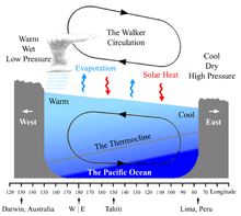
Diagram of the quasi-equilibrium and
La Niña phase of the Southern Oscillation. The Walker circulation is seen at the surface as easterly trade winds which move water and air warmed by the sun towards the west. The western side of the equatorial Pacific is characterized by warm, wet low pressure weather as the collected moisture is dumped in the form of typhoons and thunderstorms. The ocean is some 60 centimetres (24 in) higher in the western Pacific as the result of this motion. The water and air are returned to the east. Both are now much cooler, and the air is much drier. An El Niño episode is characterised by a breakdown of this water and air cycle, resulting in relatively warm water and moist air in the eastern Pacific.
Gilbert Walker was an established applied mathematician at the
University of Cambridge when he became director-general of observatories in India in 1904.
[4] While there, he studied the characteristics of the
Indian Ocean monsoon, the failure of whose rains had brought severe
famine to the country in 1899. Analyzing vast amounts of weather data from India and lands beyond, over the next fifteen years he published the first descriptions of the great seesaw oscillation of
atmospheric pressure between the Indian and
Pacific Ocean, and its correlation to
temperature and
rainfall patterns across much of the Earth's tropical regions, including India. He also worked with the
Indian Meteorological Department especially in linking the
monsoon with Southern Oscillation phenomenon. He was made a Companion of the
Order of the Star of India in 1911.
[4]
Southern Oscillation

Normal Pacific pattern: Equatorial winds gather warm water pool toward the west. Cold water upwells along South American coast. (
NOAA /
PMEL / TAO)
The Southern Oscillation is the atmospheric component of El Niño. This component is an oscillation in surface air pressure between the tropical eastern and the western
Pacific Ocean waters. The strength of the Southern Oscillation is measured by the
Southern Oscillation Index (
SOI). The SOI is computed from fluctuations in the surface air pressure difference between
Tahiti (in the Pacific) and
Darwin, Australia (on the Indian Ocean).
[5]
- El Niño episodes have negative SOI, meaning there is lower pressure over Tahiti and higher pressure in Darwin.
- La Niña episodes have positive SOI, meaning there is higher pressure in Tahiti and lower in Darwin.
Low atmospheric pressure tends to occur over warm water and high pressure occurs over cold water, in part because of deep convection over the warm water. El Niño episodes are defined as sustained warming of the central and eastern tropical Pacific Ocean, thus resulting in a decrease in the strength of the Pacific
trade winds, and a reduction in rainfall over eastern and northern Australia. La Niña episodes are defined as sustained cooling of the central and eastern tropical Pacific Ocean, thus resulting in an increase in the strength of the Pacific
trade winds, and the opposite effects in Australia when compared to El Niño.
El Niño conditions: Warm water pool approaches the South American coast. The absence of cold upwelling increases warming.

La Niña conditions: Warm water is farther west than usual.
Although the Southern Oscillation Index has a long station record going back to the 1800s, its reliability is limited due to the presence of both Darwin and Tahiti well south of the Equator, resulting in the surface air pressure at both locations being less directly related to ENSO.
[6] To overcome this question, a new index was created, being named
Equatorial Southern Oscillation Index (
EQSOI).
[6][6] To generate this index data, two new regions, centered on the Equator, were delimited to create a new index: The western one is located over Indonesia and the eastern one is located over equatorial Pacific, close to the
South American coast.
[6] However, data on EQSOI goes back only to 1949.
[6]
Walker circulation
The Walker circulation is caused by the
pressure gradient force that results from a
high pressure system over the eastern Pacific ocean, and a
low pressure system over
Indonesia. The Walker Circulations of the tropical Indian, Pacific, and Atlantic basins result in westerly surface winds in Northern Summer in the first basin and easterly winds in the second and third basins. As a result the temperature structure of the three oceans display dramatic asymmetries. The equatorial Pacific and Atlantic both have cool surface temperatures in Northern Summer in the east, while cooler surface temperatures prevail only in the western Indian Ocean.
[7] These changes in surface temperature reflect changes in the depth of the thermocline.
[8]
Changes in the Walker Circulation with time occur in conjunction with changes in surface temperature. Some of these changes are forced externally, such as the seasonal shift of the Sun into the Northern Hemisphere in summer. Other changes appear to be the result of coupled ocean-atmosphere feedback in which, for example, easterly winds cause the sea surface temperature to fall in the east, enhancing the zonal heat contrast and hence intensifying easterly winds across the basin. These anomalous easterlies induce more equatorial
upwelling and raise the thermocline in the east, amplifying the initial cooling by the southerlies. This coupled ocean-atmosphere feedback was originally proposed by Bjerknes. From an oceanographic point of view, the equatorial cold tongue is caused by easterly winds. Were the earth climate symmetric about the equator, cross-equatorial wind would vanish, and the cold tongue would be much weaker and have a very different zonal structure than is observed today.
[9]
During non-El Niño conditions, the Walker circulation is seen at the surface as easterly trade winds that move water and air warmed by the sun toward the west. This also creates ocean upwelling off the coasts of
Peru and
Ecuador and brings nutrient-rich cold water to the surface, increasing fishing stocks.
[10] The western side of the equatorial
Pacific is characterized by warm, wet, low-pressure weather as the collected moisture is dumped in the form of
typhoons and
thunderstorms. The ocean is some 60 cm (24 in) higher in the western Pacific as the result of this motion.
[11][12][13][14]
Madden–Julian oscillation

A
Hovmöller diagram of the 5-day running mean of
outgoing longwave radiation showing the MJO. Time increases from top to bottom in the figure, so contours that are oriented from upper-left to lower-right represent movement from west to east.
The Madden–Julian oscillation, or (MJO), is the largest element of the intraseasonal (30–90 day) variability in the tropical atmosphere, and was discovered by
Roland Madden and
Paul Julian of the
National Center for Atmospheric Research (NCAR) in 1971. It is a large-scale coupling between atmospheric circulation and tropical
deep convection.
[15][16] Rather than being a standing pattern like the El Niño Southern Oscillation (ENSO), the MJO is a traveling pattern that propagates eastward at approximately 4 to 8 m/s (9 to 18 mph), through the atmosphere above the warm parts of the Indian and Pacific oceans. This overall circulation pattern manifests itself in various ways, most clearly as anomalous
rainfall. The wet phase of enhanced convection and
precipitation is followed by a dry phase where
thunderstorm activity is suppressed. Each cycle lasts approximately 30–60 days.
[17] Because of this pattern, The MJO is also known as the
30–60 day oscillation,
30–60 day wave, or
intraseasonal oscillation.
There is strong year-to-year (interannual) variability in MJO activity, with long periods of strong activity followed by periods in which the oscillation is weak or absent. This interannual variability of the MJO is partly linked to the El Niño-Southern Oscillation (ENSO) cycle. In the Pacific, strong MJO activity is often observed 6 – 12 months prior to the onset of an El Niño episode, but is virtually absent during the maxima of some El Niño episodes, while MJO activity is typically greater during a La Niña episode. Strong events in the Madden–Julian oscillation over a series of months in the western Pacific can speed the development of an El Niño or La Niña but usually do not in themselves lead to the onset of a warm or cold ENSO event.
[18] However, observations suggest that the 1982-1983 El Niño developed rapidly during July 1982 in direct response to a
Kelvin wave triggered by an MJO event during late May.
[19] Further, changes in the structure of the MJO with the seasonal cycle and ENSO might facilitate more substantial impacts of the MJO on ENSO. For example, the surface westerly winds associated with active MJO convection are stronger during advancement toward El Niño and the surface easterly winds associated with the suppressed convective phase are stronger during advancement toward La Nina.
[20]
How the phase is determined

The various "Niño regions" where sea surface temperatures are monitored to determine the current ENSO phase (warm or cold)
Within the
National Oceanic and Atmospheric Administration in the United States,
sea surface temperatures in the Niño 3.4 region, which stretches from the 120th to 150th meridians west longitude astride the equator five degrees of latitude on either side, is monitored. This region is approximately 3,000 kilometres (1,900 mi) to the southeast of
Hawaii. The most recent three-month average for the area is computed, and if the region is more than 0.5 °C (0.9 °F) above (or below) normal for that period, then an El Niño (or La Niña) is considered in progress.
[21] The United Kingdom's
MetOffice also uses a several month period to determine ENSO state.
[22] When this warming or cooling occurs for only seven to nine months, it is classified as El Niño/La Niña "conditions"; when it occurs for more than that period, it is classified as El Niño/La Niña "episodes".
[23]
Neutral phase
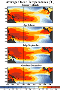
Average equatorial Pacific temperatures
If the temperature variation from climatology is within 0.5 °C (0.9 °F), ENSO conditions are described as neutral. Neutral conditions are the transition between warm and cold phases of ENSO. Ocean temperatures (by definition), tropical precipitation, and wind patterns are near average conditions during this phase.
[24] Close to half of all years are within neutral periods.
[25] During the neutral ENSO phase, other climate anomalies/patterns such as the sign of the
North Atlantic Oscillation or the
Pacific–North American teleconnection pattern exert more influence.
[26]
Warm phase
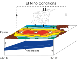
When the Walker circulation weakens or reverses and the
Hadley circulation strengthens an El Niño results,
[27] causing the ocean surface to be warmer than average, as upwelling of cold water occurs less or not at all offshore northwestern South America. El Niño (
,
,
Spanish pronunciation: [el ˈniɲo]) is associated with a band of warmer than average ocean water temperatures that periodically develops off the Pacific coast of South America.
El niño is
Spanish for "the boy", and the capitalized term El Niño refers to the
Christ child, Jesus, because periodic warming in the Pacific near
South America is usually noticed around
Christmas.
[28] It is a phase of 'El Niño–Southern Oscillation' (ENSO), which refers to variations in the temperature of the surface of the tropical eastern Pacific Ocean and in air
surface pressure in the tropical western Pacific. The warm oceanic phase, El Niño, accompanies high air surface pressure in the western Pacific.
[1][29] Mechanisms that cause the oscillation remain under study.
Cold phase
An especially strong Walker circulation causes a La Niña, resulting in cooler ocean temperatures due to increased upwelling. La Niña (
,
Spanish pronunciation: [la ˈniɲa]) is a coupled ocean-atmosphere phenomenon that is the counterpart of El Niño as part of the broader El Niño Southern Oscillation
climate pattern. The name La Niña originates from
Spanish, meaning "the girl", analogous to El Niño meaning "the boy". It has also in the past been called
anti-El Niño, and El Viejo (meaning "the old man").
[30] During a period of La Niña, the
sea surface temperature across the equatorial eastern central Pacific will be lower than normal by 3–5 °C. In the United States, an
appearance of La Niña happens for at least five months of La Niña conditions. La Niña, sometimes informally called "anti-El Niño", is the opposite of El Niño, with a sea surface temperature anomaly of at least 0.5 °C (0.9 °F) below normal and its effects are often the reverse of those of El Niño.
Impacts
On precipitation

Regional impacts of La Niña.
Developing countries dependent upon agriculture and fishing, particularly those bordering the Pacific Ocean, are the most affected by ENSO. The effects of El Niño in South America are direct and strong. An El Niño is associated with warm and very wet weather months in April–October along the coasts of northern
Peru and
Ecuador, causing major flooding whenever the event is strong or extreme.
[31] La Niña causes a drop in sea surface temperatures over Southeast Asia and heavy rains over
Malaysia, the
Philippines, and
Indonesia.
[32]
To the north across
Alaska, La Niña events lead to drier than normal conditions, while El Niño events do not have a correlation towards dry or wet conditions. During El Niño events, increased precipitation is expected in California due to a more southerly, zonal, storm track.
[33] During La Niña, increased precipitation is diverted into the
Pacific Northwest due to a more northerly storm track.
[34] During La Niña events, the storm track shifts far enough northward to bring wetter than normal winter conditions (in the form of increased snowfall) to the Midwestern states, as well as hot and dry summers.
[35] During the El Niño portion of
ENSO, increased precipitation falls along the Gulf coast and Southeast due to a stronger than normal, and more southerly,
polar jet stream.
[36] In the late winter and spring during El Niño events, drier than average conditions can be expected in Hawaii.
[37] On Guam during El Niño years, dry season precipitation averages below normal. However, the threat of a tropical cyclone is over triple what is normal during El Niño years, so extreme shorter duration rainfall events are possible.
[38] On American Samoa during El Niño events, precipitation averages about 10 percent above normal, while La Niña events lead to precipitation amounts which average close to 10 percent below normal.
[39] ENSO is linked to rainfall over Puerto Rico.
[40] During an El Niño, snowfall is greater than average across the southern Rockies and Sierra Nevada mountain range, and is well-below normal across the Upper Midwest and Great Lakes states. During a La Niña, snowfall is above normal across the Pacific Northwest and western Great Lakes.
[41]
On Tehuantepecers
The synoptic condition for the Tehuantepecer, a violent mountain-gap wind in between the mountains of
Mexico and
Guatemala, is associated with
high-pressure system forming in
Sierra Madre of Mexico in the wake of an advancing cold front, which causes winds to accelerate through the
Isthmus of Tehuantepec. Tehuantepecers primarily occur during the cold season months for the region in the wake of cold fronts, between October and February, with a summer maximum in July caused by the westward extension of the Azores-Bermuda high pressure system. Wind magnitude is greater during El Niño years than during La Niña years, due to the more frequent cold frontal incursions during El Niño winters.
[42] Tehuantepec winds reach 20 knots (40 km/h) to 45 knots (80 km/h), and on rare occasions 100 knots (200 km/h). The wind’s direction is from the north to north-northeast.
[43] It leads to a localized acceleration of the
trade winds in the region, and can enhance
thunderstorm activity when it interacts with the
Intertropical Convergence Zone.
[44] The effects can last from a few hours to six days.
[45]
On global warming

NOAA graph of Global Annual Temperature Anomalies 1950–2012, showing ENSO
During the last several decades, the number of El Niño events increased, and the number of La Niña events decreased,
[46] although observation of ENSO for much longer is needed to detect robust changes.
[47] The question is whether this is a random fluctuation or a normal instance of variation for that phenomenon or the result of global climate changes toward
global warming.
The studies of historical data show the recent El Niño variation is most likely linked to global warming. For example, one of the most recent results, even after subtracting the positive influence of decadal variation, is shown to be possibly present in the ENSO trend,
[48] the amplitude of the ENSO variability in the observed data still increases, by as much as 60% in the last 50 years.
[49]
The exact changes happening to ENSO in the future is uncertain:
[50] Different models make different predictions.
[51][52] It may be that the observed phenomenon of more frequent and stronger El Niño events occurs only in the initial phase of the global warming, and then (e.g., after the lower layers of the ocean get warmer, as well), El Niño will become weaker than it was.
[53] It may also be that the stabilizing and destabilizing forces influencing the phenomenon will eventually compensate for each other.
[54] More research is needed to provide a better answer to that question. The ENSO is considered to be a potential
tipping element in Earth's climate.
[55]
ENSO diversity
The traditional ENSO (El Niño Southern Oscillation), also called Eastern Pacific (EP) ENSO,
[56] involves temperature anomalies in the eastern pacific. However, in the 1990s and 2000s, nontraditional ENSO conditions were observed, in which the usual place of the temperature anomaly (Niño 1 and 2) is not affected, but an anomaly arises in the central Pacific (Niño 3.4).
[57] The phenomenon is called Central Pacific (CP) ENSO,
[56] "dateline" ENSO (because the anomaly arises near the
dateline), or ENSO "Modoki" (Modoki is
Japanese for "similar, but different").
[58][59] There are flavors of ENSO additional to EP and CP types and some scientists argue that ENSO exists as a continuum often with hybrid types.
[60]
The effects of the CP ENSO are different from those of the traditional EP ENSO. The
El Niño Modoki leads to more hurricanes more frequently making landfall in the Atlantic.
[61] La Niña Modoki leads to a rainfall increase over
northwestern Australia and northern
Murray-Darling basin, rather than over the east as in a conventional La Niña.
[59] Also, La Niña Modoki increases the frequency of cyclonic storms over
Bay of Bengal, but decreases the occurrence of severe storms in the
Indian Ocean.
[62]
The recent discovery of ENSO Modoki has some scientists believing it to be linked to global warming.
[63] However, comprehensive satellite data go back only to 1979. More research must be done to find the correlation and study past El Niño episodes. More generally, there is no scientific consensus on how/if
climate change may affect ENSO.
[50]
There is also a scientific debate on the very existence of this "new" ENSO. Indeed, a number of studies dispute the reality of this statistical distinction or its increasing occurrence, or both, either arguing the reliable record is too short to detect such a distinction,
[64][65] finding no distinction or trend using other statistical approaches,
[66][67][68][69][70] or that other types should be distinguished, such as standard and extreme ENSO.
[71][72] Following the asymmetric nature of the warm and cold phases of ENSO, some studies could not identify such distinctions for La Niña, both in observations and in the climate models,
[73] but some sources indicate that there is a variation on La Niña with cooler waters on central Pacific and average or warmer water temperatures on both eastern and western Pacific, also showing eastern Pacific ocean currents going to the opposite direction compared to the currents in traditional La Niñas.
[58][74][75]


 " and p is denoted "
 ".)
".)


