From Wikipedia, the free encyclopedia

An example of Beer–Lambert law: green laser light in a solution of Rhodamine 6B. The beam radiant power becomes weaker as it passes through solution
History
The law was discovered by Pierre Bouguer before 1729.[1] It is often attributed to Johann Heinrich Lambert, who cited Bouguer's Essai d'optique sur la gradation de la lumière (Claude Jombert, Paris, 1729)—and even quoted from it—in his Photometria in 1760.[2] Lambert's law stated that absorbance of a material sample is directly proportional to its thickness (path length). Much later, August Beer discovered another attenuation relation in 1852. Beer's law stated that absorbance is proportional to the concentrations of the attenuating species in the material sample in 1852.[3] The modern derivation of the Beer–Lambert law combines the two laws and correlates the absorbance to both the concentrations of the attenuating species as well as the thickness of the material sample.[4]Beer–Lambert law
By definition, the transmittance of material sample is related to its optical depth τ and to its absorbance A as
- Φet is the radiant flux transmitted by that material sample;
- Φei is the radiant flux received by that material sample.


- σi is the attenuation cross section of the attenuating species i in the material sample;
- ni is the number density of the attenuating species i in the material sample;
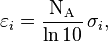
- εi is the molar attenuation coefficient of the attenuating species i in the material sample;
- ci is the amount concentration of the attenuating species i in the material sample;
- ℓ is the path length of the beam of light through the material sample.

In case of uniform attenuation, these relations become[5]


The law tends to break down at very high concentrations, especially if the material is highly scattering. If the radiation is especially intense, nonlinear optical processes can also cause variances. The main reason, however, is the following. At high concentrations, the molecules are closer to each other and begin to interact with each other. This interaction will change several properties of the molecule, and thus will change the attenuation.
Expression with attenuation coefficient
The Beer–Lambert law can be expressed in terms of attenuation coefficient, but in this case is better called Lambert's law since amount concentration, from Beer's law, is hidden inside the attenuation coefficient. The (Napierian) attenuation coefficient μ and the decadic attenuation coefficient μ10 = μ/ln 10 of a material sample are related to its number densities and amount concentrations as


Derivation
In concept, the derivation of the Beer–Lambert law is straightforward. Assume that a beam of light enters a material sample. Define z as an axis parallel to the direction of the beam. Divide the material sample into thin slices, perpendicular to the beam of light, with thickness dz sufficiently small that one particle in a slice cannot obscure another particle in the same slice when viewed along the z direction. The radiant flux of the light that emerges from a slice is reduced, compared to that of the light that entered, by dΦe(z) = −μ(z)Φe(z) dz, where μ is the (Napierian) attenuation coefficient, which yields the following first-order linear ODE:


Validity
Under certain conditions Beer–Lambert law fails to maintain a linear relationship between attenuation and concentration of analyte.[6] These deviations are classified into three categories:- Real—fundamental deviations due to the limitations of the law itself.
- Chemical—deviations observed due to specific chemical species of the sample which is being analyzed.
- Instrument—deviations which occur due to how the attenuation measurements are made.
- The attenuators must act independently of each other.
- The attenuating medium must be homogeneous in the interaction volume.
- The attenuating medium must not scatter the radiation—no turbidity—unless this is accounted for as in DOAS.
- The incident radiation must consist of parallel rays, each traversing the same length in the absorbing medium.
- The incident radiation should preferably be monochromatic, or have at least a width that is narrower than that of the attenuating transition. Otherwise a spectrometer as detector for the power is needed instead of a photodiode which has not a selective wavelength dependence.
- The incident flux must not influence the atoms or molecules; it should only act as a non-invasive probe of the species under study. In particular, this implies that the light should not cause optical saturation or optical pumping, since such effects will deplete the lower level and possibly give rise to stimulated emission.
Chemical analysis by spectrophotometry
Beer–Lambert law can be applied to the analysis of a mixture by spectrophotometry, without the need for extensive pre-processing of the sample. An example is the determination of bilirubin in blood plasma samples. The spectrum of pure bilirubin is known, so the molar attenuation coefficient ε is known. Measurements of decadic attenuation coefficient μ10 are made at one wavelength λ that is nearly unique for bilirubin and at a second wavelength in order to correct for possible interferences. The amount concentration c is then given by

The law is used widely in infra-red spectroscopy and near-infrared spectroscopy for analysis of polymer degradation and oxidation (also in biological tissue). The carbonyl group attenuation at about 6 micrometres can be detected quite easily, and degree of oxidation of the polymer calculated.
Beer–Lambert law in the atmosphere
This law is also applied to describe the attenuation of solar or stellar radiation as it travels through the atmosphere. In this case, there is scattering of radiation as well as absorption. The optical depth for a slant path is τ′ = mτ, where τ refers to a vertical path, m is called the relative airmass, and for a plane-parallel atmosphere it is determined as m = sec θ where θ is the zenith angle corresponding to the given path. The Beer–Lambert law for the atmosphere is usually written
- a refers to aerosols (that absorb and scatter);
- g are uniformly mixed gases (mainly carbon dioxide (CO2) and molecular oxygen (O2) which only absorb);
- NO2 is nitrogen dioxide, mainly due to urban pollution (absorption only);
- RS are effects due to Raman scattering in the atmosphere;
- w is water vapour absorption;
- O3 is ozone (absorption only);
- r is Rayleigh scattering from molecular oxygen (O2) and nitrogen (N2) (responsible for the blue color of the sky);
- the selection of the attenuators which have to be considered depends on the wavelength range and can include various other compounds. This can include tetraoxygen, HONO, formaldehyde, glyoxal, a series of halogen radicals and others.

 is the lapse rate given in
  or
or  can be used to represent the adiabatic lapse rate in order to avoid confusion with other terms symbolized by

 and :
and : we can show that:
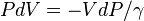
 is the specific heat at constant pressure and
 is the density. Combining these two equations to eliminate the pressure, one arrives at the result for the DALR,
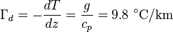


 , where


 is the elevation,
 is the
  is the pressure at a given point at elevation
  is pressure at the reference point = 101325 Pa at sea level.
 is the atmospheric lapse rate (change in temperature / distance) = -6.5e-3 K/m, and
 is the temperature at the same reference point for which


