Weather models use systems of differential equations based on the laws of physics, fluid motion, and chemistry, and use a coordinate system which divides the planet into a 3D grid. Winds, heat transfer, solar radiation, relative humidity, and surface hydrology
are calculated within each grid cell, and the interactions with
neighboring cells are used to calculate atmospheric properties in the
future.
Numerical weather prediction (NWP) uses mathematical models of the atmosphere and oceans to predict the weather based on current weather conditions. Though first attempted in the 1920s, it was not until the advent of computer simulation in the 1950s that numerical weather predictions produced realistic results. A number of global and regional forecast models are run in different countries worldwide, using current weather observations relayed from radiosondes, weather satellites and other observing systems as inputs.
Mathematical models based on the same physical principles can be used to generate either short-term weather forecasts or longer-term climate predictions; the latter are widely applied for understanding and projecting climate change. The improvements made to regional models have allowed for significant improvements in tropical cyclone track and air quality forecasts; however, atmospheric models perform poorly at handling processes that occur in a relatively constricted area, such as wildfires.
Manipulating the vast datasets and performing the complex calculations necessary to modern numerical weather prediction requires some of the most powerful supercomputers in the world. Even with the increasing power of supercomputers, the forecast skill of numerical weather models extends to only about six days. Factors affecting the accuracy of numerical predictions include the density and quality of observations used as input to the forecasts, along with deficiencies in the numerical models themselves. Post-processing techniques such as model output statistics (MOS) have been developed to improve the handling of errors in numerical predictions.
A more fundamental problem lies in the chaotic nature of the partial differential equations that govern the atmosphere. It is impossible to solve these equations exactly, and small errors grow with time (doubling about every five days). Present understanding is that this chaotic behavior limits accurate forecasts to about 14 days even with perfectly accurate input data and a flawless model. In addition, the partial differential equations used in the model need to be supplemented with parameterizations for solar radiation, moist processes (clouds and precipitation), heat exchange, soil, vegetation, surface water, and the effects of terrain. In an effort to quantify the large amount of inherent uncertainty remaining in numerical predictions, ensemble forecasts have been used since the 1990s to help gauge the confidence in the forecast, and to obtain useful results farther into the future than otherwise possible. This approach analyzes multiple forecasts created with an individual forecast model or multiple models.
History

The ENIAC main control panel at the Moore School of Electrical Engineering operated by Betty Jennings and Frances Bilas.
The history of numerical weather prediction began in the 1920s through the efforts of Lewis Fry Richardson, who used procedures originally developed by Vilhelm Bjerknes[1] to produce by hand a six-hour forecast for the state of the atmosphere over two points in central Europe, taking at least six weeks to do so.[1][2] It was not until the advent of the computer and computer simulations that computation time was reduced to less than the forecast period itself. The ENIAC was used to create the first weather forecasts via computer in 1950, based on a highly simplified approximation to the atmospheric governing equations.[3][4] In 1954, Carl-Gustav Rossby's group at the Swedish Meteorological and Hydrological Institute used the same model to produce the first operational forecast (i.e., a routine prediction for practical use).[5] Operational numerical weather prediction in the United States began in 1955 under the Joint Numerical Weather Prediction Unit (JNWPU), a joint project by the U.S. Air Force, Navy and Weather Bureau.[6] In 1956, Norman Phillips developed a mathematical model which could realistically depict monthly and seasonal patterns in the troposphere; this became the first successful climate model.[7][8] Following Phillips' work, several groups began working to create general circulation models.[9] The first general circulation climate model that combined both oceanic and atmospheric processes was developed in the late 1960s at the NOAA Geophysical Fluid Dynamics Laboratory.[10]
As computers have become more powerful, the size of the initial data sets has increased and newer atmospheric models have been developed to take advantage of the added available computing power. These newer models include more physical processes in the simplifications of the equations of motion in numerical simulations of the atmosphere.[5] In 1966, West Germany and the United States began producing operational forecasts based on primitive-equation models, followed by the United Kingdom in 1972 and Australia in 1977.[1][11] The development of limited area (regional) models facilitated advances in forecasting the tracks of tropical cyclones as well as air quality in the 1970s and 1980s.[12][13] By the early 1980s models began to include the interactions of soil and vegetation with the atmosphere, which led to more realistic forecasts.[14]
The output of forecast models based on atmospheric dynamics is unable to resolve some details of the weather near the Earth's surface. As such, a statistical relationship between the output of a numerical weather model and the ensuing conditions at the ground was developed in the 1970s and 1980s, known as model output statistics (MOS).[15][16] Starting in the 1990s, model ensemble forecasts have been used to help define the forecast uncertainty and to extend the window in which numerical weather forecasting is viable farther into the future than otherwise possible.[17][18][19]
Initialization

Weather reconnaissance aircraft, such as this WP-3D Orion, provide data that is then used in numerical weather forecasts.
The atmosphere is a fluid. As such, the idea of numerical weather prediction is to sample the state of the fluid at a given time and use the equations of fluid dynamics and thermodynamics to estimate the state of the fluid at some time in the future. The process of entering observation data into the model to generate initial conditions is called initialization. On land, terrain maps available at resolutions down to 1 kilometer (0.6 mi) globally are used to help model atmospheric circulations within regions of rugged topography, in order to better depict features such as downslope winds, mountain waves and related cloudiness that affects incoming solar radiation.[20] The main inputs from country-based weather services are observations from devices (called radiosondes) in weather balloons that measure various atmospheric parameters and transmits them to a fixed receiver, as well as from weather satellites. The World Meteorological Organization acts to standardize the instrumentation, observing practices and timing of these observations worldwide. Stations either report hourly in METAR reports,[21] or every six hours in SYNOP reports.[22] These observations are irregularly spaced, so they are processed by data assimilation and objective analysis methods, which perform quality control and obtain values at locations usable by the model's mathematical algorithms.[23] The data are then used in the model as the starting point for a forecast.[24]
A variety of methods are used to gather observational data for use in numerical models. Sites launch radiosondes in weather balloons which rise through the troposphere and well into the stratosphere.[25] Information from weather satellites is used where traditional data sources are not available. Commerce provides pilot reports along aircraft routes[26] and ship reports along shipping routes.[27] Research projects use reconnaissance aircraft to fly in and around weather systems of interest, such as tropical cyclones.[28][29] Reconnaissance aircraft are also flown over the open oceans during the cold season into systems which cause significant uncertainty in forecast guidance, or are expected to be of high impact from three to seven days into the future over the downstream continent.[30] Sea ice began to be initialized in forecast models in 1971.[31] Efforts to involve sea surface temperature in model initialization began in 1972 due to its role in modulating weather in higher latitudes of the Pacific.[32]
Computation

A prognostic chart of the 96-hour forecast of 850 mbar geopotential height and temperature from the Global Forecast System
An atmospheric model is a computer program that produces meteorological information for future times at given locations and altitudes. Within any modern model is a set of equations, known as the primitive equations, used to predict the future state of the atmosphere.[33] These equations—along with the ideal gas law—are used to evolve the density, pressure, and potential temperature scalar fields and the air velocity (wind) vector field of the atmosphere through time. Additional transport equations for pollutants and other aerosols are included in some primitive-equation high-resolution models as well.[34] The equations used are nonlinear partial differential equations which are impossible to solve exactly through analytical methods,[35] with the exception of a few idealized cases.[36] Therefore, numerical methods obtain approximate solutions. Different models use different solution methods: some global models and almost all regional models use finite difference methods for all three spatial dimensions, while other global models and a few regional models use spectral methods for the horizontal dimensions and finite-difference methods in the vertical.[35]
These equations are initialized from the analysis data and rates of change are determined. These rates of change predict the state of the atmosphere a short time into the future; the time increment for this prediction is called a time step. This future atmospheric state is then used as the starting point for another application of the predictive equations to find new rates of change, and these new rates of change predict the atmosphere at a yet further time step into the future. This time stepping is repeated until the solution reaches the desired forecast time. The length of the time step chosen within the model is related to the distance between the points on the computational grid, and is chosen to maintain numerical stability.[37] Time steps for global models are on the order of tens of minutes,[38] while time steps for regional models are between one and four minutes.[39] The global models are run at varying times into the future. The UKMET Unified Model is run six days into the future,[40] while the European Centre for Medium-Range Weather Forecasts' Integrated Forecast System and Environment Canada's Global Environmental Multiscale Model both run out to ten days into the future,[41] and the Global Forecast System model run by the Environmental Modeling Center is run sixteen days into the future.[42] The visual output produced by a model solution is known as a prognostic chart, or prog.[43]
Parameterization

Field of cumulus clouds, which are parameterized since they are too small to be explicitly included within numerical weather prediction
Some meteorological processes are too small-scale or too complex to be explicitly included in numerical weather prediction models. Parameterization is a procedure for representing these processes by relating them to variables on the scales that the model resolves. For example, the gridboxes in weather and climate models have sides that are between 5 kilometers (3 mi) and 300 kilometers (200 mi) in length. A typical cumulus cloud has a scale of less than 1 kilometer (0.6 mi), and would require a grid even finer than this to be represented physically by the equations of fluid motion. Therefore, the processes that such clouds represent are parameterized, by processes of various sophistication. In the earliest models, if a column of air within a model gridbox was conditionally unstable (essentially, the bottom was warmer and moister than the top) and the water vapor content at any point within the column became saturated then it would be overturned (the warm, moist air would begin rising), and the air in that vertical column mixed. More sophisticated schemes recognize that only some portions of the box might convect and that entrainment and other processes occur. Weather models that have gridboxes with sides between 5 and 25 kilometers (3 and 16 mi) can explicitly represent convective clouds, although they need to parameterize cloud microphysics which occur at a smaller scale.[44] The formation of large-scale (stratus-type) clouds is more physically based; they form when the relative humidity reaches some prescribed value. Sub-grid scale processes need to be taken into account. Rather than assuming that clouds form at 100% relative humidity, the cloud fraction can be related to a critical value of relative humidity less than 100%,[45] reflecting the sub grid scale variation that occurs in the real world.
The amount of solar radiation reaching the ground, as well as the formation of cloud droplets occur on the molecular scale, and so they must be parameterized before they can be included in the model. Atmospheric drag produced by mountains must also be parameterized, as the limitations in the resolution of elevation contours produce significant underestimates of the drag.[46] This method of parameterization is also done for the surface flux of energy between the ocean and the atmosphere, in order to determine realistic sea surface temperatures and type of sea ice found near the ocean's surface.[47] Sun angle as well as the impact of multiple cloud layers is taken into account.[48] Soil type, vegetation type, and soil moisture all determine how much radiation goes into warming and how much moisture is drawn up into the adjacent atmosphere, and thus it is important to parameterize their contribution to these processes.[49] Within air quality models, parameterizations take into account atmospheric emissions from multiple relatively tiny sources (e.g. roads, fields, factories) within specific grid boxes.[50]
Domains

A cross-section of the atmosphere over terrain with a sigma-coordinate
representation shown. Mesoscale models divide the atmosphere vertically
using representations similar to the one shown here.
The horizontal domain of a model is either global, covering the entire Earth, or regional, covering only part of the Earth. Regional models (also known as limited-area models, or LAMs) allow for the use of finer grid spacing than global models because the available computational resources are focused on a specific area instead of being spread over the globe. This allows regional models to resolve explicitly smaller-scale meteorological phenomena that cannot be represented on the coarser grid of a global model. Regional models use a global model to specify conditions at the edge of their domain (boundary conditions) in order to allow systems from outside the regional model domain to move into its area. Uncertainty and errors within regional models are introduced by the global model used for the boundary conditions of the edge of the regional model, as well as errors attributable to the regional model itself.[51]
Coordinate systems
Horizontal coordinates
Horizontal position may be expressed directly in geographic coordinates (latitude and longitude) for global models or in a map projection planar coordinates for regional models.Vertical coordinates
The vertical coordinate is handled in various ways. Lewis Fry Richardson's 1922 model used geometric height ( ) as the vertical coordinate. Later models substituted the geometric coordinate with a pressure coordinate system, in which the geopotential heights of constant-pressure surfaces become dependent variables, greatly simplifying the primitive equations.[52] This correlation between coordinate systems can be made since pressure decreases with height through the Earth's atmosphere.[53]
The first model used for operational forecasts, the single-layer
barotropic model, used a single pressure coordinate at the 500-millibar
(about 5,500 m (18,000 ft)) level,[3] and thus was essentially two-dimensional. High-resolution models—also called mesoscale models—such as the Weather Research and Forecasting model tend to use normalized pressure coordinates referred to as sigma coordinates.[54] This coordinate system receives its name from the independent variable
) as the vertical coordinate. Later models substituted the geometric coordinate with a pressure coordinate system, in which the geopotential heights of constant-pressure surfaces become dependent variables, greatly simplifying the primitive equations.[52] This correlation between coordinate systems can be made since pressure decreases with height through the Earth's atmosphere.[53]
The first model used for operational forecasts, the single-layer
barotropic model, used a single pressure coordinate at the 500-millibar
(about 5,500 m (18,000 ft)) level,[3] and thus was essentially two-dimensional. High-resolution models—also called mesoscale models—such as the Weather Research and Forecasting model tend to use normalized pressure coordinates referred to as sigma coordinates.[54] This coordinate system receives its name from the independent variable  used to scale
atmospheric pressures with respect to the pressure at the surface, and
in some cases also with the pressure at the top of the domain.[55]
used to scale
atmospheric pressures with respect to the pressure at the surface, and
in some cases also with the pressure at the top of the domain.[55]Model output statistics
Because forecast models based upon the equations for atmospheric dynamics do not perfectly determine weather conditions, statistical methods have been developed to attempt to correct the forecasts. Statistical models were created based upon the three-dimensional fields produced by numerical weather models, surface observations and the climatological conditions for specific locations. These statistical models are collectively referred to as model output statistics (MOS),[56] and were developed by the National Weather Service for their suite of weather forecasting models in the late 1960s.[15][57]Model output statistics differ from the perfect prog technique, which assumes that the output of numerical weather prediction guidance is perfect.[58] MOS can correct for local effects that cannot be resolved by the model due to insufficient grid resolution, as well as model biases. Because MOS is run after its respective global or regional model, its production is known as post-processing. Forecast parameters within MOS include maximum and minimum temperatures, percentage chance of rain within a several hour period, precipitation amount expected, chance that the precipitation will be frozen in nature, chance for thunderstorms, cloudiness, and surface winds.[59]
Ensembles

Top: Weather Research and Forecasting model (WRF) simulation of Hurricane Rita (2005) tracks. Bottom: The spread of NHC multi-model ensemble forecast.
In 1963, Edward Lorenz discovered the chaotic nature of the fluid dynamics equations involved in weather forecasting.[60] Extremely small errors in temperature, winds, or other initial inputs given to numerical models will amplify and double every five days,[60] making it impossible for long-range forecasts—those made more than two weeks in advance—to predict the state of the atmosphere with any degree of forecast skill. Furthermore, existing observation networks have poor coverage in some regions (for example, over large bodies of water such as the Pacific Ocean), which introduces uncertainty into the true initial state of the atmosphere. While a set of equations, known as the Liouville equations, exists to determine the initial uncertainty in the model initialization, the equations are too complex to run in real-time, even with the use of supercomputers.[61] These uncertainties limit forecast model accuracy to about five or six days into the future.[62][63]
Edward Epstein recognized in 1969 that the atmosphere could not be completely described with a single forecast run due to inherent uncertainty, and proposed using an ensemble of stochastic Monte Carlo simulations to produce means and variances for the state of the atmosphere.[64] Although this early example of an ensemble showed skill, in 1974 Cecil Leith showed that they produced adequate forecasts only when the ensemble probability distribution was a representative sample of the probability distribution in the atmosphere.[65]
Since the 1990s, ensemble forecasts have been used operationally (as routine forecasts) to account for the stochastic nature of weather processes – that is, to resolve their inherent uncertainty. This method involves analyzing multiple forecasts created with an individual forecast model by using different physical parametrizations or varying initial conditions.[61] Starting in 1992 with ensemble forecasts prepared by the European Centre for Medium-Range Weather Forecasts (ECMWF) and the National Centers for Environmental Prediction, model ensemble forecasts have been used to help define the forecast uncertainty and to extend the window in which numerical weather forecasting is viable farther into the future than otherwise possible.[17][18][19] The ECMWF model, the Ensemble Prediction System,[18] uses singular vectors to simulate the initial probability density, while the NCEP ensemble, the Global Ensemble Forecasting System, uses a technique known as vector breeding.[17][19] The UK Met Office runs global and regional ensemble forecasts where perturbations to initial conditions are produced using a Kalman filter.[66] There are 24 ensemble members in the Met Office Global and Regional Ensemble Prediction System (MOGREPS).
In a single model-based approach, the ensemble forecast is usually evaluated in terms of an average of the individual forecasts concerning one forecast variable, as well as the degree of agreement between various forecasts within the ensemble system, as represented by their overall spread. Ensemble spread is diagnosed through tools such as spaghetti diagrams, which show the dispersion of one quantity on prognostic charts for specific time steps in the future. Another tool where ensemble spread is used is a meteogram, which shows the dispersion in the forecast of one quantity for one specific location. It is common for the ensemble spread to be too small to include the weather that actually occurs, which can lead to forecasters misdiagnosing model uncertainty;[67] this problem becomes particularly severe for forecasts of the weather about ten days in advance.[68] When ensemble spread is small and the forecast solutions are consistent within multiple model runs, forecasters perceive more confidence in the ensemble mean, and the forecast in general.[67] Despite this perception, a spread-skill relationship is often weak or not found, as spread-error correlations are normally less than 0.6, and only under special circumstances range between 0.6–0.7.[69] The relationship between ensemble spread and forecast skill varies substantially depending on such factors as the forecast model and the region for which the forecast is made.
In the same way that many forecasts from a single model can be used to form an ensemble, multiple models may also be combined to produce an ensemble forecast. This approach is called multi-model ensemble forecasting, and it has been shown to improve forecasts when compared to a single model-based approach.[70] Models within a multi-model ensemble can be adjusted for their various biases, which is a process known as superensemble forecasting. This type of forecast significantly reduces errors in model output.[71]
Applications
Air quality modeling
Air quality forecasting attempts to predict when the concentrations of pollutants will attain levels that are hazardous to public health. The concentration of pollutants in the atmosphere is determined by their transport, or mean velocity of movement through the atmosphere, their diffusion, chemical transformation, and ground deposition.[72] In addition to pollutant source and terrain information, these models require data about the state of the fluid flow in the atmosphere to determine its transport and diffusion.[73] Meteorological conditions such as thermal inversions can prevent surface air from rising, trapping pollutants near the surface,[74] which makes accurate forecasts of such events crucial for air quality modeling. Urban air quality models require a very fine computational mesh, requiring the use of high-resolution mesoscale weather models; in spite of this, the quality of numerical weather guidance is the main uncertainty in air quality forecasts.[73]Climate modeling
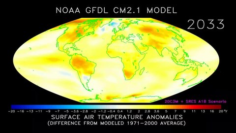
A General Circulation Model (GCM) is a mathematical model that can be used in computer simulations of the global circulation of a planetary atmosphere or ocean. An atmospheric general circulation model (AGCM) is essentially the same as a global numerical weather prediction model, and some (such as the one used in the UK Unified Model) can be configured for both short-term weather forecasts and longer-term climate predictions. Along with sea ice and land-surface components, AGCMs and oceanic GCMs (OGCM) are key components of global climate models, and are widely applied for understanding the climate and projecting climate change. For aspects of climate change, a range of man-made chemical emission scenarios can be fed into the climate models to see how an enhanced greenhouse effect would modify the Earth's climate.[75] Versions designed for climate applications with time scales of decades to centuries were originally created in 1969 by Syukuro Manabe and Kirk Bryan at the Geophysical Fluid Dynamics Laboratory in Princeton, New Jersey.[76] When run for multiple decades, computational limitations mean that the models must use a coarse grid that leaves smaller-scale interactions unresolved.[77]Ocean surface modeling

NOAA Wavewatch III 120-hour wind and wave forecast for the North Atlantic
The transfer of energy between the wind blowing over the surface of an ocean and the ocean's upper layer is an important element in wave dynamics.[78] The spectral wave transport equation is used to describe the change in wave spectrum over changing topography. It simulates wave generation, wave movement (propagation within a fluid), wave shoaling, refraction, energy transfer between waves, and wave dissipation.[79] Since surface winds are the primary forcing mechanism in the spectral wave transport equation, ocean wave models use information produced by numerical weather prediction models as inputs to determine how much energy is transferred from the atmosphere into the layer at the surface of the ocean. Along with dissipation of energy through whitecaps and resonance between waves, surface winds from numerical weather models allow for more accurate predictions of the state of the sea surface.[80]
Tropical cyclone forecasting
Tropical cyclone forecasting also relies on data provided by numerical weather models. Three main classes of tropical cyclone guidance models exist: Statistical models are based on an analysis of storm behavior using climatology, and correlate a storm's position and date to produce a forecast that is not based on the physics of the atmosphere at the time. Dynamical models are numerical models that solve the governing equations of fluid flow in the atmosphere; they are based on the same principles as other limited-area numerical weather prediction models but may include special computational techniques such as refined spatial domains that move along with the cyclone. Models that use elements of both approaches are called statistical-dynamical models.[81]In 1978, the first hurricane-tracking model based on atmospheric dynamics—the movable fine-mesh (MFM) model—began operating.[12] Within the field of tropical cyclone track forecasting, despite the ever-improving dynamical model guidance which occurred with increased computational power, it was not until the 1980s when numerical weather prediction showed skill, and until the 1990s when it consistently outperformed statistical or simple dynamical models.[82] Predictions of the intensity of a tropical cyclone based on numerical weather prediction continue to be a challenge, since statistical methods continue to show higher skill over dynamical guidance.[83]
Wildfire modeling
.svg)
A simple wildfire propagation model
On a molecular scale, there are two main competing reaction processes involved in the degradation of cellulose, or wood fuels, in wildfires. When there is a low amount of moisture in a cellulose fiber, volatilization of the fuel occurs; this process will generate intermediate gaseous products that will ultimately be the source of combustion. When moisture is present—or when enough heat is being carried away from the fiber, charring occurs. The chemical kinetics of both reactions indicate that there is a point at which the level of moisture is low enough—and/or heating rates high enough—for combustion processes become self-sufficient. Consequently, changes in wind speed, direction, moisture, temperature, or lapse rate at different levels of the atmosphere can have a significant impact on the behavior and growth of a wildfire. Since the wildfire acts as a heat source to the atmospheric flow, the wildfire can modify local advection patterns, introducing a feedback loop between the fire and the atmosphere.[84]
A simplified two-dimensional model for the spread of wildfires that used convection to represent the effects of wind and terrain, as well as radiative heat transfer as the dominant method of heat transport led to reaction-diffusion systems of partial differential equations.[85][86] More complex models join numerical weather models or computational fluid dynamics models with a wildfire component which allow the feedback effects between the fire and the atmosphere to be estimated.[84] The additional complexity in the latter class of models translates to a corresponding increase in their computer power requirements. In fact, a full three-dimensional treatment of combustion via direct numerical simulation at scales relevant for atmospheric modeling is not currently practical because of the excessive computational cost such a simulation would require. Numerical weather models have limited forecast skill at spatial resolutions under 1 kilometer (0.6 mi), forcing complex wildfire models to parameterize the fire in order to calculate how the winds will be modified locally by the wildfire, and to use those modified winds to determine the rate at which the fire will spread locally.[87][88][89] Although models such as Los Alamos' FIRETEC solve for the concentrations of fuel and oxygen, the computational grid cannot be fine enough to resolve the combustion reaction, so approximations must be made for the temperature distribution within each grid cell, as well as for the combustion reaction rates themselves.