Positive feedback

From Wikipedia, the free encyclopedia
https://en.wikipedia.org/wiki/Positive_feedback

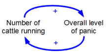
Alarm or panic can sometimes be spread by positive feedback among a herd of animals to cause a stampede.

 

Causal loop diagram that depicts the causes of a stampede as a positive feedback loop

 

In sociology a network effect can quickly create the positive feedback of a bank run. The above photo is of the UK Northern Rock 2007 bank run.

Positive feedback (exacerbating feedback, self-reinforcing feedback) is a process that occurs in a feedback loop which exacerbates the effects of a small disturbance. That is, the effects of a perturbation on a system include an increase in the magnitude of the perturbation. That is, A produces more of B which in turn produces more of A. In contrast, a system in which the results of a change act to reduce or counteract it has negative feedback. Both concepts play an important role in science and engineering, including biology, chemistry, and cybernetics.

Mathematically, positive feedback is defined as a positive loop gain around a closed loop of cause and effect. That is, positive feedback is in phase with the input, in the sense that it adds to make the input larger. Positive feedback tends to cause system instability. When the loop gain is positive and above 1, there will typically be exponential growth, increasing oscillations, chaotic behavior or other divergences from equilibrium. System parameters will typically accelerate towards extreme values, which may damage or destroy the system, or may end with the system latched into a new stable state. Positive feedback may be controlled by signals in the system being filtered, damped, or limited, or it can be cancelled or reduced by adding negative feedback.

Positive feedback is used in digital electronics to force voltages away from intermediate voltages into '0' and '1' states. On the other hand, thermal runaway is a type of positive feedback that can destroy semiconductor junctions. Positive feedback in chemical reactions can increase the rate of reactions, and in some cases can lead to explosions. Positive feedback in mechanical design causes tipping-point, or 'over-centre', mechanisms to snap into position, for example in switches and locking pliers. Out of control, it can cause bridges to collapse. Positive feedback in economic systems can cause boom-then-bust cycles. A familiar example of positive feedback is the loud squealing or howling sound produced by audio feedback in public address systems: the microphone picks up sound from its own loudspeakers, amplifies it, and sends it through the speakers again.

Platelet clotting demonstrates positive feedback. The damaged blood vessel wall releases chemicals that initiate the formation of a blood clot through platelet congregation. As more platelets gather, more chemicals are released that speed up the process. The process gets faster and faster until the blood vessel wall is completely sealed and the positive feedback loop has ended. The exponential form of the graph illustrates the positive feedback mechanism.

Overview

Positive feedback enhances or amplifies an effect by it having an influence on the process which gave rise to it. For example, when part of an electronic output signal returns to the input, and is in phase with it, the system gain is increased. The feedback from the outcome to the originating process can be direct, or it can be via other state variables. Such systems can give rich qualitative behaviors, but whether the feedback is instantaneously positive or negative in sign has an extremely important influence on the results. Positive feedback reinforces and negative feedback moderates the original process. Positive and negative in this sense refer to loop gains greater than or less than zero, and do not imply any value judgements as to the desirability of the outcomes or effects. A key feature of positive feedback is thus that small disturbances get bigger. When a change occurs in a system, positive feedback causes further change, in the same direction.

Basic

A basic feedback system can be represented by this block diagram. In the diagram the + symbol is an adder and A and B are arbitrary causal functions.

A simple feedback loop is shown in the diagram. If the loop gain AB is positive, then a condition of positive or regenerative feedback exists.

If the functions A and B are linear and AB is smaller than unity, then the overall system gain from the input to output is finite, but can be very large as AB approaches unity. In that case, it can be shown that the overall or "closed loop" gain from input to output is:

${\displaystyle G_{c}=A/(1-AB)}$

When AB > 1, the system is unstable, so does not have a well-defined gain; the gain may be called infinite.

Thus depending on the feedback, state changes can be convergent, or divergent. The result of positive feedback is to augment changes, so that small perturbations may result in big changes.

A system in equilibrium in which there is positive feedback to any change from its current state may be unstable, in which case the system is said to be in an unstable equilibrium. The magnitude of the forces that act to move such a system away from its equilibrium are an increasing function of the "distance" of the state from the equilibrium.

Positive feedback does not necessarily imply instability of an equilibrium, for example stable on and off states may exist in positive-feedback architectures.

Hysteresis

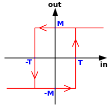
Hysteresis causes the output value to depend on the history of the input

 

In a Schmitt trigger circuit, feedback to the non-inverting input of an amplifier pushes the output directly away from the applied voltage towards the maximum or minimum voltage the amplifier can generate.

In the real world, positive feedback loops typically do not cause ever-increasing growth, but are modified by limiting effects of some sort. According to Donella Meadows:

"Positive feedback loops are sources of growth, explosion, erosion, and collapse in systems. A system with an unchecked positive loop ultimately will destroy itself. That’s why there are so few of them. Usually a negative loop will kick in sooner or later."

Hysteresis, in which the starting point affects where the system ends up, can be generated by positive feedback. When the gain of the feedback loop is above 1, then the output moves away from the input: if it is above the input, then it moves towards the nearest positive limit, while if it is below the input then it moves towards the nearest negative limit.

Once it reaches the limit, it will be stable. However, if the input goes past the limit, then the feedback will change sign and the output will move in the opposite direction until it hits the opposite limit. The system therefore shows bistable behaviour.

Terminology

The terms positive and negative were first applied to feedback before World War II. The idea of positive feedback was already current in the 1920s with the introduction of the regenerative circuit.

Friis & Jensen (1924) described regeneration in a set of electronic amplifiers as a case where the "feed-back" action is positive in contrast to negative feed-back action, which they mention only in passing. Harold Stephen Black's classic 1934 paper first details the use of negative feedback in electronic amplifiers. According to Black:

"Positive feed-back increases the gain of the amplifier, negative feed-back reduces it."

According to Mindell (2002) confusion in the terms arose shortly after this:

"...Friis and Jensen had made the same distinction Black used between 'positive feed-back' and 'negative feed-back', based not on the sign of the feedback itself but rather on its effect on the amplifier’s gain. In contrast, Nyquist and Bode, when they built on Black’s work, referred to negative feedback as that with the sign reversed. Black had trouble convincing others of the utility of his invention in part because confusion existed over basic matters of definition."

Examples and applications

In electronics

A vintage style regenerative radio receiver. Due to the controlled use of positive feedback, sufficient amplification can be derived from a single vacuum tube or valve (centre).

Regenerative circuits were invented and patented in 1914 for the amplification and reception of very weak radio signals. Carefully controlled positive feedback around a single transistor amplifier can multiply its gain by 1,000 or more. Therefore, a signal can be amplified 20,000 or even 100,000 times in one stage, that would normally have a gain of only 20 to 50. The problem with regenerative amplifiers working at these very high gains is that they easily become unstable and start to oscillate. The radio operator has to be prepared to tweak the amount of feedback fairly continuously for good reception. Modern radio receivers use the superheterodyne design, with many more amplification stages, but much more stable operation and no positive feedback.

The oscillation that can break out in a regenerative radio circuit is used in electronic oscillators. By the use of tuned circuits or a piezoelectric crystal (commonly quartz), the signal that is amplified by the positive feedback remains linear and sinusoidal. There are several designs for such harmonic oscillators, including the Armstrong oscillator, Hartley oscillator, Colpitts oscillator, and the Wien bridge oscillator. They all use positive feedback to create oscillations.

Many electronic circuits, especially amplifiers, incorporate negative feedback. This reduces their gain, but improves their linearity, input impedance, output impedance, and bandwidth, and stabilises all of these parameters, including the closed-loop gain. These parameters also become less dependent on the details of the amplifying device itself, and more dependent on the feedback components, which are less likely to vary with manufacturing tolerance, age and temperature. The difference between positive and negative feedback for AC signals is one of phase: if the signal is fed back out of phase, the feedback is negative and if it is in phase the feedback is positive. One problem for amplifier designers who use negative feedback is that some of the components of the circuit will introduce phase shift in the feedback path. If there is a frequency (usually a high frequency) where the phase shift reaches 180°, then the designer must ensure that the amplifier gain at that frequency is very low (usually by low-pass filtering). If the loop gain (the product of the amplifier gain and the extent of the positive feedback) at any frequency is greater than one, then the amplifier will oscillate at that frequency (Barkhausen stability criterion). Such oscillations are sometimes called parasitic oscillations. An amplifier that is stable in one set of conditions can break into parasitic oscillation in another. This may be due to changes in temperature, supply voltage, adjustment of front-panel controls, or even the proximity of a person or other conductive item.

Amplifiers may oscillate gently in ways that are hard to detect without an oscilloscope, or the oscillations may be so extensive that only a very distorted or no required signal at all gets through, or that damage occurs. Low frequency parasitic oscillations have been called 'motorboating' due to the similarity to the sound of a low-revving exhaust note.

 

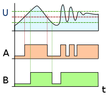
The effect of using a Schmitt trigger (B) instead of a comparator (A)

Many common digital electronic circuits employ positive feedback. While normal simple boolean logic gates usually rely simply on gain to push digital signal voltages away from intermediate values to the values that are meant to represent boolean '0' and '1', but many more complex gates use feedback. When an input voltage is expected to vary in an analogue way, but sharp thresholds are required for later digital processing, the Schmitt trigger circuit uses positive feedback to ensure that if the input voltage creeps gently above the threshold, the output is forced smartly and rapidly from one logic state to the other. One of the corollaries of the Schmitt trigger's use of positive feedback is that, should the input voltage move gently down again past the same threshold, the positive feedback will hold the output in the same state with no change. This effect is called hysteresis: the input voltage has to drop past a different, lower threshold to 'un-latch' the output and reset it to its original digital value. By reducing the extent of the positive feedback, the hysteresis-width can be reduced, but it can not entirely be eradicated. The Schmitt trigger is, to some extent, a latching circuit.

Positive feedback is a mechanism by which an output is enhanced, such as protein levels. However, in order to avoid any fluctuation in the protein level, the mechanism is inhibited stochastically (I), therefore when the concentration of the activated protein (A) is past the threshold ([I]), the loop mechanism is activated and the concentration of A increases exponentially if d[A]=k [A]

 

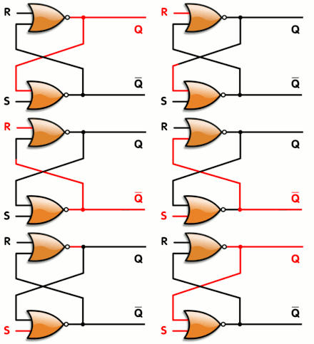
Illustration of an R-S ('reset-set') flip-flop made from two digital nor gates with positive feedback. Red and black mean logical '1' and '0', respectively.

An electronic flip-flop, or "latch", or "bistable multivibrator", is a circuit that due to high positive feedback is not stable in a balanced or intermediate state. Such a bistable circuit is the basis of one bit of electronic memory. The flip-flop uses a pair of amplifiers, transistors, or logic gates connected to each other so that positive feedback maintains the state of the circuit in one of two unbalanced stable states after the input signal has been removed, until a suitable alternative signal is applied to change the state. Computer random access memory (RAM) can be made in this way, with one latching circuit for each bit of memory.

Thermal runaway occurs in electronic systems because some aspect of a circuit is allowed to pass more current when it gets hotter, then the hotter it gets, the more current it passes, which heats it some more and so it passes yet more current. The effects are usually catastrophic for the device in question. If devices have to be used near to their maximum power-handling capacity, and thermal runaway is possible or likely under certain conditions, improvements can usually be achieved by careful design.

A phonograph turntable is prone to acoustic feedback.

Audio and video systems can demonstrate positive feedback. If a microphone picks up the amplified sound output of loudspeakers in the same circuit, then howling and screeching sounds of audio feedback (at up to the maximum power capacity of the amplifier) will be heard, as random noise is re-amplified by positive feedback and filtered by the characteristics of the audio system and the room.

Audio and live music

Audio feedback (also known as acoustic feedback, simply as feedback, or the Larsen effect) is a special kind of positive feedback which occurs when a sound loop exists between an audio input (for example, a microphone or guitar pickup) and an audio output (for example, a loudly-amplified loudspeaker). In this example, a signal received by the microphone is amplified and passed out of the loudspeaker. The sound from the loudspeaker can then be received by the microphone again, amplified further, and then passed out through the loudspeaker again. The frequency of the resulting sound is determined by resonance frequencies in the microphone, amplifier, and loudspeaker, the acoustics of the room, the directional pick-up and emission patterns of the microphone and loudspeaker, and the distance between them. For small PA systems the sound is readily recognized as a loud squeal or screech.

Feedback is almost always considered undesirable when it occurs with a singer's or public speaker's microphone at an event using a sound reinforcement system or PA system. Audio engineers use various electronic devices, such as equalizers and, since the 1990s, automatic feedback detection devices to prevent these unwanted squeals or screeching sounds, which detract from the audience's enjoyment of the event. On the other hand, since the 1960s, electric guitar players in rock music bands using loud guitar amplifiers and distortion effects have intentionally created guitar feedback to create a desirable musical effect. "I Feel Fine" by the Beatles marks one of the earliest examples of the use of feedback as a recording effect in popular music. It starts with a single, percussive feedback note produced by plucking the A string on Lennon's guitar. Artists such as the Kinks and the Who had already used feedback live, but Lennon remained proud of the fact that the Beatles were perhaps the first group to deliberately put it on vinyl. In one of his last interviews, he said, "I defy anybody to find a record—unless it's some old blues record in 1922—that uses feedback that way."

The principles of audio feedback were first discovered by Danish scientist Søren Absalon Larsen. Microphones are not the only transducers subject to this effect. Record deck pickup cartridges can do the same, usually in the low frequency range below about 100 Hz, manifesting as a low rumble. Jimi Hendrix was an innovator in the intentional use of guitar feedback in his guitar solos to create unique sound effects. He helped develop the controlled and musical use of audio feedback in electric guitar playing, and later Brian May was a famous proponent of the technique.

Video feedback.

Video

Similarly, if a video camera is pointed at a monitor screen that is displaying the camera's own signal, then repeating patterns can be formed on the screen by positive feedback. This video feedback effect was used in the opening sequences to the first ten series of the television program Doctor Who.

Switches

In electrical switches, including bimetallic strip based thermostats, the switch usually has hysteresis in the switching action. In these cases hysteresis is mechanically achieved via positive feedback within a tipping point mechanism. The positive feedback action minimises the length of time arcing occurs for during the switching and also holds the contacts in an open or closed state.

In biology

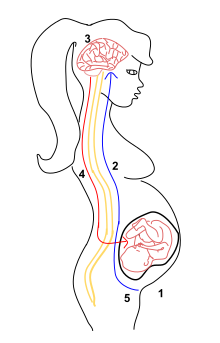
Positive feedback is the amplification of a body's response to a stimulus. For example, in childbirth, when the head of the fetus pushes up against the cervix (1) it stimulates a nerve impulse from the cervix to the brain (2). When the brain is notified, it signals the pituitary gland to release a hormone called oxytocin(3). Oxytocin is then carried via the bloodstream to the uterus (4) causing contractions, pushing the fetus towards the cervix eventually inducing childbirth.

In physiology

A number of examples of positive feedback systems may be found in physiology.

• One example is the onset of contractions in childbirth, known as the Ferguson reflex. When a contraction occurs, the hormone oxytocin causes a nerve stimulus, which stimulates the hypothalamus to produce more oxytocin, which increases uterine contractions. This results in contractions increasing in amplitude and frequency.
• Another example is the process of blood clotting. The loop is initiated when injured tissue releases signal chemicals that activate platelets in the blood. An activated platelet releases chemicals to activate more platelets, causing a rapid cascade and the formation of a blood clot.
• Lactation also involves positive feedback in that as the baby suckles on the nipple there is a nerve response into the spinal cord and up into the hypothalamus of the brain, which then stimulates the pituitary gland to produce more prolactin to produce more milk.
• A spike in estrogen during the follicular phase of the menstrual cycle causes ovulation.
• The generation of nerve signals is another example, in which the membrane of a nerve fibre causes slight leakage of sodium ions through sodium channels, resulting in a change in the membrane potential, which in turn causes more opening of channels, and so on (Hodgkin cycle). So a slight initial leakage results in an explosion of sodium leakage which creates the nerve action potential.
• In excitation–contraction coupling of the heart, an increase in intracellular calcium ions to the cardiac myocyte is detected by ryanodine receptors in the membrane of the sarcoplasmic reticulum which transport calcium out into the cytosol in a positive feedback physiological response.

In most cases, such feedback loops culminate in counter-signals being released that suppress or break the loop. Childbirth contractions stop when the baby is out of the mother's body. Chemicals break down the blood clot. Lactation stops when the baby no longer nurses.

In gene regulation

Positive feedback is a well studied phenomenon in gene regulation, where it is most often associated with bistability. Positive feedback occurs when a gene activates itself directly or indirectly via a double negative feedback loop. Genetic engineers have constructed and tested simple positive feedback networks in bacteria to demonstrate the concept of bistability. A classic example of positive feedback is the lac operon in E. coli. Positive feedback plays an integral role in cellular differentiation, development, and cancer progression, and therefore, positive feedback in gene regulation can have significant physiological consequences. Random motions in molecular dynamics coupled with positive feedback can trigger interesting effects, such as create population of phenotypically different cells from the same parent cell. This happens because noise can become amplified by positive feedback. Positive feedback can also occur in other forms of cell signaling, such as enzyme kinetics or metabolic pathways.

In evolutionary biology

Positive feedback loops have been used to describe aspects of the dynamics of change in biological evolution. For example, beginning at the macro level, Alfred J. Lotka (1945) argued that the evolution of the species was most essentially a matter of selection that fed back energy flows to capture more and more energy for use by living systems. At the human level, Richard D. Alexander (1989) proposed that social competition between and within human groups fed back to the selection of intelligence thus constantly producing more and more refined human intelligence. Crespi (2004) discussed several other examples of positive feedback loops in evolution. The analogy of Evolutionary arms races provide further examples of positive feedback in biological systems.

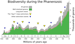
During the Phanerozoic the biodiversity shows a steady but not monotonic increase from near zero to several thousands of genera.

It has been shown that changes in biodiversity through the Phanerozoic correlate much better with hyperbolic model (widely used in demography and macrosociology) than with exponential and logistic models (traditionally used in population biology and extensively applied to fossil biodiversity as well). The latter models imply that changes in diversity are guided by a first-order positive feedback (more ancestors, more descendants) and/or a negative feedback arising from resource limitation. Hyperbolic model implies a second-order positive feedback. The hyperbolic pattern of the world population growth has been demonstrated (see below) to arise from a second-order positive feedback between the population size and the rate of technological growth. The hyperbolic character of biodiversity growth can be similarly accounted for by a positive feedback between the diversity and community structure complexity. It has been suggested that the similarity between the curves of biodiversity and human population probably comes from the fact that both are derived from the interference of the hyperbolic trend (produced by the positive feedback) with cyclical and stochastic dynamics.

Immune system

A cytokine storm, or hypercytokinemia is a potentially fatal immune reaction consisting of a positive feedback loop between cytokines and immune cells, with highly elevated levels of various cytokines. In normal immune function, positive feedback loops can be utilized to enhance the action of B lymphocytes. When a B cell binds its antibodies to an antigen and becomes activated, it begins releasing antibodies and secreting a complement protein called C3. Both C3 and a B cell's antibodies can bind to a pathogen, and when a B cell has its antibodies bind to a pathogen with C3, it speeds up that B cell's secretion of more antibodies and more C3, thus creating a positive feedback loop.

Cell death

Apoptosis is a caspase-mediated process of cellular death, whose aim is the removal of long-lived or damaged cells. A failure of this process has been implicated in prominent conditions such as cancer or Parkinson's disease. The very core of the apoptotic process is the auto-activation of caspases, which may be modeled via a positive-feedback loop. This positive feedback exerts an auto-activation of the effector caspase by means of intermediate caspases. When isolated from the rest of apoptotic pathway, this positive-feedback presents only one stable steady state, regardless of the number of intermediate activation steps of the effector caspase. When this core process is complemented with inhibitors and enhancers of caspases effects, this process presents bistability, thereby modeling the alive and dying states of a cell.

In psychology

Winner (1996) described gifted children as driven by positive feedback loops involving setting their own learning course, this feeding back satisfaction, thus further setting their learning goals to higher levels and so on. Winner termed this positive feedback loop as a "rage to master." Vandervert (2009a, 2009b) proposed that the child prodigy can be explained in terms of a positive feedback loop between the output of thinking/performing in working memory, which then is fed to the cerebellum where it is streamlined, and then fed back to working memory thus steadily increasing the quantitative and qualitative output of working memory. Vandervert also argued that this working memory/cerebellar positive feedback loop was responsible for language evolution in working memory.

In economics

Markets with social influence

Product recommendations and information about past purchases have been shown to influence consumers choices significantly whether it is for music, movie, book, technological, and other type of products. Social influence often induces a rich-get-richer phenomenon (Matthew effect) where popular products tend to become even more popular.

Market dynamics

According to the theory of reflexivity advanced by George Soros, price changes are driven by a positive feedback process whereby investors' expectations are influenced by price movements so their behaviour acts to reinforce movement in that direction until it becomes unsustainable, whereupon the feedback drives prices in the opposite direction.

Systemic risk

Systemic risk is the risk that an amplification or leverage or positive feedback process presents to a system. This is usually unknown, and under certain conditions this process can amplify exponentially and rapidly lead to destructive or chaotic behavior. A Ponzi scheme is a good example of a positive-feedback system: funds from new investors are used to pay out unusually high returns, which in turn attract more new investors, causing rapid growth toward collapse. W. Brian Arthur has also studied and written on positive feedback in the economy (e.g. W. Brian Arthur, 1990). Hyman Minsky proposed a theory that certain credit expansion practices could make a market economy into "a deviation amplifying system" that could suddenly collapse, sometimes called a "Minsky moment".

Simple systems that clearly separate the inputs from the outputs are not prone to systemic risk. This risk is more likely as the complexity of the system increases, because it becomes more difficult to see or analyze all the possible combinations of variables in the system even under careful stress testing conditions. The more efficient a complex system is, the more likely it is to be prone to systemic risks, because it takes only a small amount of deviation to disrupt the system. Therefore, well-designed complex systems generally have built-in features to avoid this condition, such as a small amount of friction, or resistance, or inertia, or time delay to decouple the outputs from the inputs within the system. These factors amount to an inefficiency, but they are necessary to avoid instabilities.

The 2010 Flash Crash incident was blamed on the practice of high-frequency trading (HFT), although whether HFT really increases systemic risk remains controversial.

Human population growth

Agriculture and human population can be considered to be in a positive feedback mode, which means that one drives the other with increasing intensity. It is suggested that this positive feedback system will end sometime with a catastrophe, as modern agriculture is using up all of the easily available phosphate and is resorting to highly efficient monocultures which are more susceptible to systemic risk.

Technological innovation and human population can be similarly considered, and this has been offered as an explanation for the apparent hyperbolic growth of the human population in the past, instead of a simpler exponential growth. It is proposed that the growth rate is accelerating because of second-order positive feedback between population and technology. Technological growth increases the carrying capacity of land for people, which leads to a growing population, and this in turn drives further technological growth.

Prejudice, social institutions and poverty

Gunnar Myrdal described a vicious circle of increasing inequalities, and poverty, which is known as "circular cumulative causation".

In meteorology

Drought intensifies through positive feedback. A lack of rain decreases soil moisture, which kills plants and/or causes them to release less water through transpiration. Both factors limit evapotranspiration, the process by which water vapor is added to the atmosphere from the surface, and add dry dust to the atmosphere, which absorbs water. Less water vapor means both low dew point temperatures and more efficient daytime heating, decreasing the chances of humidity in the atmosphere leading to cloud formation. Lastly, without clouds, there cannot be rain, and the loop is complete.

In climatology

Climate "forcings" may push a climate system in the direction of warming or cooling, for example, increased atmospheric concentrations of greenhouse gases cause warming at the surface. Forcings are external to the climate system and feedbacks are internal processes of the system. Some feedback mechanisms act in relative isolation to the rest of the climate system while others are tightly coupled. Forcings, feedbacks and the dynamics of the climate system determine how much and how fast the climate changes. The main positive feedback in global warming is the tendency of warming to increase the amount of water vapor in the atmosphere, which in turn leads to further warming. The main negative feedback comes from the Stefan–Boltzmann law, the amount of heat radiated from the Earth into space is proportional to the fourth power of the temperature of Earth's surface and atmosphere.

Other examples of positive feedback subsystems in climatology include:

• A warmer atmosphere will melt ice and this changes the albedo which further warms the atmosphere.
• Methane hydrates can be unstable so that a warming ocean could release more methane, which is also a greenhouse gas.
• Peat, occurring naturally in peat bogs, contains carbon. When peat dries it decomposes, and may additionally burn. Peat also releases nitrous oxide.
• Global warming affects the cloud distribution. Clouds at higher altitudes enhance the greenhouse effects, while low clouds mainly reflect back sunlight, having opposite effects on temperature.

The Intergovernmental Panel on Climate Change (IPCC) Fourth Assessment Report states that "Anthropogenic warming could lead to some effects that are abrupt or irreversible, depending upon the rate and magnitude of the climate change."

In sociology

A self-fulfilling prophecy is a social positive feedback loop between beliefs and behavior: if enough people believe that something is true, their behavior can make it true, and observations of their behavior may in turn increase belief. A classic example is a bank run.

Another sociological example of positive feedback is the network effect. When more people are encouraged to join a network this increases the reach of the network therefore the network expands ever more quickly. A viral video is an example of the network effect in which links to a popular video are shared and redistributed, ensuring that more people see the video and then re-publish the links. This is the basis for many social phenomena, including Ponzi schemes and chain letters. In many cases population size is the limiting factor to the feedback effect.

In chemistry

If a chemical reaction causes the release of heat, and the reaction itself happens faster at higher temperatures, then there is a high likelihood of positive feedback. If the heat produced is not removed from the reactants fast enough, thermal runaway can occur and very quickly lead to a chemical explosion.

In conservation

Many wildlife are hunted for their parts which can be quite valuable. The closer to extinction that targeted species become, the higher the price there is on their parts. This is an example of positive feedback

Matthew effect

From Wikipedia, the free encyclopedia

Jump to navigation Jump to search

The Matthew effect of accumulated advantage, Matthew principle, or Matthew effect for short, is sometimes summarized by the adage "the rich get richer and the poor get poorer". The concept is applicable to matters of fame or status, but may also be applied literally to cumulative advantage of economic capital. In the beginning, Matthew effects were primarily focused on the inequality in the way scientists were recognized for their work. However, Norman Storer, of Columbia University, led a new wave of research. He believed he discovered that the inequality that existed in the social sciences also existed in other institutions.

The term was coined by sociologist Robert K. Merton in 1968 and takes its name from the parable of the talents or minas in the biblical Gospel of Matthew. Merton credited his collaborator and wife, sociologist Harriet Zuckerman, as co-author of the concept of the Matthew effect.

Etymology

The concept is named according to two of the parables of Jesus in the synoptic Gospels (Table 2, of the Eusebian Canons).

The concept concludes both synoptic versions of the parable of the talents:

For to every one who has will more be given, and he will have abundance; but from him who has not, even what he has will be taken away.

— Matthew 25:29, RSV.

I tell you, that to every one who has will more be given; but from him who has not, even what he has will be taken away.

— Luke 19:26, RSV.

The concept concludes two of the three synoptic versions of the parable of the lamp under a bushel (absent in the version of Matthew):

For to him who has will more be given; and from him who has not, even what he has will be taken away

— Mark 4:25, RSV.

Take heed then how you hear; for to him who has will more be given, and from him who has not, even what he thinks that he has will be taken away.

— Luke 8:18, RSV.

The concept is presented again in Matthew outside of a parable during Christ's explanation to his disciples of the purpose of parables:

And he answered them, "To you it has been given to know the secrets of the kingdom of heaven, but to them it has not been given. For to him who has will more be given, and he will have abundance; but from him who has not, even what he has will be taken away."

— Matthew 13:11–12, RSV.

Sociology of science

In the sociology of science, "Matthew effect" was a term coined by Robert K. Merton to describe how, among other things, eminent scientists will often get more credit than a comparatively unknown researcher, even if their work is similar; it also means that credit will usually be given to researchers who are already famous. For example, a prize will almost always be awarded to the most senior researcher involved in a project, even if all the work was done by a graduate student. This was later formulated by Stephen Stigler as Stigler's law of eponymy – "No scientific discovery is named after its original discoverer" – with Stigler explicitly naming Merton as the true discoverer, making his "law" an example of itself.

Merton furthermore argued that in the scientific community the Matthew effect reaches beyond simple reputation to influence the wider communication system, playing a part in social selection processes and resulting in a concentration of resources and talent. He gave as an example the disproportionate visibility given to articles from acknowledged authors, at the expense of equally valid or superior articles written by unknown authors. He also noted that the concentration of attention on eminent individuals can lead to an increase in their self-assurance, pushing them to perform research in important but risky problem areas.

Examples

As credit is valued in science, specific claims of the Matthew effect are contentious. Many examples below exemplify more famous scientists getting credit for discoveries due to their fame, even as other less notable scientists had preempted their work.

• Experiments manipulating download counts or bestseller lists for books and music have shown consumer activity follows the apparent popularity.
• In algorithmic information theory, the notion of Kolmogorov complexity is named after the famous mathematician Andrey Kolmogorov even though it was independently discovered and published by Ray Solomonoff a year before Kolmogorov. Li and Vitanyi, in "An Introduction to Kolmogorov Complexity and Its Applications" (p. 84), write:

Ray Solomonoff ... introduced [what is now known as] "Kolmogorov complexity" in a long journal paper in 1964. ... This makes Solomonoff the first inventor and raises the question whether we should talk about Solomonoff complexity. ...

• There are many uncontroversial examples of the Matthew effect in mathematics, where a concept is due to one mathematician (and well-documented as such), but is attributed to a later (possibly much later), more famous mathematician who worked on it. For instance, the Poincaré disk model and Poincaré half-plane model of hyperbolic space are both named for Henri Poincaré, but were introduced by Eugenio Beltrami in 1868 (when Poincaré was 14 and had not as yet contributed to hyperbolic geometry).
• A model for career progress quantitatively incorporates the Matthew Effect in order to predict the distribution of individual career length in competitive professions. The model predictions are validated by analyzing the empirical distributions of career length for careers in science and professional sports (e.g. Major League Baseball). As a result, the disparity between the large number of short careers and the relatively small number of extremely long careers can be explained by the "rich-get-richer" mechanism, which in this framework, provides more experienced and more reputable individuals with a competitive advantage in obtaining new career opportunities.
• In his 2011 book The Better Angels of Our Nature: Why Violence Has Declined, cognitive psychologist Steven Pinker refers to the Matthew Effect in societies, whereby everything seems to go right in some, and wrong in others. He speculates in Chapter 9 that this could be the result of a positive feedback loop in which reckless behavior by some individuals creates a chaotic environment that encourages reckless behavior by others. He cites research by Martin Daly and Margo Wilson showing that the more unstable the environment, the more steeply people discount the future, and thus the less forward-looking their behavior.
• A large Matthew effect was discovered in a study of science funding in the Netherlands, where winners just above the funding threshold were found to accumulate more than twice as much funding during the subsequent eight years as non-winners with near-identical review scores that fell just below the threshold.

In science, dramatic differences in the productivity may be explained by three phenomena: sacred spark, cumulative advantage, and search costs minimization by journal editors. The sacred spark paradigm suggests that scientists differ in their initial abilities, talent, skills, persistence, work habits, etc. that provide particular individuals with an early advantage. These factors have a multiplicative effect which helps these scholars succeed later. The cumulative advantage model argues that an initial success helps a researcher gain access to resources (e.g., teaching release, best graduate students, funding, facilities, etc.), which in turn results in further success. Search costs minimization by journal editors takes place when editors try to save time and effort by consciously or subconsciously selecting articles from well-known scholars. Whereas the exact mechanism underlying these phenomena is yet unknown, it is documented that a minority of all academics produce the most research output and attract the most citations.

Education

In education, the term "Matthew effect" has been adopted by psychologist Keith Stanovich to describe a phenomenon observed in research on how new readers acquire the skills to read: early success in acquiring reading skills usually leads to later successes in reading as the learner grows, while failing to learn to read before the third or fourth year of schooling may be indicative of lifelong problems in learning new skills.

This is because children who fall behind in reading would read less, increasing the gap between them and their peers. Later, when students need to "read to learn" (where before they were learning to read), their reading difficulty creates difficulty in most other subjects. In this way they fall further and further behind in school, dropping out at a much higher rate than their peers.

In the words of Stanovich:

Slow reading acquisition has cognitive, behavioral, and motivational consequences that slow the development of other cognitive skills and inhibit performance on many academic tasks. In short, as reading develops, other cognitive processes linked to it track the level of reading skill. Knowledge bases that are in reciprocal relationships with reading are also inhibited from further development. The longer this developmental sequence is allowed to continue, the more generalized the deficits will become, seeping into more and more areas of cognition and behavior. Or to put it more simply – and sadly – in the words of a tearful nine-year-old, already falling frustratingly behind his peers in reading progress, "Reading affects everything you do."

The Matthew effect plays a role in today's educational system.

Students around the United States participate in the SAT every year to then send those scores to the colleges to which they are applying. The distributor of the SAT, the College board, conducted a study based on the income earned by the families of the test takers. The results showed the Matthew effect is prevalent when it comes to a family's economic earnings: "Students from families earning more than $200,000 a year average a combined score of 1,714, while students from families earning under $20,000 a year average a combined score of 1,326."

Not only do students with a wealthier family score better, but statistics show that students with parents that have accomplished more in school perform better as well. A student with a parent with a graduate degree, for example, averages 300 points higher on their SAT compared to a student with a parent with only a high school degree.

Network science

In network science, the Matthew effect is used to describe the preferential attachment of earlier nodes in a network, which explains that these nodes tend to attract more links early on. "Because of preferential attachment, a node that acquires more connections than another one will increase its connectivity at a higher rate, and thus an initial difference in the connectivity between two nodes will increase further as the network grows, while the degree of individual nodes will grow proportional with the square root of time." The Matthew Effect therefore explains the growth of some nodes in vast networks such as the Internet.

Markets with social influence

Social influence often induces a rich-get-richer phenomenon where popular products tend to become even more popular. An example of the Matthew Effect's role on social influence. Salganik, Dodds, and Watts created an experimental virtual market named MUSICLAB. In MUSICLAB, people could listen to music and choose to download the songs they enjoyed the most. The song choices were unknown songs produced by unknown bands. There were two groups tested; one group was given zero additional information on the songs and one group was told the popularity of each song and the number of times it had previously been downloaded. As a result, the group that saw which songs were the most popular and were downloaded the most were then biased to choose those songs as well. The songs that were most popular and downloaded the most stayed at the top of the list and consistently received the most plays. To summarize the experiments findings, the performance rankings had the largest effect boosting expected downloads the most. Download rankings had a decent effect; however, not as impactful as the performance rankings. Also, Abeliuk et al. (2016) proved that when utilizing “performance rankings”, a monopoly will be created for the most popular songs.

Political science

Liberalization in autocracies is more likely to succeed in countries with the advantage of a better starting point concerning political institutions, GDP, and education. These more privileged countries can also carry out key reforms more rapidly, and are able to do so even in areas with no initial advantage.

Power law

From Wikipedia, the free encyclopedia

https://en.wikipedia.org/wiki/Power_law 

 

An example power-law graph that demonstrates ranking of popularity. To the right is the long tail, and to the left are the few that dominate (also known as the 80–20 rule).

In statistics, a power law is a functional relationship between two quantities, where a relative change in one quantity results in a proportional relative change in the other quantity, independent of the initial size of those quantities: one quantity varies as a power of another. For instance, considering the area of a square in terms of the length of its side, if the length is doubled, the area is multiplied by a factor of four.

Empirical examples

The distributions of a wide variety of physical, biological, and man-made phenomena approximately follow a power law over a wide range of magnitudes: these include the sizes of craters on the moon and of solar flares, the foraging pattern of various species, the sizes of activity patterns of neuronal populations, the frequencies of words in most languages, frequencies of family names, the species richness in clades of organisms, the sizes of power outages, criminal charges per convict, volcanic eruptions, human judgements of stimulus intensity and many other quantities. Few empirical distributions fit a power law for all their values, but rather follow a power law in the tail. Acoustic attenuation follows frequency power-laws within wide frequency bands for many complex media. Allometric scaling laws for relationships between biological variables are among the best known power-law functions in nature.

Properties

Scale invariance

One attribute of power laws is their scale invariance. Given a relation ${\displaystyle f(x)=ax^{-k}}$, scaling the argument ${\displaystyle x}$ by a constant factor ${\displaystyle c}$ causes only a proportionate scaling of the function itself. That is,

${\displaystyle f(cx)=a(cx)^{-k}=c^{-k}f(x)\propto f(x),\!}$

where ${\displaystyle \propto }$ denotes direct proportionality. That is, scaling by a constant ${\displaystyle c}$ simply multiplies the original power-law relation by the constant ${\displaystyle c^{-k}}$. Thus, it follows that all power laws with a particular scaling exponent are equivalent up to constant factors, since each is simply a scaled version of the others. This behavior is what produces the linear relationship when logarithms are taken of both ${\displaystyle f(x)}$ and ${\displaystyle x}$, and the straight-line on the log–log plot is often called the signature of a power law. With real data, such straightness is a necessary, but not sufficient, condition for the data following a power-law relation. In fact, there are many ways to generate finite amounts of data that mimic this signature behavior, but, in their asymptotic limit, are not true power laws (e.g., if the generating process of some data follows a Log-normal distribution). Thus, accurately fitting and validating power-law models is an active area of research in statistics; see below.

Lack of well-defined average value

A power-law ${\displaystyle x^{-k}}$ has a well-defined mean over ${\displaystyle x\in [1,\infty )}$ only if ${\displaystyle k>2}$, and it has a finite variance only if ${\displaystyle k>3}$; most identified power laws in nature have exponents such that the mean is well-defined but the variance is not, implying they are capable of black swan behavior. This can be seen in the following thought experiment: imagine a room with your friends and estimate the average monthly income in the room. Now imagine the world's richest person entering the room, with a monthly income of about 1 billion US$. What happens to the average income in the room? Income is distributed according to a power-law known as the Pareto distribution (for example, the net worth of Americans is distributed according to a power law with an exponent of 2).

On the one hand, this makes it incorrect to apply traditional statistics that are based on variance and standard deviation (such as regression analysis). On the other hand, this also allows for cost-efficient interventions. For example, given that car exhaust is distributed according to a power-law among cars (very few cars contribute to most contamination) it would be sufficient to eliminate those very few cars from the road to reduce total exhaust substantially.

The median does exist, however: for a power law x ^–k, with exponent ${\displaystyle k>1}$, it takes the value 2^{1/(k – 1)}x_min, where x_min is the minimum value for which the power law holds.

Universality

The equivalence of power laws with a particular scaling exponent can have a deeper origin in the dynamical processes that generate the power-law relation. In physics, for example, phase transitions in thermodynamic systems are associated with the emergence of power-law distributions of certain quantities, whose exponents are referred to as the critical exponents of the system. Diverse systems with the same critical exponents—that is, which display identical scaling behaviour as they approach criticality—can be shown, via renormalization group theory, to share the same fundamental dynamics. For instance, the behavior of water and CO₂ at their boiling points fall in the same universality class because they have identical critical exponents. In fact, almost all material phase transitions are described by a small set of universality classes. Similar observations have been made, though not as comprehensively, for various self-organized critical systems, where the critical point of the system is an attractor. Formally, this sharing of dynamics is referred to as universality, and systems with precisely the same critical exponents are said to belong to the same universality class.

Power-law functions

Scientific interest in power-law relations stems partly from the ease with which certain general classes of mechanisms generate them. The demonstration of a power-law relation in some data can point to specific kinds of mechanisms that might underlie the natural phenomenon in question, and can indicate a deep connection with other, seemingly unrelated systems; see also universality above. The ubiquity of power-law relations in physics is partly due to dimensional constraints, while in complex systems, power laws are often thought to be signatures of hierarchy or of specific stochastic processes. A few notable examples of power laws are Pareto's law of income distribution, structural self-similarity of fractals, and scaling laws in biological systems. Research on the origins of power-law relations, and efforts to observe and validate them in the real world, is an active topic of research in many fields of science, including physics, computer science, linguistics, geophysics, neuroscience, sociology, economics and more.

However, much of the recent interest in power laws comes from the study of probability distributions: The distributions of a wide variety of quantities seem to follow the power-law form, at least in their upper tail (large events). The behavior of these large events connects these quantities to the study of theory of large deviations (also called extreme value theory), which considers the frequency of extremely rare events like stock market crashes and large natural disasters. It is primarily in the study of statistical distributions that the name "power law" is used.

In empirical contexts, an approximation to a power-law ${\displaystyle o(x^{k})}$ often includes a deviation term ${\displaystyle \varepsilon }$, which can represent uncertainty in the observed values (perhaps measurement or sampling errors) or provide a simple way for observations to deviate from the power-law function (perhaps for stochastic reasons):

${\displaystyle y=ax^{k}+\varepsilon .\!}$

Mathematically, a strict power law cannot be a probability distribution, but a distribution that is a truncated power function is possible: ${\displaystyle p(x)=Cx^{-\alpha }}$ for ${\displaystyle x>x_{\text{min}}}$ where the exponent ${\displaystyle \alpha }$ (Greek letter alpha, not to be confused with scaling factor ${\displaystyle a}$ used above) is greater than 1 (otherwise the tail has infinite area), the minimum value ${\displaystyle x_{\text{min}}}$ is needed otherwise the distribution has infinite area as x approaches 0, and the constant C is a scaling factor to ensure that the total area is 1, as required by a probability distribution. More often one uses an asymptotic power law – one that is only true in the limit; see power-law probability distributions below for details. Typically the exponent falls in the range ${\displaystyle 2<\alpha <3}$, though not always.

Examples

More than a hundred power-law distributions have been identified in physics (e.g. sandpile avalanches), biology (e.g. species extinction and body mass), and the social sciences (e.g. city sizes and income). Among them are:

Astronomy

• Kepler's third law
• The initial mass function of stars
• The differential energy spectrum of cosmic-ray nuclei
• The M-sigma relation

Criminology

• number of charges per criminal offender

Physics

• The Angstrom exponent in aerosol optics
• The frequency-dependency of acoustic attenuation in complex media
• Stevens's power law of psychophysics
• The Stefan–Boltzmann law
• The input-voltage–output-current curves of field-effect transistors and vacuum tubes approximate a square-law relationship, a factor in "tube sound".
• Square-cube law (ratio of surface area to volume)
• A 3/2-power law can be found in the plate characteristic curves of triodes.
• The inverse-square laws of Newtonian gravity and electrostatics, as evidenced by the gravitational potential and Electrostatic potential, respectively.
• Self-organized criticality with a critical point as an attractor
• Model of van der Waals force
• Force and potential in simple harmonic motion
• Gamma correction relating light intensity with voltage
• Behaviour near second-order phase transitions involving critical exponents
• The safe operating area relating to maximum simultaneous current and voltage in power semiconductors.
• Supercritical state of matter and supercritical fluids, such as supercritical exponents of heat capacity and viscosity.
• The Curie-von Schweidler law in dielectric responses to step DC voltage input.
• The damping force over speed relation in antiseismic dampers calculus

Biology

• Kleiber's law relating animal metabolism to size, and allometric laws in general
• The two-thirds power law, relating speed to curvature in the human motor system
• The Taylor's law relating mean population size and variance of populations sizes in ecology
• Neuronal avalanches
• The species richness (number of species) in clades of freshwater fishes
• The Harlow Knapp effect, where a subset of the kinases found in the human body compose a majority of published research

Meteorology

• The size of rain-shower cells, energy dissipation in cyclones, and the diameters of dust devils on Earth and Mars 

General science

• Exponential growth and random observation (or killing)
• Progress through exponential growth and exponential diffusion of innovations
• Highly optimized tolerance
• Proposed form of experience curve effects
• Pink noise
• The law of stream numbers, and the law of stream lengths (Horton's laws describing river systems)
• Populations of cities (Gibrat's law)
• Bibliograms, and frequencies of words in a text (Zipf's law)
• 90–9–1 principle on wikis (also referred to as the 1% rule)
• Richardson's Law for the severity of violent conflicts (wars and terrorism)
• The relationship between a CPU's cache size and the number of cache misses follows the power law of cache misses.
• The spectral density of the weight matrices of deep neural networks

Mathematics

• Fractals
• Pareto distribution and the Pareto principle also called the "80–20 rule"
• Zipf's law in corpus analysis and population distributions amongst others, where frequency of an item or event is inversely proportional to its frequency rank (i.e. the second most frequent item/event occurs half as often as the most frequent item, the third most frequent item/event occurs one third as often as the most frequent item, and so on).
• Zeta distribution (discrete)
• Yule–Simon distribution (discrete)
• Student's t-distribution (continuous), of which the Cauchy distribution is a special case
• Lotka's law
• The scale-free network model

Economics

• Population sizes of cities in a region or urban network, Zipf's law.

• Distribution of artists by the average price of their artworks.

• Distribution of income in a market economy.

• Distribution of degrees in banking networks.

Finance

• The mean absolute change of the logarithmic mid-prices
• Number of tick counts over time
• Size of the maximum price move
• Average waiting time of a directional change
• Average waiting time of an overshoot

Variants

Broken power law

Some models of the initial mass function use a broken power law; here Kroupa (2001) in red.

A broken power law is a piecewise function, consisting of two or more power laws, combined with a threshold. For example, with two power laws:

${\displaystyle f(x)\propto x^{\alpha _{1}}}$ for ${\displaystyle x<x_{\text{th}},}$

${\displaystyle f(x)\propto x_{\text{th}}^{\alpha _{1}-\alpha _{2}}x^{\alpha _{2}}{\text{ for }}x>x_{\text{th}}}$.

Power law with exponential cutoff

A power law with an exponential cutoff is simply a power law multiplied by an exponential function:

${\displaystyle f(x)\propto x^{\alpha }e^{\beta x}.}$

Curved power law

${\displaystyle f(x)\propto x^{\alpha +\beta x}}$

Power-law probability distributions

In a looser sense, a power-law probability distribution is a distribution whose density function (or mass function in the discrete case) has the form, for large values of ${\displaystyle x}$,

${\displaystyle P(X>x)\sim L(x)x^{-(\alpha -1)}}$

where ${\displaystyle \alpha >1}$, and ${\displaystyle L(x)}$ is a slowly varying function, which is any function that satisfies ${\displaystyle \lim _{x\rightarrow \infty }L(r\,x)/L(x)=1}$ for any positive factor ${\displaystyle r}$. This property of ${\displaystyle L(x)}$ follows directly from the requirement that ${\displaystyle p(x)}$ be asymptotically scale invariant; thus, the form of ${\displaystyle L(x)}$ only controls the shape and finite extent of the lower tail. For instance, if ${\displaystyle L(x)}$ is the constant function, then we have a power law that holds for all values of ${\displaystyle x}$. In many cases, it is convenient to assume a lower bound ${\displaystyle x_{\mathrm {min} }}$ from which the law holds. Combining these two cases, and where ${\displaystyle x}$ is a continuous variable, the power law has the form

${\displaystyle p(x)={\frac {\alpha -1}{x_{\min }}}\left({\frac {x}{x_{\min }}}\right)^{-\alpha },}$

where the pre-factor to ${\displaystyle {\frac {\alpha -1}{x_{\min }}}}$ is the normalizing constant. We can now consider several properties of this distribution. For instance, its moments are given by

${\displaystyle \langle x^{m}\rangle =\int _{x_{\min }}^{\infty }x^{m}p(x)\,\mathrm {d} x={\frac {\alpha -1}{\alpha -1-m}}x_{\min }^{m}}$

which is only well defined for ${\displaystyle m<\alpha -1}$. That is, all moments ${\displaystyle m\geq \alpha -1}$ diverge: when ${\displaystyle \alpha \leq 2}$, the average and all higher-order moments are infinite; when ${\displaystyle 2<\alpha <3}$, the mean exists, but the variance and higher-order moments are infinite, etc. For finite-size samples drawn from such distribution, this behavior implies that the central moment estimators (like the mean and the variance) for diverging moments will never converge – as more data is accumulated, they continue to grow. These power-law probability distributions are also called Pareto-type distributions, distributions with Pareto tails, or distributions with regularly varying tails.

A modification, which does not satisfy the general form above, with an exponential cutoff, is

${\displaystyle p(x)\propto L(x)x^{-\alpha }\mathrm {e} ^{-\lambda x}.}$

In this distribution, the exponential decay term ${\displaystyle \mathrm {e} ^{-\lambda x}}$ eventually overwhelms the power-law behavior at very large values of ${\displaystyle x}$. This distribution does not scale and is thus not asymptotically as a power law; however, it does approximately scale over a finite region before the cutoff. The pure form above is a subset of this family, with ${\displaystyle \lambda =0}$. This distribution is a common alternative to the asymptotic power-law distribution because it naturally captures finite-size effects.

The Tweedie distributions are a family of statistical models characterized by closure under additive and reproductive convolution as well as under scale transformation. Consequently, these models all express a power-law relationship between the variance and the mean. These models have a fundamental role as foci of mathematical convergence similar to the role that the normal distribution has as a focus in the central limit theorem. This convergence effect explains why the variance-to-mean power law manifests so widely in natural processes, as with Taylor's law in ecology and with fluctuation scaling in physics. It can also be shown that this variance-to-mean power law, when demonstrated by the method of expanding bins, implies the presence of 1/f noise and that 1/f noise can arise as a consequence of this Tweedie convergence effect.

Graphical methods for identification

Although more sophisticated and robust methods have been proposed, the most frequently used graphical methods of identifying power-law probability distributions using random samples are Pareto quantile-quantile plots (or Pareto Q–Q plots), mean residual life plots and log–log plots. Another, more robust graphical method uses bundles of residual quantile functions. (Please keep in mind that power-law distributions are also called Pareto-type distributions.) It is assumed here that a random sample is obtained from a probability distribution, and that we want to know if the tail of the distribution follows a power law (in other words, we want to know if the distribution has a "Pareto tail"). Here, the random sample is called "the data".

Pareto Q–Q plots compare the quantiles of the log-transformed data to the corresponding quantiles of an exponential distribution with mean 1 (or to the quantiles of a standard Pareto distribution) by plotting the former versus the latter. If the resultant scatterplot suggests that the plotted points " asymptotically converge" to a straight line, then a power-law distribution should be suspected. A limitation of Pareto Q–Q plots is that they behave poorly when the tail index ${\displaystyle \alpha }$ (also called Pareto index) is close to 0, because Pareto Q–Q plots are not designed to identify distributions with slowly varying tails.

On the other hand, in its version for identifying power-law probability distributions, the mean residual life plot consists of first log-transforming the data, and then plotting the average of those log-transformed data that are higher than the i-th order statistic versus the i-th order statistic, for i = 1, ..., n, where n is the size of the random sample. If the resultant scatterplot suggests that the plotted points tend to "stabilize" about a horizontal straight line, then a power-law distribution should be suspected. Since the mean residual life plot is very sensitive to outliers (it is not robust), it usually produces plots that are difficult to interpret; for this reason, such plots are usually called Hill horror plots 

A straight line on a log–log plot is necessary but insufficient evidence for power-laws, the slope of the straight line corresponds to the power law exponent.

Log–log plots are an alternative way of graphically examining the tail of a distribution using a random sample. Caution has to be exercised however as a log–log plot is necessary but insufficient evidence for a power law relationship, as many non power-law distributions will appear as straight lines on a log–log plot. This method consists of plotting the logarithm of an estimator of the probability that a particular number of the distribution occurs versus the logarithm of that particular number. Usually, this estimator is the proportion of times that the number occurs in the data set. If the points in the plot tend to "converge" to a straight line for large numbers in the x axis, then the researcher concludes that the distribution has a power-law tail. Examples of the application of these types of plot have been published. A disadvantage of these plots is that, in order for them to provide reliable results, they require huge amounts of data. In addition, they are appropriate only for discrete (or grouped) data.

Another graphical method for the identification of power-law probability distributions using random samples has been proposed. This methodology consists of plotting a bundle for the log-transformed sample. Originally proposed as a tool to explore the existence of moments and the moment generation function using random samples, the bundle methodology is based on residual quantile functions (RQFs), also called residual percentile functions, which provide a full characterization of the tail behavior of many well-known probability distributions, including power-law distributions, distributions with other types of heavy tails, and even non-heavy-tailed distributions. Bundle plots do not have the disadvantages of Pareto Q–Q plots, mean residual life plots and log–log plots mentioned above (they are robust to outliers, allow visually identifying power laws with small values of ${\displaystyle \alpha }$, and do not demand the collection of much data). In addition, other types of tail behavior can be identified using bundle plots.

Plotting power-law distributions

In general, power-law distributions are plotted on doubly logarithmic axes, which emphasizes the upper tail region. The most convenient way to do this is via the (complementary) cumulative distribution (cdf), ${\displaystyle P(x)=\mathrm {Pr} (X>x)}$,

${\displaystyle P(x)=\Pr(X>x)=C\int _{x}^{\infty }p(X)\,\mathrm {d} X={\frac {\alpha -1}{x_{\min }^{-\alpha +1}}}\int _{x}^{\infty }X^{-\alpha }\,\mathrm {d} X=\left({\frac {x}{x_{\min }}}\right)^{-\alpha +1}.}$

The cdf is also a power-law function, but with a smaller scaling exponent. For data, an equivalent form of the cdf is the rank-frequency approach, in which we first sort the ${\displaystyle n}$ observed values in ascending order, and plot them against the vector ${\displaystyle \left[1,{\frac {n-1}{n}},{\frac {n-2}{n}},\dots ,{\frac {1}{n}}\right]}$.

Although it can be convenient to log-bin the data, or otherwise smooth the probability density (mass) function directly, these methods introduce an implicit bias in the representation of the data, and thus should be avoided. The cdf, on the other hand, is more robust to (but not without) such biases in the data and preserves the linear signature on doubly logarithmic axes. Though a cdf representation is favored over that of the pdf while fitting a power law to the data with the linear least square method, it is not devoid of mathematical inaccuracy. Thus, while estimating exponents of a power law distribution, maximum likelihood estimator is recommended.

Estimating the exponent from empirical data

There are many ways of estimating the value of the scaling exponent for a power-law tail, however not all of them yield unbiased and consistent answers. Some of the most reliable techniques are often based on the method of maximum likelihood. Alternative methods are often based on making a linear regression on either the log–log probability, the log–log cumulative distribution function, or on log-binned data, but these approaches should be avoided as they can all lead to highly biased estimates of the scaling exponent.

Maximum likelihood

For real-valued, independent and identically distributed data, we fit a power-law distribution of the form

${\displaystyle p(x)={\frac {\alpha -1}{x_{\min }}}\left({\frac {x}{x_{\min }}}\right)^{-\alpha }}$

to the data ${\displaystyle x\geq x_{\min }}$, where the coefficient ${\displaystyle {\frac {\alpha -1}{x_{\min }}}}$ is included to ensure that the distribution is normalized. Given a choice for ${\displaystyle x_{\min }}$, the log likelihood function becomes:

${\displaystyle {\mathcal {L}}(\alpha )=\log \prod _{i=1}^{n}{\frac {\alpha -1}{x_{\min }}}\left({\frac {x_{i}}{x_{\min }}}\right)^{-\alpha }}$

The maximum of this likelihood is found by differentiating with respect to parameter ${\displaystyle \alpha }$, setting the result equal to zero. Upon rearrangement, this yields the estimator equation:

${\displaystyle {\hat {\alpha }}=1+n\left[\sum _{i=1}^{n}\ln {\frac {x_{i}}{x_{\min }}}\right]^{-1}}$

where ${\displaystyle \{x_{i}\}}$ are the ${\displaystyle n}$ data points ${\displaystyle x_{i}\geq x_{\min }}$. This estimator exhibits a small finite sample-size bias of order ${\displaystyle O(n^{-1})}$, which is small when n > 100. Further, the standard error of the estimate is ${\displaystyle \sigma ={\frac {{\hat {\alpha }}-1}{\sqrt {n}}}+O(n^{-1})}$. This estimator is equivalent to the popular Hill estimator from quantitative finance and extreme value theory.

For a set of n integer-valued data points ${\displaystyle \{x_{i}\}}$, again where each ${\displaystyle x_{i}\geq x_{\min }}$, the maximum likelihood exponent is the solution to the transcendental equation

${\displaystyle {\frac {\zeta '({\hat {\alpha }},x_{\min })}{\zeta ({\hat {\alpha }},x_{\min })}}=-{\frac {1}{n}}\sum _{i=1}^{n}\ln {\frac {x_{i}}{x_{\min }}}}$

where ${\displaystyle \zeta (\alpha ,x_{\mathrm {min} })}$ is the incomplete zeta function. The uncertainty in this estimate follows the same formula as for the continuous equation. However, the two equations for ${\displaystyle {\hat {\alpha }}}$ are not equivalent, and the continuous version should not be applied to discrete data, nor vice versa.

Further, both of these estimators require the choice of ${\displaystyle x_{\min }}$. For functions with a non-trivial ${\displaystyle L(x)}$ function, choosing ${\displaystyle x_{\min }}$ too small produces a significant bias in ${\displaystyle {\hat {\alpha }}}$, while choosing it too large increases the uncertainty in ${\displaystyle {\hat {\alpha }}}$, and reduces the statistical power of our model. In general, the best choice of ${\displaystyle x_{\min }}$ depends strongly on the particular form of the lower tail, represented by ${\displaystyle L(x)}$ above.

More about these methods, and the conditions under which they can be used, can be found in . Further, this comprehensive review article provides usable code (Matlab, Python, R and C++) for estimation and testing routines for power-law distributions.

Kolmogorov–Smirnov estimation

Another method for the estimation of the power-law exponent, which does not assume independent and identically distributed (iid) data, uses the minimization of the Kolmogorov–Smirnov statistic, ${\displaystyle D}$, between the cumulative distribution functions of the data and the power law:

${\displaystyle {\hat {\alpha }}={\underset {\alpha }{\operatorname {arg\,min} }}\,D_{\alpha }}$

with

${\displaystyle D_{\alpha }=\max _{x}|P_{\mathrm {emp} }(x)-P_{\alpha }(x)|}$

where ${\displaystyle P_{\mathrm {emp} }(x)}$ and ${\displaystyle P_{\alpha }(x)}$ denote the cdfs of the data and the power law with exponent ${\displaystyle \alpha }$, respectively. As this method does not assume iid data, it provides an alternative way to determine the power-law exponent for data sets in which the temporal correlation can not be ignored.

Two-point fitting method

This criterion can be applied for the estimation of power-law exponent in the case of scale free distributions and provides a more convergent estimate than the maximum likelihood method. It has been applied to study probability distributions of fracture apertures. In some contexts the probability distribution is described, not by the cumulative distribution function, by the cumulative frequency of a property X, defined as the number of elements per meter (or area unit, second etc.) for which X > x applies, where x is a variable real number. As an example, the cumulative distribution of the fracture aperture, X, for a sample of N elements is defined as 'the number of fractures per meter having aperture greater than x . Use of cumulative frequency has some advantages, e.g. it allows one to put on the same diagram data gathered from sample lines of different lengths at different scales (e.g. from outcrop and from microscope).

Validating power laws

Although power-law relations are attractive for many theoretical reasons, demonstrating that data does indeed follow a power-law relation requires more than simply fitting a particular model to the data. This is important for understanding the mechanism that gives rise to the distribution: superficially similar distributions may arise for significantly different reasons, and different models yield different predictions, such as extrapolation.

For example, log-normal distributions are often mistaken for power-law distributions: a data set drawn from a lognormal distribution will be approximately linear for large values (corresponding to the upper tail of the lognormal being close to a power law), but for small values the lognormal will drop off significantly (bowing down), corresponding to the lower tail of the lognormal being small (there are very few small values, rather than many small values in a power law).

For example, Gibrat's law about proportional growth processes produce distributions that are lognormal, although their log–log plots look linear over a limited range. An explanation of this is that although the logarithm of the lognormal density function is quadratic in log(x), yielding a "bowed" shape in a log–log plot, if the quadratic term is small relative to the linear term then the result can appear almost linear, and the lognormal behavior is only visible when the quadratic term dominates, which may require significantly more data. Therefore, a log–log plot that is slightly "bowed" downwards can reflect a log-normal distribution – not a power law.

In general, many alternative functional forms can appear to follow a power-law form for some extent. Stumpf proposed plotting the empirical cumulative distribution function in the log-log domain and claimed that a candidate power-law should cover at least two orders of magnitude. Also, researchers usually have to face the problem of deciding whether or not a real-world probability distribution follows a power law. As a solution to this problem, Diaz proposed a graphical methodology based on random samples that allow visually discerning between different types of tail behavior. This methodology uses bundles of residual quantile functions, also called percentile residual life functions, which characterize many different types of distribution tails, including both heavy and non-heavy tails. However, Stumpf claimed the need for both a statistical and a theoretical background in order to support a power-law in the underlying mechanism driving the data generating process.

One method to validate a power-law relation tests many orthogonal predictions of a particular generative mechanism against data. Simply fitting a power-law relation to a particular kind of data is not considered a rational approach. As such, the validation of power-law claims remains a very active field of research in many areas of modern science.