Hydrogen atom

From Wikipedia, the free encyclopedia

https://en.wikipedia.org/wiki/Hydrogen_atom 

Hydrogen atom, ¹H

General
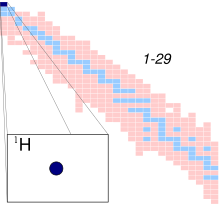
Symbol	1H
Names	hydrogen atom, H-1, protium
Protons (Z)	1
Neutrons (N)	0
Nuclide data
Natural abundance	99.985%
Half-life (t1/2)	stable
Isotope mass	1.007825 u
Spin	1/2
Excess energy	7288.969±0.001 keV
Binding energy	0.000±0.0000 keV
Isotopes of hydrogen Complete table of nuclides

Depiction of a hydrogen atom showing the diameter as about twice the Bohr model radius. (Image not to scale)

A hydrogen atom is an atom of the chemical element hydrogen. The electrically neutral atom contains a single positively charged proton and a single negatively charged electron bound to the nucleus by the Coulomb force. Atomic hydrogen constitutes about 75% of the baryonic mass of the universe.

In everyday life on Earth, isolated hydrogen atoms (called "atomic hydrogen") are extremely rare. Instead, a hydrogen atom tends to combine with other atoms in compounds, or with another hydrogen atom to form ordinary (diatomic) hydrogen gas, H₂. "Atomic hydrogen" and "hydrogen atom" in ordinary English use have overlapping, yet distinct, meanings. For example, a water molecule contains two hydrogen atoms, but does not contain atomic hydrogen (which would refer to isolated hydrogen atoms).

Atomic spectroscopy shows that there is a discrete infinite set of states in which a hydrogen (or any) atom can exist, contrary to the predictions of classical physics. Attempts to develop a theoretical understanding of the states of the hydrogen atom have been important to the history of quantum mechanics, since all other atoms can be roughly understood by knowing in detail about this simplest atomic structure.

Isotopes

Main article: Isotopes of hydrogen

The most abundant isotope, hydrogen-1, protium, or light hydrogen, contains no neutrons and is simply a proton and an electron. Protium is stable and makes up 99.985% of naturally occurring hydrogen atoms.

Deuterium contains one neutron and one proton in its nucleus. Deuterium is stable and makes up 0.0156% of naturally occurring hydrogen and is used in industrial processes like nuclear reactors and Nuclear Magnetic Resonance.

Tritium contains two neutrons and one proton in its nucleus and is not stable, decaying with a half-life of 12.32 years. Because of its short half-life, tritium does not exist in nature except in trace amounts.

Heavier isotopes of hydrogen are only created artificially in particle accelerators and have half-lives on the order of 10⁻²² seconds. They are unbound resonances located beyond the neutron drip line; this results in prompt emission of a neutron.

The formulas below are valid for all three isotopes of hydrogen, but slightly different values of the Rydberg constant (correction formula given below) must be used for each hydrogen isotope.

Hydrogen ion

Main articles: hydrogen cation and hydrogen anion

Lone neutral hydrogen atoms are rare under normal conditions. However, neutral hydrogen is common when it is covalently bound to another atom, and hydrogen atoms can also exist in cationic and anionic forms.

If a neutral hydrogen atom loses its electron, it becomes a cation. The resulting ion, which consists solely of a proton for the usual isotope, is written as "H⁺" and sometimes called hydron. Free protons are common in the interstellar medium, and solar wind. In the context of aqueous solutions of classical Brønsted–Lowry acids, such as hydrochloric acid, it is actually hydronium, H₃O⁺, that is meant. Instead of a literal ionized single hydrogen atom being formed, the acid transfers the hydrogen to H₂O, forming H₃O⁺.

If instead a hydrogen atom gains a second electron, it becomes an anion. The hydrogen anion is written as "H^–" and called hydride.

Theoretical analysis

The hydrogen atom has special significance in quantum mechanics and quantum field theory as a simple two-body problem physical system which has yielded many simple analytical solutions in closed-form.

Failed classical description

Experiments by Ernest Rutherford in 1909 showed the structure of the atom to be a dense, positive nucleus with a tenuous negative charge cloud around it. This immediately raised questions about how such a system could be stable. Classical electromagnetism had shown that any accelerating charge radiates energy, as shown by the Larmor formula. If the electron is assumed to orbit in a perfect circle and radiates energy continuously, the electron would rapidly spiral into the nucleus with a fall time of:

$${\displaystyle t_{\text{fall}}\approx {\frac {a_{0}^{3}}{4r_{0}^{2}c}}\approx 1.6\times 10^{-11}{\text{ s}},}$$

where ${\displaystyle a_{0}}$ is the Bohr radius and ${\displaystyle r_{0}}$ is the classical electron radius. If this were true, all atoms would instantly collapse, however atoms seem to be stable. Furthermore, the spiral inward would release a smear of electromagnetic frequencies as the orbit got smaller. Instead, atoms were observed to only emit discrete frequencies of radiation. The resolution would lie in the development of quantum mechanics.

Bohr–Sommerfeld Model

Main article: Bohr model

In 1913, Niels Bohr obtained the energy levels and spectral frequencies of the hydrogen atom after making a number of simple assumptions in order to correct the failed classical model. The assumptions included:

1. Electrons can only be in certain, discrete circular orbits or stationary states, thereby having a discrete set of possible radii and energies.
2. Electrons do not emit radiation while in one of these stationary states.
3. An electron can gain or lose energy by jumping from one discrete orbit to another.

Bohr supposed that the electron's angular momentum is quantized with possible values:

$${\displaystyle L=n\hbar }$$

where ${\displaystyle n=1,2,3,\ldots }$ and ${\displaystyle \hbar }$ is Planck constant over ${\displaystyle 2\pi }$. He also supposed that the centripetal force which keeps the electron in its orbit is provided by the Coulomb force, and that energy is conserved. Bohr derived the energy of each orbit of the hydrogen atom to be:

$${\displaystyle E_{n}=-{\frac {m_{e}e^{4}}{2(4\pi \varepsilon _{0})^{2}\hbar ^{2}}}{\frac {1}{n^{2}}},}$$

where ${\displaystyle m_{e}}$ is the electron mass, ${\displaystyle e}$ is the electron charge, ${\displaystyle \epsilon _{0}}$ is the vacuum permittivity, and ${\displaystyle n}$ is the quantum number (now known as the principal quantum number). Bohr's predictions matched experiments measuring the hydrogen spectral series to the first order, giving more confidence to a theory that used quantized values.

For ${\displaystyle n=1}$, the value

$${\displaystyle {\frac {m_{e}e^{4}}{2(4\pi \varepsilon _{0})^{2}\hbar ^{2}}}={\frac {m_{\text{e}}e^{4}}{8h^{2}\varepsilon _{0}^{2}}}=1\,{\text{Ry}}=13.605\;693\;122\;994(26)\,{\text{eV}}}$$

is called the Rydberg unit of energy. It is related to the Rydberg constant ${\displaystyle R_{\infty }}$ of atomic physics by ${\displaystyle 1\,{\text{Ry}}\equiv hcR_{\infty }.}$

The exact value of the Rydberg constant assumes that the nucleus is infinitely massive with respect to the electron. For hydrogen-1, hydrogen-2 (deuterium), and hydrogen-3 (tritium) which have finite mass, the constant must be slightly modified to use the reduced mass of the system, rather than simply the mass of the electron. This includes the kinetic energy of the nucleus in the problem, because the total (electron plus nuclear) kinetic energy is equivalent to the kinetic energy of the reduced mass moving with a velocity equal to the electron velocity relative to the nucleus. However, since the nucleus is much heavier than the electron, the electron mass and reduced mass are nearly the same. The Rydberg constant R_M for a hydrogen atom (one electron), R is given by

$${\displaystyle R_{M}={\frac {R_{\infty }}{1+m_{\text{e}}/M}},}$$

where ${\displaystyle M}$ is the mass of the atomic nucleus. For hydrogen-1, the quantity ${\displaystyle m_{\text{e}}/M,}$ is about 1/1836 (i.e. the electron-to-proton mass ratio). For deuterium and tritium, the ratios are about 1/3670 and 1/5497 respectively. These figures, when added to 1 in the denominator, represent very small corrections in the value of R, and thus only small corrections to all energy levels in corresponding hydrogen isotopes.

There were still problems with Bohr's model:

1. it failed to predict other spectral details such as fine structure and hyperfine structure
2. it could only predict energy levels with any accuracy for single–electron atoms (hydrogen–like atoms)
3. the predicted values were only correct to ${\displaystyle \alpha ^{2}\approx 10^{-5}}$, where ${\displaystyle \alpha }$ is the fine-structure constant.

Most of these shortcomings were resolved by Arnold Sommerfeld's modification of the Bohr model. Sommerfeld introduced two additional degrees of freedom, allowing an electron to move on an elliptical orbit characterized by its eccentricity and declination with respect to a chosen axis. This introduced two additional quantum numbers, which correspond to the orbital angular momentum and its projection on the chosen axis. Thus the correct multiplicity of states (except for the factor 2 accounting for the yet unknown electron spin) was found. Further, by applying special relativity to the elliptic orbits, Sommerfeld succeeded in deriving the correct expression for the fine structure of hydrogen spectra (which happens to be exactly the same as in the most elaborate Dirac theory). However, some observed phenomena, such as the anomalous Zeeman effect, remained unexplained. These issues were resolved with the full development of quantum mechanics and the Dirac equation. It is often alleged that the Schrödinger equation is superior to the Bohr–Sommerfeld theory in describing hydrogen atom. This is not the case, as most of the results of both approaches coincide or are very close (a remarkable exception is the problem of hydrogen atom in crossed electric and magnetic fields, which cannot be self-consistently solved in the framework of the Bohr–Sommerfeld theory), and in both theories the main shortcomings result from the absence of the electron spin. It was the complete failure of the Bohr–Sommerfeld theory to explain many-electron systems (such as helium atom or hydrogen molecule) which demonstrated its inadequacy in describing quantum phenomena.

Schrödinger equation

The Schrödinger equation allows one to calculate the stationary states and also the time evolution of quantum systems. Exact analytical answers are available for the nonrelativistic hydrogen atom. Before we go to present a formal account, here we give an elementary overview.

Given that the hydrogen atom contains a nucleus and an electron, quantum mechanics allows one to predict the probability of finding the electron at any given radial distance ${\displaystyle r}$. It is given by the square of a mathematical function known as the "wavefunction," which is a solution of the Schrödinger equation. The lowest energy equilibrium state of the hydrogen atom is known as the ground state. The ground state wave function is known as the ${\displaystyle 1\mathrm {s} }$ wavefunction. It is written as:

$${\displaystyle \psi _{1\mathrm {s} }(r)={\frac {1}{{\sqrt {\pi }}a_{0}^{3/2}}}e^{-r/a_{0}}.}$$

Here, ${\displaystyle a_{0}}$ is the numerical value of the Bohr radius. The probability density of finding the electron at a distance ${\displaystyle r}$ in any radial direction is the squared value of the wavefunction:

$${\displaystyle |\psi _{1\mathrm {s} }(r)|^{2}={\frac {1}{\pi a_{0}^{3}}}e^{-2r/a_{0}}.}$$

The ${\displaystyle 1\mathrm {s} }$ wavefunction is spherically symmetric, and the surface area of a shell at distance ${\displaystyle r}$ is ${\displaystyle 4\pi r^{2}}$, so the total probability ${\displaystyle P(r)\,dr}$ of the electron being in a shell at a distance ${\displaystyle r}$ and thickness ${\displaystyle dr}$ is

$${\displaystyle P(r)\,dr=4\pi r^{2}|\psi _{1\mathrm {s} }(r)|^{2}\,dr.}$$

It turns out that this is a maximum at ${\displaystyle r=a_{0}}$. That is, the Bohr picture of an electron orbiting the nucleus at radius ${\displaystyle a_{0}}$ corresponds to the most probable radius. Actually, there is a finite probability that the electron may be found at any place ${\displaystyle r}$, with the probability indicated by the square of the wavefunction. Since the probability of finding the electron somewhere in the whole volume is unity, the integral of ${\displaystyle P(r)\,dr}$ is unity. Then we say that the wavefunction is properly normalized.

As discussed below, the ground state ${\displaystyle 1\mathrm {s} }$ is also indicated by the quantum numbers ${\displaystyle (n=1,\ell =0,m=0)}$. The second lowest energy states, just above the ground state, are given by the quantum numbers ${\displaystyle (2,0,0)}$, ${\displaystyle (2,1,0)}$, and ${\displaystyle (2,1,\pm 1)}$. These ${\displaystyle n=2}$ states all have the same energy and are known as the ${\displaystyle 2\mathrm {s} }$ and ${\displaystyle 2\mathrm {p} }$ states. There is one ${\displaystyle 2\mathrm {s} }$ state:

$${\displaystyle \psi _{2,0,0}={\frac {1}{4{\sqrt {2\pi }}a_{0}^{3/2}}}\left(2-{\frac {r}{a_{0}}}\right)e^{-r/2a_{0}},}$$

and there are three ${\displaystyle 2\mathrm {p} }$ states:

$${\displaystyle \psi _{2,1,0}={\frac {1}{4{\sqrt {2\pi }}a_{0}^{3/2}}}{\frac {r}{a_{0}}}e^{-r/2a_{0}}\cos \theta ,}$$

$${\displaystyle \psi _{2,1,\pm 1}=\mp {\frac {1}{8{\sqrt {\pi }}a_{0}^{3/2}}}{\frac {r}{a_{0}}}e^{-r/2a_{0}}\sin \theta ~e^{\pm i\varphi }.}$$

An electron in the ${\displaystyle 2\mathrm {s} }$ or ${\displaystyle 2\mathrm {p} }$ state is most likely to be found in the second Bohr orbit with energy given by the Bohr formula.

Wavefunction

The Hamiltonian of the hydrogen atom is the radial kinetic energy operator and Coulomb attraction force between the positive proton and negative electron. Using the time-independent Schrödinger equation, ignoring all spin-coupling interactions and using the reduced mass ${\displaystyle \mu =m_{e}M/(m_{e}+M)}$, the equation is written as:

$${\displaystyle \left(-{\frac {\hbar ^{2}}{2\mu }}\nabla ^{2}-{\frac {e^{2}}{4\pi \varepsilon _{0}r}}\right)\psi (r,\theta ,\varphi )=E\psi (r,\theta ,\varphi )}$$

Expanding the Laplacian in spherical coordinates:

$${\displaystyle -{\frac {\hbar ^{2}}{2\mu }}\left[{\frac {1}{r^{2}}}{\frac {\partial }{\partial r}}\left(r^{2}{\frac {\partial \psi }{\partial r}}\right)+{\frac {1}{r^{2}\sin \theta }}{\frac {\partial }{\partial \theta }}\left(\sin \theta {\frac {\partial \psi }{\partial \theta }}\right)+{\frac {1}{r^{2}\sin ^{2}\theta }}{\frac {\partial ^{2}\psi }{\partial \varphi ^{2}}}\right]-{\frac {e^{2}}{4\pi \varepsilon _{0}r}}\psi =E\psi }$$

This is a separable, partial differential equation which can be solved in terms of special functions. When the wavefunction is separated as product of functions ${\displaystyle R(r)}$, ${\displaystyle \Theta (\theta )}$, and ${\displaystyle \Phi (\varphi )}$ three independent differential functions appears with A and B being the separation constants:

• radial:
  $${\displaystyle {\frac {d}{dr}}\left(r^{2}{\frac {dR}{dr}}\right)+{\frac {2\mu r^{2}}{\hbar ^{2}}}\left(E+{\frac {e^{2}}{4\pi \varepsilon _{0}r}}\right)R-AR=0}$$

  
• polar:
  $${\displaystyle {\frac {\sin \theta }{\Theta }}{\frac {d}{d\theta }}\left(\sin \theta {\frac {d\Theta }{d\theta }}\right)+A\sin ^{2}\theta -B=0}$$

  
• azimuth:
  $${\displaystyle {\frac {1}{\Phi }}{\frac {d^{2}\Phi }{d\varphi ^{2}}}+B=0.}$$

  

The normalized position wavefunctions, given in spherical coordinates are:

$${\displaystyle \psi _{n\ell m}(r,\theta ,\varphi )={\sqrt {{\left({\frac {2}{na_{0}^{*}}}\right)}^{3}{\frac {(n-\ell -1)!}{2n(n+\ell )!}}}}e^{-\rho /2}\rho ^{\ell }L_{n-\ell -1}^{2\ell +1}(\rho )Y_{\ell }^{m}(\theta ,\varphi )}$$

3D illustration of the eigenstate ${\displaystyle \psi _{4,3,1}}$. Electrons in this state are 45% likely to be found within the solid body shown.

where:

• ${\displaystyle \rho ={2r \over {na_{0}^{*}}}}$,
• ${\displaystyle a_{0}^{*}}$ is the reduced Bohr radius, ${\displaystyle a_{0}^{*}={{4\pi \varepsilon _{0}\hbar ^{2}} \over {\mu e^{2}}}}$,
• ${\displaystyle L_{n-\ell -1}^{2\ell +1}(\rho )}$ is a generalized Laguerre polynomial of degree ${\displaystyle n-\ell -1}$, and
• ${\displaystyle Y_{\ell }^{m}(\theta ,\varphi )}$ is a spherical harmonic function of degree ${\displaystyle \ell }$ and order ${\displaystyle m}$. Note that the generalized Laguerre polynomials are defined differently by different authors. The usage here is consistent with the definitions used by Messiah, and Mathematica. In other places, the Laguerre polynomial includes a factor of ${\displaystyle (n+\ell )!}$, or the generalized Laguerre polynomial appearing in the hydrogen wave function is ${\displaystyle L_{n+\ell }^{2\ell +1}(\rho )}$ instead.

The quantum numbers can take the following values:

• ${\displaystyle n=1,2,3,\ldots }$ (principal quantum number)
• ${\displaystyle \ell =0,1,2,\ldots ,n-1}$ (azimuthal quantum number)
• ${\displaystyle m=-\ell ,\ldots ,\ell }$ (magnetic quantum number).

Additionally, these wavefunctions are normalized (i.e., the integral of their modulus square equals 1) and orthogonal:

$${\displaystyle \int _{0}^{\infty }r^{2}\,dr\int _{0}^{\pi }\sin \theta \,d\theta \int _{0}^{2\pi }d\varphi \,\psi _{n\ell m}^{*}(r,\theta ,\varphi )\psi _{n'\ell 'm'}(r,\theta ,\varphi )=\langle n,\ell ,m|n',\ell ',m'\rangle =\delta _{nn'}\delta _{\ell \ell '}\delta _{mm'},}$$

where ${\displaystyle |n,\ell ,m\rangle }$ is the state represented by the wavefunction ${\displaystyle \psi _{n\ell m}}$ in Dirac notation, and ${\displaystyle \delta }$ is the Kronecker delta function.

The wavefunctions in momentum space are related to the wavefunctions in position space through a Fourier transform

$${\displaystyle \varphi (p,\theta _{p},\varphi _{p})=(2\pi \hbar )^{-3/2}\int e^{-i{\vec {p}}\cdot {\vec {r}}/\hbar }\psi (r,\theta ,\varphi )\,dV,}$$

which, for the bound states, results in

$${\displaystyle \varphi (p,\theta _{p},\varphi _{p})={\sqrt {{\frac {2}{\pi }}{\frac {(n-\ell -1)!}{(n+\ell )!}}}}n^{2}2^{2\ell +2}\ell !{\frac {n^{\ell }p^{\ell }}{(n^{2}p^{2}+1)^{\ell +2}}}C_{n-\ell -1}^{\ell +1}\left({\frac {n^{2}p^{2}-1}{n^{2}p^{2}+1}}\right)Y_{\ell }^{m}(\theta _{p},\varphi _{p}),}$$

where ${\displaystyle C_{N}^{\alpha }(x)}$ denotes a Gegenbauer polynomial and ${\displaystyle p}$ is in units of ${\displaystyle \hbar /a_{0}^{*}}$.

The solutions to the Schrödinger equation for hydrogen are analytical, giving a simple expression for the hydrogen energy levels and thus the frequencies of the hydrogen spectral lines and fully reproduced the Bohr model and went beyond it. It also yields two other quantum numbers and the shape of the electron's wave function ("orbital") for the various possible quantum-mechanical states, thus explaining the anisotropic character of atomic bonds.

The Schrödinger equation also applies to more complicated atoms and molecules. When there is more than one electron or nucleus the solution is not analytical and either computer calculations are necessary or simplifying assumptions must be made.

Since the Schrödinger equation is only valid for non-relativistic quantum mechanics, the solutions it yields for the hydrogen atom are not entirely correct. The Dirac equation of relativistic quantum theory improves these solutions (see below).

Results of Schrödinger equation

The solution of the Schrödinger equation (wave equation) for the hydrogen atom uses the fact that the Coulomb potential produced by the nucleus is isotropic (it is radially symmetric in space and only depends on the distance to the nucleus). Although the resulting energy eigenfunctions (the orbitals) are not necessarily isotropic themselves, their dependence on the angular coordinates follows completely generally from this isotropy of the underlying potential: the eigenstates of the Hamiltonian (that is, the energy eigenstates) can be chosen as simultaneous eigenstates of the angular momentum operator. This corresponds to the fact that angular momentum is conserved in the orbital motion of the electron around the nucleus. Therefore, the energy eigenstates may be classified by two angular momentum quantum numbers, ${\displaystyle \ell }$ and ${\displaystyle m}$ (both are integers). The angular momentum quantum number ${\displaystyle \ell =0,1,2,\ldots }$ determines the magnitude of the angular momentum. The magnetic quantum number ${\displaystyle m=-\ell ,\ldots ,+\ell }$ determines the projection of the angular momentum on the (arbitrarily chosen) ${\displaystyle z}$-axis.

In addition to mathematical expressions for total angular momentum and angular momentum projection of wavefunctions, an expression for the radial dependence of the wave functions must be found. It is only here that the details of the ${\displaystyle 1/r}$ Coulomb potential enter (leading to Laguerre polynomials in ${\displaystyle r}$). This leads to a third quantum number, the principal quantum number ${\displaystyle n=1,2,3,\ldots }$. The principal quantum number in hydrogen is related to the atom's total energy.

Note that the maximum value of the angular momentum quantum number is limited by the principal quantum number: it can run only up to ${\displaystyle n-1}$, i.e., ${\displaystyle \ell =0,1,\ldots ,n-1}$.

Due to angular momentum conservation, states of the same ${\displaystyle \ell }$ but different ${\displaystyle m}$ have the same energy (this holds for all problems with rotational symmetry). In addition, for the hydrogen atom, states of the same ${\displaystyle n}$ but different ${\displaystyle \ell }$ are also degenerate (i.e., they have the same energy). However, this is a specific property of hydrogen and is no longer true for more complicated atoms which have an (effective) potential differing from the form ${\displaystyle 1/r}$ (due to the presence of the inner electrons shielding the nucleus potential).

Taking into account the spin of the electron adds a last quantum number, the projection of the electron's spin angular momentum along the ${\displaystyle z}$-axis, which can take on two values. Therefore, any eigenstate of the electron in the hydrogen atom is described fully by four quantum numbers. According to the usual rules of quantum mechanics, the actual state of the electron may be any superposition of these states. This explains also why the choice of ${\displaystyle z}$-axis for the directional quantization of the angular momentum vector is immaterial: an orbital of given ${\displaystyle \ell }$ and ${\displaystyle m'}$ obtained for another preferred axis ${\displaystyle z'}$ can always be represented as a suitable superposition of the various states of different ${\displaystyle m}$ (but same ${\displaystyle \ell }$) that have been obtained for ${\displaystyle z}$.

Mathematical summary of eigenstates of hydrogen atom

Main article: Hydrogen-like atom

In 1928, Paul Dirac found an equation that was fully compatible with special relativity, and (as a consequence) made the wave function a 4-component "Dirac spinor" including "up" and "down" spin components, with both positive and "negative" energy (or matter and antimatter). The solution to this equation gave the following results, more accurate than the Schrödinger solution.

Energy levels

The energy levels of hydrogen, including fine structure (excluding Lamb shift and hyperfine structure), are given by the Sommerfeld fine structure expression:

$${\displaystyle {\begin{aligned}E_{j\,n}={}&-\mu c^{2}\left[1-\left(1+\left[{\frac {\alpha }{n-j-{\frac {1}{2}}+{\sqrt {\left(j+{\frac {1}{2}}\right)^{2}-\alpha ^{2}}}}}\right]^{2}\right)^{-1/2}\right]\\\approx {}&-{\frac {\mu c^{2}\alpha ^{2}}{2n^{2}}}\left[1+{\frac {\alpha ^{2}}{n^{2}}}\left({\frac {n}{j+{\frac {1}{2}}}}-{\frac {3}{4}}\right)\right],\end{aligned}}}$$

where ${\displaystyle \alpha }$ is the fine-structure constant and ${\displaystyle j}$ is the total angular momentum quantum number, which is equal to ${\displaystyle \left|\ell \pm {\tfrac {1}{2}}\right|}$, depending on the orientation of the electron spin relative to the orbital angular momentum. This formula represents a small correction to the energy obtained by Bohr and Schrödinger as given above. The factor in square brackets in the last expression is nearly one; the extra term arises from relativistic effects (for details, see #Features going beyond the Schrödinger solution). It is worth noting that this expression was first obtained by A. Sommerfeld in 1916 based on the relativistic version of the old Bohr theory. Sommerfeld has however used different notation for the quantum numbers.

Coherent states

The coherent states have been proposed as

$${\displaystyle |s,\gamma ,{\bar {\Omega }}\rangle \equiv M(s^{2})\sum _{n=0}^{\infty }(s^{n}e^{i\gamma /(n+1)^{2}}/{\sqrt {\rho _{n}}})|n,{\bar {\Omega }}\rangle ,}$$

which satisfies ${\displaystyle d{\bar {\Omega }}\equiv \sin {\bar {\theta }}\,d{\bar {\theta }}\,d{\bar {\varphi }}\,d{\bar {\psi }}/8\pi ^{2}}$ and takes the form

$${\displaystyle {\begin{aligned}\langle r,\theta ,\varphi \mid s,\gamma ,{\bar {\Omega }}\rangle ={}&e^{-s^{2}/2}\sum _{n=0}^{\infty }(s^{n}e^{i\gamma /(n+1)^{2}}/{\sqrt {n!}})\\&{}\times \,\sum _{\ell =0}^{n}u_{n+1}^{\ell }(r)\sum _{m=-\ell }^{\ell }\left[{\frac {(2\ell )!}{(\ell +m)!(\ell -m)!}}\right]^{1/2}\left(\sin {\frac {\bar {\theta }}{2}}\right)^{\ell -m}\left(\cos {\frac {\bar {\theta }}{2}}\right)^{\ell +m}\\&{}\times \,e^{-i(m{\bar {\varphi }}+\ell {\bar {\psi }})}Y_{\ell m}(\theta ,\varphi ){\sqrt {2\ell +1}}.\end{aligned}}}$$

Visualizing the hydrogen electron orbitals

Main article: Atomic orbital

 

Probability densities through the xz-plane for the electron at different quantum numbers (ℓ, across top; n, down side; m = 0)

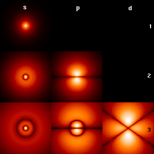
The image to the right shows the first few hydrogen atom orbitals (energy eigenfunctions). These are cross-sections of the probability density that are color-coded (black represents zero density and white represents the highest density). The angular momentum (orbital) quantum number ℓ is denoted in each column, using the usual spectroscopic letter code (s means ℓ = 0, p means ℓ = 1, d means ℓ = 2). The main (principal) quantum number n (= 1, 2, 3, ...) is marked to the right of each row. For all pictures the magnetic quantum number m has been set to 0, and the cross-sectional plane is the xz-plane (z is the vertical axis). The probability density in three-dimensional space is obtained by rotating the one shown here around the z-axis.

The "ground state", i.e. the state of lowest energy, in which the electron is usually found, is the first one, the 1s state (principal quantum level n = 1, ℓ = 0).

Black lines occur in each but the first orbital: these are the nodes of the wavefunction, i.e. where the probability density is zero. (More precisely, the nodes are spherical harmonics that appear as a result of solving the Schrödinger equation in spherical coordinates.)

The quantum numbers determine the layout of these nodes. There are:

• ${\displaystyle n-1}$ total nodes,
• ${\displaystyle \ell }$ of which are angular nodes:
  • ${\displaystyle m}$ angular nodes go around the ${\displaystyle \varphi }$ axis (in the xy plane). (The figure above does not show these nodes since it plots cross-sections through the xz-plane.)
  • ${\displaystyle \ell -m}$ (the remaining angular nodes) occur on the ${\displaystyle \theta }$ (vertical) axis.
• ${\displaystyle n-\ell -1}$ (the remaining non-angular nodes) are radial nodes.

Features going beyond the Schrödinger solution

There are several important effects that are neglected by the Schrödinger equation and which are responsible for certain small but measurable deviations of the real spectral lines from the predicted ones:

• Although the mean speed of the electron in hydrogen is only 1/137th of the speed of light, many modern experiments are sufficiently precise that a complete theoretical explanation requires a fully relativistic treatment of the problem. A relativistic treatment results in a momentum increase of about 1 part in 37,000 for the electron. Since the electron's wavelength is determined by its momentum, orbitals containing higher speed electrons show contraction due to smaller wavelengths.
• Even when there is no external magnetic field, in the inertial frame of the moving electron, the electromagnetic field of the nucleus has a magnetic component. The spin of the electron has an associated magnetic moment which interacts with this magnetic field. This effect is also explained by special relativity, and it leads to the so-called spin-orbit coupling, i.e., an interaction between the electron's orbital motion around the nucleus, and its spin.

Both of these features (and more) are incorporated in the relativistic Dirac equation, with predictions that come still closer to experiment. Again the Dirac equation may be solved analytically in the special case of a two-body system, such as the hydrogen atom. The resulting solution quantum states now must be classified by the total angular momentum number j (arising through the coupling between electron spin and orbital angular momentum). States of the same j and the same n are still degenerate. Thus, direct analytical solution of Dirac equation predicts 2S(1/2) and 2P(1/2) levels of hydrogen to have exactly the same energy, which is in a contradiction with observations (Lamb–Retherford experiment).

• There are always vacuum fluctuations of the electromagnetic field, according to quantum mechanics. Due to such fluctuations degeneracy between states of the same j but different l is lifted, giving them slightly different energies. This has been demonstrated in the famous Lamb–Retherford experiment and was the starting point for the development of the theory of quantum electrodynamics (which is able to deal with these vacuum fluctuations and employs the famous Feynman diagrams for approximations using perturbation theory). This effect is now called Lamb shift.

For these developments, it was essential that the solution of the Dirac equation for the hydrogen atom could be worked out exactly, such that any experimentally observed deviation had to be taken seriously as a signal of failure of the theory.

Alternatives to the Schrödinger theory

In the language of Heisenberg's matrix mechanics, the hydrogen atom was first solved by Wolfgang Pauli using a rotational symmetry in four dimensions [O(4)-symmetry] generated by the angular momentum and the Laplace–Runge–Lenz vector. By extending the symmetry group O(4) to the dynamical group O(4,2), the entire spectrum and all transitions were embedded in a single irreducible group representation.

In 1979 the (non-relativistic) hydrogen atom was solved for the first time within Feynman's path integral formulation of quantum mechanics by Duru and Kleinert. This work greatly extended the range of applicability of Feynman's method.

Pattern recognition

From Wikipedia, the free encyclopedia

https://en.wikipedia.org/wiki/Pattern_recognition

Pattern recognition is the automated recognition of patterns and regularities in data. It has applications in statistical data analysis, signal processing, image analysis, information retrieval, bioinformatics, data compression, computer graphics and machine learning. Pattern recognition has its origins in statistics and engineering; some modern approaches to pattern recognition include the use of machine learning, due to the increased availability of big data and a new abundance of processing power. These activities can be viewed as two facets of the same field of application, and they have undergone substantial development over the past few decades.

Pattern recognition systems are commonly trained from labeled "training" data. When no labeled data are available, other algorithms can be used to discover previously unknown patterns. KDD and data mining have a larger focus on unsupervised methods and stronger connection to business use. Pattern recognition focuses more on the signal and also takes acquisition and Signal Processing into consideration. It originated in engineering, and the term is popular in the context of computer vision: a leading computer vision conference is named Conference on Computer Vision and Pattern Recognition.

In machine learning, pattern recognition is the assignment of a label to a given input value. In statistics, discriminant analysis was introduced for this same purpose in 1936. An example of pattern recognition is classification, which attempts to assign each input value to one of a given set of classes (for example, determine whether a given email is "spam" or "non-spam"). Pattern recognition is a more general problem that encompasses other types of output as well. Other examples are regression, which assigns a real-valued output to each input; sequence labeling, which assigns a class to each member of a sequence of values (for example, part of speech tagging, which assigns a part of speech to each word in an input sentence); and parsing, which assigns a parse tree to an input sentence, describing the syntactic structure of the sentence.

Pattern recognition algorithms generally aim to provide a reasonable answer for all possible inputs and to perform "most likely" matching of the inputs, taking into account their statistical variation. This is opposed to pattern matching algorithms, which look for exact matches in the input with pre-existing patterns. A common example of a pattern-matching algorithm is regular expression matching, which looks for patterns of a given sort in textual data and is included in the search capabilities of many text editors and word processors.

Overview

A modern definition of pattern recognition is:

The field of pattern recognition is concerned with the automatic discovery of regularities in data through the use of computer algorithms and with the use of these regularities to take actions such as classifying the data into different categories.

Pattern recognition is generally categorized according to the type of learning procedure used to generate the output value. Supervised learning assumes that a set of training data (the training set) has been provided, consisting of a set of instances that have been properly labeled by hand with the correct output. A learning procedure then generates a model that attempts to meet two sometimes conflicting objectives: Perform as well as possible on the training data, and generalize as well as possible to new data (usually, this means being as simple as possible, for some technical definition of "simple", in accordance with Occam's Razor, discussed below). Unsupervised learning, on the other hand, assumes training data that has not been hand-labeled, and attempts to find inherent patterns in the data that can then be used to determine the correct output value for new data instances. A combination of the two that has been explored is semi-supervised learning, which uses a combination of labeled and unlabeled data (typically a small set of labeled data combined with a large amount of unlabeled data). In cases of unsupervised learning, there may be no training data at all.

Sometimes different terms are used to describe the corresponding supervised and unsupervised learning procedures for the same type of output. The unsupervised equivalent of classification is normally known as clustering, based on the common perception of the task as involving no training data to speak of, and of grouping the input data into clusters based on some inherent similarity measure (e.g. the distance between instances, considered as vectors in a multi-dimensional vector space), rather than assigning each input instance into one of a set of pre-defined classes. In some fields, the terminology is different. In community ecology, the term classification is used to refer to what is commonly known as "clustering".

The piece of input data for which an output value is generated is formally termed an instance. The instance is formally described by a vector of features, which together constitute a description of all known characteristics of the instance. These feature vectors can be seen as defining points in an appropriate multidimensional space, and methods for manipulating vectors in vector spaces can be correspondingly applied to them, such as computing the dot product or the angle between two vectors. Features typically are either categorical (also known as nominal, i.e., consisting of one of a set of unordered items, such as a gender of "male" or "female", or a blood type of "A", "B", "AB" or "O"), ordinal (consisting of one of a set of ordered items, e.g., "large", "medium" or "small"), integer-valued (e.g., a count of the number of occurrences of a particular word in an email) or real-valued (e.g., a measurement of blood pressure). Often, categorical and ordinal data are grouped together, and this is also the case for integer-valued and real-valued data. Many algorithms work only in terms of categorical data and require that real-valued or integer-valued data be discretized into groups (e.g., less than 5, between 5 and 10, or greater than 10).

Probabilistic classifiers

Main article: Probabilistic classifier

Many common pattern recognition algorithms are probabilistic in nature, in that they use statistical inference to find the best label for a given instance. Unlike other algorithms, which simply output a "best" label, often probabilistic algorithms also output a probability of the instance being described by the given label. In addition, many probabilistic algorithms output a list of the N-best labels with associated probabilities, for some value of N, instead of simply a single best label. When the number of possible labels is fairly small (e.g., in the case of classification), N may be set so that the probability of all possible labels is output. Probabilistic algorithms have many advantages over non-probabilistic algorithms:

• They output a confidence value associated with their choice. (Note that some other algorithms may also output confidence values, but in general, only for probabilistic algorithms is this value mathematically grounded in probability theory. Non-probabilistic confidence values can in general not be given any specific meaning, and only used to compare against other confidence values output by the same algorithm.)
• Correspondingly, they can abstain when the confidence of choosing any particular output is too low.
• Because of the probabilities output, probabilistic pattern-recognition algorithms can be more effectively incorporated into larger machine-learning tasks, in a way that partially or completely avoids the problem of error propagation.

Number of important feature variables

Feature selection algorithms attempt to directly prune out redundant or irrelevant features. A general introduction to feature selection which summarizes approaches and challenges, has been given. The complexity of feature-selection is, because of its non-monotonous character, an optimization problem where given a total of ${\displaystyle n}$ features the powerset consisting of all ${\displaystyle 2^{n}-1}$ subsets of features need to be explored. The Branch-and-Bound algorithm does reduce this complexity but is intractable for medium to large values of the number of available features ${\displaystyle n}$

Techniques to transform the raw feature vectors (feature extraction) are sometimes used prior to application of the pattern-matching algorithm. Feature extraction algorithms attempt to reduce a large-dimensionality feature vector into a smaller-dimensionality vector that is easier to work with and encodes less redundancy, using mathematical techniques such as principal components analysis (PCA). The distinction between feature selection and feature extraction is that the resulting features after feature extraction has taken place are of a different sort than the original features and may not easily be interpretable, while the features left after feature selection are simply a subset of the original features.

Problem statement

The problem of pattern recognition can be stated as follows: Given an unknown function ${\displaystyle g:{\mathcal {X}}\rightarrow {\mathcal {Y}}}$ (the ground truth) that maps input instances ${\displaystyle {\boldsymbol {x}}\in {\mathcal {X}}}$ to output labels ${\displaystyle y\in {\mathcal {Y}}}$, along with training data ${\displaystyle \mathbf {D} =\{({\boldsymbol {x}}_{1},y_{1}),\dots ,({\boldsymbol {x}}_{n},y_{n})\}}$ assumed to represent accurate examples of the mapping, produce a function ${\displaystyle h:{\mathcal {X}}\rightarrow {\mathcal {Y}}}$ that approximates as closely as possible the correct mapping ${\displaystyle g}$. (For example, if the problem is filtering spam, then ${\displaystyle {\boldsymbol {x}}_{i}}$ is some representation of an email and ${\displaystyle y}$ is either "spam" or "non-spam"). In order for this to be a well-defined problem, "approximates as closely as possible" needs to be defined rigorously. In decision theory, this is defined by specifying a loss function or cost function that assigns a specific value to "loss" resulting from producing an incorrect label. The goal then is to minimize the expected loss, with the expectation taken over the probability distribution of ${\displaystyle {\mathcal {X}}}$. In practice, neither the distribution of ${\displaystyle {\mathcal {X}}}$ nor the ground truth function ${\displaystyle g:{\mathcal {X}}\rightarrow {\mathcal {Y}}}$ are known exactly, but can be computed only empirically by collecting a large number of samples of ${\displaystyle {\mathcal {X}}}$ and hand-labeling them using the correct value of ${\displaystyle {\mathcal {Y}}}$ (a time-consuming process, which is typically the limiting factor in the amount of data of this sort that can be collected). The particular loss function depends on the type of label being predicted. For example, in the case of classification, the simple zero-one loss function is often sufficient. This corresponds simply to assigning a loss of 1 to any incorrect labeling and implies that the optimal classifier minimizes the error rate on independent test data (i.e. counting up the fraction of instances that the learned function ${\displaystyle h:{\mathcal {X}}\rightarrow {\mathcal {Y}}}$ labels wrongly, which is equivalent to maximizing the number of correctly classified instances). The goal of the learning procedure is then to minimize the error rate (maximize the correctness) on a "typical" test set.

For a probabilistic pattern recognizer, the problem is instead to estimate the probability of each possible output label given a particular input instance, i.e., to estimate a function of the form

${\displaystyle p({\rm {label}}|{\boldsymbol {x}},{\boldsymbol {\theta }})=f\left({\boldsymbol {x}};{\boldsymbol {\theta }}\right)}$

where the feature vector input is ${\displaystyle {\boldsymbol {x}}}$, and the function f is typically parameterized by some parameters ${\displaystyle {\boldsymbol {\theta }}}$.^[8] In a discriminative approach to the problem, f is estimated directly. In a generative approach, however, the inverse probability ${\displaystyle p({{\boldsymbol {x}}|{\rm {label}}})}$ is instead estimated and combined with the prior probability ${\displaystyle p({\rm {label}}|{\boldsymbol {\theta }})}$ using Bayes' rule, as follows:

${\displaystyle p({\rm {label}}|{\boldsymbol {x}},{\boldsymbol {\theta }})={\frac {p({{\boldsymbol {x}}|{\rm {label,{\boldsymbol {\theta }}}}})p({\rm {label|{\boldsymbol {\theta }}}})}{\sum _{L\in {\text{all labels}}}p({\boldsymbol {x}}|L)p(L|{\boldsymbol {\theta }})}}.}$

When the labels are continuously distributed (e.g., in regression analysis), the denominator involves integration rather than summation:

${\displaystyle p({\rm {label}}|{\boldsymbol {x}},{\boldsymbol {\theta }})={\frac {p({{\boldsymbol {x}}|{\rm {label,{\boldsymbol {\theta }}}}})p({\rm {label|{\boldsymbol {\theta }}}})}{\int _{L\in {\text{all labels}}}p({\boldsymbol {x}}|L)p(L|{\boldsymbol {\theta }})\operatorname {d} L}}.}$

The value of ${\displaystyle {\boldsymbol {\theta }}}$ is typically learned using maximum a posteriori (MAP) estimation. This finds the best value that simultaneously meets two conflicting objects: To perform as well as possible on the training data (smallest error-rate) and to find the simplest possible model. Essentially, this combines maximum likelihood estimation with a regularization procedure that favors simpler models over more complex models. In a Bayesian context, the regularization procedure can be viewed as placing a prior probability ${\displaystyle p({\boldsymbol {\theta }})}$ on different values of ${\displaystyle {\boldsymbol {\theta }}}$. Mathematically:

${\displaystyle {\boldsymbol {\theta }}^{*}=\arg \max _{\boldsymbol {\theta }}p({\boldsymbol {\theta }}|\mathbf {D} )}$

where ${\displaystyle {\boldsymbol {\theta }}^{*}}$ is the value used for ${\displaystyle {\boldsymbol {\theta }}}$ in the subsequent evaluation procedure, and ${\displaystyle p({\boldsymbol {\theta }}|\mathbf {D} )}$, the posterior probability of ${\displaystyle {\boldsymbol {\theta }}}$, is given by

${\displaystyle p({\boldsymbol {\theta }}|\mathbf {D} )=\left[\prod _{i=1}^{n}p(y_{i}|{\boldsymbol {x}}_{i},{\boldsymbol {\theta }})\right]p({\boldsymbol {\theta }}).}$

In the Bayesian approach to this problem, instead of choosing a single parameter vector ${\displaystyle {\boldsymbol {\theta }}^{*}}$, the probability of a given label for a new instance ${\displaystyle {\boldsymbol {x}}}$ is computed by integrating over all possible values of ${\displaystyle {\boldsymbol {\theta }}}$, weighted according to the posterior probability:

${\displaystyle p({\rm {label}}|{\boldsymbol {x}})=\int p({\rm {label}}|{\boldsymbol {x}},{\boldsymbol {\theta }})p({\boldsymbol {\theta }}|\mathbf {D} )\operatorname {d} {\boldsymbol {\theta }}.}$

Frequentist or Bayesian approach to pattern recognition

The first pattern classifier – the linear discriminant presented by Fisher – was developed in the frequentist tradition. The frequentist approach entails that the model parameters are considered unknown, but objective. The parameters are then computed (estimated) from the collected data. For the linear discriminant, these parameters are precisely the mean vectors and the covariance matrix. Also the probability of each class ${\displaystyle p({\rm {label}}|{\boldsymbol {\theta }})}$ is estimated from the collected dataset. Note that the usage of 'Bayes rule' in a pattern classifier does not make the classification approach Bayesian.

Bayesian statistics has its origin in Greek philosophy where a distinction was already made between the 'a priori' and the 'a posteriori' knowledge. Later Kant defined his distinction between what is a priori known – before observation – and the empirical knowledge gained from observations. In a Bayesian pattern classifier, the class probabilities ${\displaystyle p({\rm {label}}|{\boldsymbol {\theta }})}$ can be chosen by the user, which are then a priori. Moreover, experience quantified as a priori parameter values can be weighted with empirical observations – using e.g., the Beta- (conjugate prior) and Dirichlet-distributions. The Bayesian approach facilitates a seamless intermixing between expert knowledge in the form of subjective probabilities, and objective observations.

Probabilistic pattern classifiers can be used according to a frequentist or a Bayesian approach.

Uses

The face was automatically detected by special software.

Within medical science, pattern recognition is the basis for computer-aided diagnosis (CAD) systems. CAD describes a procedure that supports the doctor's interpretations and findings. Other typical applications of pattern recognition techniques are automatic speech recognition, speaker identification, classification of text into several categories (e.g., spam or non-spam email messages), the automatic recognition of handwriting on postal envelopes, automatic recognition of images of human faces, or handwriting image extraction from medical forms. The last two examples form the subtopic image analysis of pattern recognition that deals with digital images as input to pattern recognition systems.

Optical character recognition is an example of the application of a pattern classifier. The method of signing one's name was captured with stylus and overlay starting in 1990. The strokes, speed, relative min, relative max, acceleration and pressure is used to uniquely identify and confirm identity. Banks were first offered this technology, but were content to collect from the FDIC for any bank fraud and did not want to inconvenience customers.

Pattern recognition has many real-world applications in image processing. Some examples include:

• identification and authentication: e.g., license plate recognition, fingerprint analysis, face detection/verification, and voice-based authentication.
• medical diagnosis: e.g., screening for cervical cancer (Papnet), breast tumors or heart sounds;
• defense: various navigation and guidance systems, target recognition systems, shape recognition technology etc.
• mobility: advanced driver assistance systems, autonomous vehicle technology, etc.

In psychology, pattern recognition is used to make sense of and identify objects, and is closely related to perception. This explains how the sensory inputs humans receive are made meaningful. Pattern recognition can be thought of in two different ways. The first concerns template matching and the second concerns feature detection. A template is a pattern used to produce items of the same proportions. The template-matching hypothesis suggests that incoming stimuli are compared with templates in the long-term memory. If there is a match, the stimulus is identified. Feature detection models, such as the Pandemonium system for classifying letters (Selfridge, 1959), suggest that the stimuli are broken down into their component parts for identification. One observation is a capital E having three horizontal lines and one vertical line.

Algorithms

Algorithms for pattern recognition depend on the type of label output, on whether learning is supervised or unsupervised, and on whether the algorithm is statistical or non-statistical in nature. Statistical algorithms can further be categorized as generative or discriminative.

Classification methods (methods predicting categorical labels)

Main article: Statistical classification

Parametric:

• Linear discriminant analysis
• Quadratic discriminant analysis
• Maximum entropy classifier (aka logistic regression, multinomial logistic regression): Note that logistic regression is an algorithm for classification, despite its name. (The name comes from the fact that logistic regression uses an extension of a linear regression model to model the probability of an input being in a particular class.)

Nonparametric:

• Decision trees, decision lists
• Kernel estimation and K-nearest-neighbor algorithms
• Naive Bayes classifier
• Neural networks (multi-layer perceptrons)
• Perceptrons
• Support vector machines
• Gene expression programming

Clustering methods (methods for classifying and predicting categorical labels)

Main article: Cluster analysis

• Categorical mixture models
• Hierarchical clustering (agglomerative or divisive)
• K-means clustering
• Correlation clustering
• Kernel principal component analysis (Kernel PCA)

Ensemble learning algorithms (supervised meta-algorithms for combining multiple learning algorithms together)

Main article: Ensemble learning

• Boosting (meta-algorithm)
• Bootstrap aggregating ("bagging")
• Ensemble averaging
• Mixture of experts, hierarchical mixture of experts

General methods for predicting arbitrarily-structured (sets of) labels

• Bayesian networks
• Markov random fields

Multilinear subspace learning algorithms (predicting labels of multidimensional data using tensor representations)

Unsupervised:

• Multilinear principal component analysis (MPCA)

Real-valued sequence labeling methods (predicting sequences of real-valued labels)

Main article: sequence labeling

• Kalman filters
• Particle filters

Regression methods (predicting real-valued labels)

Main article: Regression analysis

• Gaussian process regression (kriging)
• Linear regression and extensions
• Independent component analysis (ICA)
• Principal components analysis (PCA)

Sequence labeling methods (predicting sequences of categorical labels)

• Conditional random fields (CRFs)
• Hidden Markov models (HMMs)
• Maximum entropy Markov models (MEMMs)
• Recurrent neural networks (RNNs)
• Dynamic time warping (DTW)