Search This Blog

Wednesday, August 31, 2022

Total fertility rate

From Wikipedia, the free encyclopedia

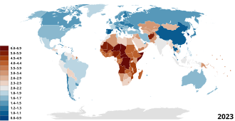
Map of countries by fertility rate (2020), according to the Population Reference Bureau

The total fertility rate (TFR) of a population is the average number of children that would be born to a woman over her lifetime if:

  1. she were to experience the exact current age-specific fertility rates (ASFRs) through her lifetime
  2. she were to live from birth until the end of her reproductive life.

It is obtained by summing the single-year age-specific rates at a given time. As of 2021, the total fertility rate varied from 0.81 in South Korea to 6.91 in Niger.

Fertility tends to be correlated with the level of economic development. Historically, developed countries usually have a significantly lower fertility rate, generally correlated with greater wealth, education, urbanization, and other factors. Conversely, in undeveloped countries, fertility rates tend to be higher. Families desire children for their labor and as caregivers for their parents in old age. Fertility rates are also higher due to the lack of access to contraceptives, stricter adherence to traditional religious beliefs, generally lower levels of female education, and lower rates of female employment.

The total fertility rate for the world today (2019) is 2.4. Global TFR has been declining rapidly since the 1960s, and some forecasters like Sanjeev Sanyal argue that the effective global fertility rate will fall below replacement rate, estimated to be 2.3, in the 2020s. This would stabilize world population sometime during the period 2050-2070. This differs from projections by the United Nations which estimates that some growth in world population will continue even up to 2100. Taken together, these projections imply that the population of this planet will reach zero growth sometime in the second half of this century.

Parameter characteristics

The TFR is not based on the fertility of any real group of women since this would involve waiting until they had completed childbearing. Nor is it based on counting up the total number of children actually born over their lifetime. Instead, the TFR is based on the age-specific fertility rates of women in their "child-bearing years", which in conventional international statistical usage is ages 15–44.

The TFR is, therefore, a measure of the fertility of an imaginary woman who passes through her reproductive life subject to all the age-specific fertility rates for ages 15–49 that were recorded for a given population in a given year. The TFR represents the average number of children a woman would potentially have, were she to fast-forward through all her childbearing years in a single year, under all the age-specific fertility rates for that year. In other words, this rate is the number of children a woman would have if she was subject to prevailing fertility rates at all ages from a single given year and survives throughout all her childbearing years.

Related parameters

Net reproduction rate

An alternative fertility measure is the net reproduction rate (NRR), which measures the number of daughters a woman would have in her lifetime if she were subject to prevailing age-specific fertility and mortality rates in the given year. When the NRR is exactly 1, then each generation of women is exactly reproducing itself.

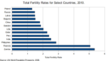
Total fertility rate for selected countries

The NRR is less widely used than the TFR, and the United Nations stopped reporting NRR data for member nations after 1998. But the NRR is particularly relevant where the number of male babies born is very high due to gender imbalance and sex selection. This is a significant factor in world population, due to the high level of gender imbalance in the very populous nations of China and India. The gross reproduction rate (GRR), is the same as the NRR, except that—like the TFR—it ignores life expectancy.

Total period fertility rate

The TFR (or TPFR—total period fertility rate) is a better index of fertility than the crude birth rate (annual number of births per thousand population) because it is independent of the age structure of the population, but it is a poorer estimate of actual completed family size than the total cohort fertility rate, which is obtained by summing the age-specific fertility rates that actually applied to each cohort as they aged through time. In particular, the TFR does not necessarily predict how many children young women now will eventually have, as their fertility rates in years to come may change from those of older women now. However, the TFR is a reasonable summary of current fertility levels. TFR and long term population growth rate, g, are closely related. For a population structure in a steady state, growth rate equals log(TFR/2)/Xm, where Xm is the mean age for childbearing women.

Tempo effect

The TPFR (total period fertility rate) is affected by a tempo effect—if age of childbearing increases (and life cycle fertility is unchanged) then while the age of childbearing is increasing, TPFR will be lower (because the births are occurring later), and then the age of childbearing stops increasing, the TPFR will increase (due to the deferred births occurring in the later period) even though the life cycle fertility has been unchanged. In other words, the TPFR is a misleading measure of life cycle fertility when childbearing age is changing, due to this statistical artifact. This is a significant factor in some countries, such as the Czech Republic and Spain in the 1990s. Some measures seek to adjust for this timing effect to gain a better measure of life-cycle fertility.

Replacement rates

Replacement fertility is the total fertility rate at which women give birth to enough babies to sustain population levels, assuming that mortality rates remain constant and net migration is zero. If replacement level fertility is sustained over a sufficiently long period, each generation will exactly replace itself. The replacement fertility rate is 2.1 births per woman for most developed countries (2.1 in the UK, for example), but can be as high as 3.5 in undeveloped countries because of higher mortality rates, especially child mortality. The global average for the replacement total fertility rate (eventually leading to a stable global population) for the contemporary period (2010-2015) is 2.3 children per woman.

Lowest-low fertility

The term "lowest-low fertility" is defined as TFR at or below 1.3. This is characteristic of some Eastern European, Southern European, and East Asian countries. For example, in 2001, more than half of the population of Europe lived in countries with the lowest-low TFR, although TFRs there have increased slightly since then.

The lowest TFR recorded anywhere in the world in recorded history is for Xiangyang district of Jiamusi city (Heilongjiang, China) which had a TFR of 0.41. Outside China, the lowest TFR ever recorded was 0.80 for Eastern Germany in 1994. The low Eastern German value was influenced by a change to higher age at birth, with the consequence that neither older cohorts (e.g. women born until the late 1960s), who often already had children, nor younger cohorts, who were postponing childbirth, had many children during that time. The total cohort fertility rate of each age cohort of women in East German did not drop as significantly.

Population-lag effect

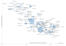
A plot of population growth rate vs total fertility rate (logarithmic). Symbol radius reflect population size in each country

A population that maintained a TFR of 3.8 over an extended period without a correspondingly high death or emigration rate would increase rapidly (doubling period ~ 32 years), whereas a population that maintained a TFR of 2.0 over a long time would decrease, unless it had a large enough immigration. However, it may take several generations for a change in the total fertility rate to be reflected in birth rate, because the age distribution must reach equilibrium. For example, a population that has recently dropped below replacement-level fertility will continue to grow, because the recent high fertility produced large numbers of young couples who would now be in their childbearing years.

This phenomenon carries forward for several generations and is called population momentum, population inertia, or population-lag effect. This time-lag effect is of great importance to the growth rates of human populations.

TFR (net) and long-term population growth rate, g, are closely related. For a population structure in a steady state and with zero migration, g equals log(TFR/2)/Xm, where Xm is mean age for childbearing women and thus P(t) = P(0)exp(gt). At the left side is shown the empirical relation between the two variables in a cross-section of countries with the most recent y-y growth rate. The parameter 1/b should be an estimate of the Xm; here equal to 1/0.02 = 50 years, way off the mark because of population momentum. E.g. for log(TFR/2) = 0, g should be exactly zero, which is seen not to be the case.

Factors affecting total fertility rate

Fertility factors are determinants of the number of children that an individual is likely to have. Fertility factors are mostly positive or negative correlations without certain causations.

Factors generally associated with increased fertility include the intention to have children, very high level of gender equality, religiosity, inter-generational transmission of values, marriage and cohabitation, maternal and social support, rural residence, pro family government programs, low IQ and increased food production.

Total Fertility Rate vs Human Development Index for Selected Countries

Factors generally associated with decreased fertility include rising income, value and attitude changes, education, female labor participation, population control, age, contraception, partner reluctance to having children, a low level of gender equality, and infertility.

Niger has the highest TFR in the world at 6.9 (2021 estimate)

The effect of all these factors can be summarized with a plot of Total Fertility Rate against Human Development Index (HDI) for a sample of countries. The chart shows that the two factors are inversely correlated, that is, in general, the lower a country’s HDI the higher its fertility.

Another common way of summarizing the relationship between economic development and fertility is a plot of TFR against Per Capita GDP, a proxy for standard of living. This chart shows that Per Capita GDP is also inversely correlated with fertility.

The impact of human development on TFR can best be summarized by a quote from Karan Singh, a former minister of population in India.  At a 1974 United Nations population conference in Bucharest, he said "Development is the best contraceptive."

Total Fertility Rate vs Per Capita GDP For Selected Countries. Population size shown as bubble area, (2016 estimates; 30 largest countries bold).

Wealthy countries, those with high per capita GDP, usually have a lower fertility rate than poor countries, those with low per capita GDP. This may seem counter-intuitive. The inverse relationship between income and fertility has been termed a demographic-economic paradox because evolutionary biology suggests that greater means should enable the production of more offspring, not fewer.

Many of these factors, however, are not universal, and differ by region and social class. For instance, at a global level, religion is correlated with increased fertility, but in the West less so: Scandinavian countries and France are among the least religious in the EU, but have the highest TFR, while the opposite is true about Portugal, Greece, Cyprus, Poland and Spain.

National efforts to increase or decrease fertility

Governments have often set population targets, to either increase or decrease the total fertility rate; or to have certain ethnic or socioeconomic groups have a lower or higher fertility rate. Often such policies have been interventionist, and abusive. The most notorious natalist policies of the 20th century include those in communist Romania and communist Albania, under Nicolae Ceaușescu and Enver Hoxha respectively. The policy of Romania (1967–1990) was very aggressive, including outlawing abortion and contraception, routine pregnancy tests for women, taxes on childlessness, and legal discrimination against childless people; and resulted in large numbers of children put into Romanian orphanages by parents who couldn't cope with raising them, street children in the 1990s (when many orphanages were closed and the children ended up on the streets), overcrowding in homes and schools, and over 9,000 women who died due to illegal abortions. Conversely, in China the government sought to lower the fertility rate, and, as such, enacted the one-child policy (1978–2015), which included abuses such as forced abortions.

Some governments have sought to regulate which groups of society could reproduce through eugenic policies of forced sterilizations of 'undesirable' population groups. Such policies were carried out against ethnic minorities in Europe and North America in the first half of the 20th century, and more recently in Latin America against the Indigenous population in the 1990s; in Peru, President Alberto Fujimori (in office from 1990 to 2000) has been accused of genocide and crimes against humanity as a result of a sterilization program put in place by his administration targeting indigenous people (mainly the Quechuas and the Aymaras). Within these historical contexts, the notion of reproductive rights has developed. Such rights are based on the concept that each person freely decides if, when, and how many children to have - not the state or church. According to the OHCHR reproductive rights "rest on the recognition of the basic rights of all couples and individuals to decide freely and responsibly the number, spacing and timing of their children and to have the information and means to do so, and the right to attain the highest standard of sexual and reproductive health. It also includes the right to make decisions concerning reproduction free of discrimination, coercion and violence, as expressed in human rights documents".

History of total fertility rate and projections for the future

From around 10,000 BC to the beginning of the Industrial Revolution fertility rates around the world were high by today's standards, but the onset of the Industrial Revolution, around 1800, brought about what has come to be called the Demographic Transition, and TFR began a long-term decline in almost every region of the world, a decline that continues to this day.

Before 1800

Because all nations before the Industrial Revolution were caught in what is now labeled the "Malthusian Trap", improvements in standards of living could only be achieved by reductions in population growth through either increases in mortality rates (via wars, plagues, famines, etc) or reductions in birth rates. However, at the same time, other realities such as child mortality, that could reach 50%, and the need to produce workers, male heirs, and old-age care givers required fertility rates to be high by today’s standards.

For example, fertility rates in Europe in the years before 1800 ranged from 4.5 (Scandinavia) to 6.2 (Belgium). The Total Fertility Rate in America in 1800 was 7.0. Fertility rates in Asia during this period were similar to those in Europe. In spite of these high fertility rates, global population growth was still very slow, about 0.04% per year, mostly due to high mortality rates and the equally slow growth in the production of food.

1800 to 1950

After 1800 the Industrial Revolution got underway in some countries, particularly Great Britain, other countries in Europe, and the United States, and they underwent the beginnings of what is now called the Demographic Transition. Stage two of this process fueled a steady reduction in mortality rates due to, for example, improvements in public sanitation, personal hygiene and the food supply (that, for example, reduced the number of famines).

These reductions in mortality rates, particularly reductions in child mortality that increased the fraction of children surviving, plus other major societal changes such as urbanization, then led to stage three of the Demographic Transition and a reduction in fertility rates because there was simply no longer a need to birth so many children.

The example from the US of the correlation between child mortality and the fertility rate is illustrative. In 1800 child mortality in the US was 33%. That is, one third of all children born would die before their fifth birthday. The Total Fertility Rate in 1800 was 7.0, meaning that the average woman would bear seven children during her lifetime. One hundred years later, in 1900, child mortality in the US had declined to 23%, a reduction of almost one third, and TFR had declined to 3.9, a reduction of 44%. By 1950, just fifty years later, child mortality had declined dramatically to 4%, a reduction of 84%, and TFR had declined to 3.2. By 2018 child mortality had declined further to 0.6% and TFR had declined further to 1.9, below replacement level.

1950 to the present and projections

Total fertility rate projections by region

The table shows that after 1965 the Demographic Transition had spread around the world and global TFR began a long decline that continues to this day.

World historical TFR (1950–2020)
Years TFR
1950–1955 4.96
1955–1960 4.89
1960–1965 5.03
1965–1970 4.92
1970–1975 4.46
1975–1980 3.87
1980–1985 3.59
1985–1990 3.44
1990–1995 3.02
1995–2000 2.75
2000–2005 2.63
2005–2010 2.57
2010–2015 2.52
2015–2020 2.47

Global TFR today (2019) is 2.4. Because global fertility replacement rate for the contemporary period (2010–2015) has been estimated to be 2.3, humanity is therefore approaching a major milestone.

The chart shows that the decline in TFR since the 1960s has occurred in every region of the world and that the global TFR is projected to continue to decline for the remainder of this century.

Total fertility rate by region

The United Nations Population Division divides the world into six geographic regions. The table below shows the estimated TFR for each.

Region TFR

(2015-2020)

Africa 4.4
Asia 2.2
Europe 1.6
Latin America and Caribbean 2.0
North America 1.8
Oceania 2.4

Africa

This region has a TFR of 4.4, the highest in the world. Niger, Angola, Congo, Mali, and Chad are the highest. The most populous country in Africa, Nigeria, had an estimated TFR of 4.7 in 2021. The second most populous country, Ethiopia, had an estimated TFR of 4.1 in 2021.

The poverty of the region, and the high maternal mortality and infant mortality had led to calls from WHO of family planning and encouragement of smaller families.

South Asia

India

The Indian fertility rate has declined significantly over the early 21st century. The Indian TFR declined from 5.2 in 1971 to 2.2 in 2018. According to recent surveys, TFR in India has further declined to 2.0 in 2021, marking the first time it has gone below replacement level.

Bangladesh

The fertility rate fell from 6.9 during the years 1970-75 to 2.0 in 2020, an interval of about 47 years, or a little more than one generation.

East Asia

Map of East Asia by total fertility rate (TFR) in 2021

Singapore, Macau, Taiwan, Hong Kong, and South Korea have lowest-low fertility, defined as TFR at or below 1.3, and are among the lowest in the world. Macau had a TFR below 1.0 in 2004. North Korea has the highest TFR in East Asia at 1.95.

China

The TFR of China was 1.15 in 2021. China implemented the one-child policy in 1979 as a drastic population planning measure to control the ever-growing population at the time. In 2015, the policy was replaced with two-child policy as China's population is aging faster than almost any other country in modern history.

Japan

Japan had a TFR of 1.4 in 2021. Japan's population is rapidly aging due to both a long life expectancy and a low birth rate. The total population is shrinking, losing 430,000 in 2018 to a total of 126.4 million. Hong Kong and Singapore mitigate this through immigrant workers, but in Japan, a serious demographic imbalance has developed, partly due to limited immigration to Japan.

South Korea

In South Korea, a low birthrate is one of its most urgent socio-economic challenges. Rising housing expenses, shrinking job opportunities for younger generations, insufficient support to families with newborns either from the government or employers are among the major explanations for its crawling TFR, which fell to 0.92 in 2019. Koreans are yet to find viable solutions to make the birthrate rebound, even after trying out dozens of programs over a decade, including subsidizing rearing expenses, giving priorities for public rental housing to couples with multiple children, funding day care centers, reserving seats in public transportation for pregnant women, and so on.

In the past 20 years, South Korea has recorded some of the lowest fertility and marriage levels in the world. As of 2021, South Korea is the country with the world’s lowest total fertility rate at 0.81. The TFR of the capital Seoul was 0.64 in 2020.

West Asia

In 2019, the TFR of Turkey reached 1.88.

In the Iranian calendar year (March 2019 – March 2020), Iran's total fertility rate fell to 1.8.

Europe

The average total fertility rate in the European Union (EU-27) is calculated at 1.55 children per woman in 2018. France had the highest TFR in 2018 among EU countries at 1.88, followed by Romania and Sweden (1.76), Ireland (1.75) and Denmark (1.73). Malta had the lowest TFR in 2018 among EU countries at 1.23. Other southern European countries also had very low TFR (Portugal 1.38, Cyprus, 1.32, Greece 1.35, Spain 1.26, and Italy 1.29). According to 2021 estimates for the non-EU European post-Soviet states group, Russia had a TFR of 1.61, Moldova 1.57, Ukraine 1.55, and Belarus 1.49. Bosnia and Herzegovina had the lowest estimated TFR in Europe in 2018, at 1.31.

Emigration of young adults from Eastern Europe to the West aggravates the demographic problems of those countries. People from countries such as Ukraine, Moldova, Romania, and Bulgaria are particularly moving abroad.

Latin America and Caribbean

The TFR of Brazil, the most populous country in the region, was estimated at 1.73 in 2021. The second most populous country, Mexico, had an estimated TFR of 2.17. The next most populous four countries in the region had estimated TFRs of between 1.9 and 2.3 in 2018, including Colombia (2.14), Argentina (2.2), Peru (2.0), and Venezuela (2.2). Guatemala had the highest estimated TFR in the region at 2.7 in 2018; and Puerto Rico the lowest at 1.21.

North America

United States

Map of U.S. states by total fertility rate (TFR) in 2013.
 
History of US Total Fertility Rate from 1933 to 2016.

The total fertility rate in the United States after World War II peaked at about 3.8 children per woman in the late 1950s, dropped to below replacement in the early 70s, and by 1999 was at 2 children. Currently, the fertility is below replacement among those native born, and above replacement among immigrant families, most of whom come to the United States from countries with higher fertility. However, the fertility rate of immigrants to the United States has been found to decrease sharply in the second generation, correlating with improved education and income. In 2021, U.S. TFR was 1.84, ranging between over 2 in some states and under 1.6 in others.

Despite that the Completed fertility rate, the average number of kids a woman will have in a lifetime of Americans still remains above 2.

Canada

The TFR of Canada was 1.4 in 2020.
Anthropogenic hazard

From Wikipedia, the free encyclopedia

Anthropogenic hazards are hazards caused by human action or inaction. They are contrasted with natural hazards. Anthropogenic hazards may adversely affect humans, other organisms, biomes, and ecosystems. They can even cause an omnicide. The frequency and severity of hazards are key elements in some risk analysis methodologies. Hazards may also be described in relation to the impact that they have. A hazard only exists if there is a pathway to exposure. As an example, the center of the earth consists of molten material at very high temperatures which would be a severe hazard if contact was made with the core. However, there is no feasible way of making contact with the core, therefore the center of the earth currently poses no hazard.

Anthropogenic hazards can be grouped into societal hazards (criminality, civil disorder, terrorism, war, industrial hazards, engineering hazards, power outage, fire), hazards caused by transportation and environmental hazards.

A proposed level crossing at railroad tracks would result in "the worse death trap in Los Angeles," a California traffic engineer warned in 1915, because of the impaired view of the railway by automobile drivers. A viaduct was built instead, in 1920.

Societal hazards

There are certain societal hazards that can occur by inadvertently overlooking a hazard, a failure to notice or by purposeful intent by human inaction or neglect, consequences as a result of little or no preemptive actions to prevent a hazard from occurring. Although not everything is within the scope of human control, there is anti-social behaviour and crimes committed by individuals or groups that can be prevented by reasonable apprehension of injury or death. People commonly report dangerous circumstances, suspicious behaviour or criminal intentions to the police and for the authorities to investigate or intervene.

Criminality

Behavior that puts others at risk of injury or death is universally regarded as criminal and is a breach of the law for which the appropriate legal authority may impose some form of penalty, such as imprisonment, a fine, or even execution. Understanding what makes individuals act in ways that put others at risk has been the subject of much research in many developed countries. Mitigating the hazard of criminality is very dependent on time and place with some areas and times of day posing a greater risk than others.

Civil disorder

Civil disorder is a broad term that typically is used by law enforcement to describe forms of disturbance when many people are involved and are set upon a common aim. Civil disorder has many causes, including large-scale criminal conspiracy, socio-economic factors (unemployment, poverty), hostility between racial and ethnic groups, and outrage over perceived moral and legal transgressions. Examples of well-known civil disorders and riots are the poll tax riots in the United Kingdom in 1990; the 1992 Los Angeles riots in which 53 people died; the 2008 Greek riots after a 15-year-old boy was fatally shot by police; and the 2010 Thai political protests in Bangkok during which 91 people died. Such behavior is only hazardous for those directly involved as participants, those controlling the disturbance, or those indirectly involved as passers-by or shopkeepers for example. For the great majority, staying out of the way of the disturbance avoids the hazard.

Terrorism

The common definition of terrorism is the use or threatened use of violence for the purpose of creating fear in order to achieve a political, religious, or ideological goal. Targets of terrorist acts can be anyone, including private citizens, government officials, military personnel, law enforcement officers, firefighters, or people serving in the interests of governments.

Definitions of terrorism may also vary geographically. In Australia, the Security Legislation Amendment (Terrorism) Act 2002, defines terrorism as "an action to advance a political, religious or ideological cause and with the intention of coercing the government or intimidating the public", while the United States Department of State operationally describes it as "premeditated, politically-motivated violence perpetrated against non-combatant targets by sub national groups or clandestine agents, usually intended to influence an audience".

War

War is a conflict between relatively large groups of people, which involves physical force inflicted by the use of weapons. Warfare has destroyed entire cultures, countries, economies and inflicted great suffering on humanity. Other terms for war can include armed conflict, hostilities, and police action. Acts of war are normally excluded from insurance contracts and sometimes from disaster planning.

Industrial hazards

Industrial accidents resulting in releases of hazardous materials usually occur in a commercial context, such as mining accidents. They often have an environmental impact, but also can be hazardous for people living in proximity. The Bhopal disaster saw the release of methyl isocyanate into the neighbouring environment seriously affecting large numbers of people. It is probably the world's worst industrial accident to date.

Engineering hazards

Engineering hazards occur when structures used by people fail or the materials used in their construction prove to be hazardous. This history of construction has many examples of hazards associated with structures including bridge failures such as the Tay Bridge disaster caused by under-design, the Silver Bridge collapse caused by corrosion attack, or the original Tacoma Narrows Bridge caused by aerodynamic flutter of the deck. Failure of dams was not infrequent during the Victorian era, such as the Dale Dyke dam failure in Sheffield, England in 1864, causing the Great Sheffield Flood, which killed at least 240 people. In 1889, the failure of the South Fork Dam on the Little Conemaugh River near Johnstown, Pennsylvania, produced the Johnstown Flood, which killed over 2,200. Other failures include balcony collapses, aerial walkway collapses such as the Hyatt Regency walkway collapse in Kansas City in 1981, and building collapses such as that of the World Trade Center in New York City in 2001 during the September 11 attacks.

Power outage

A power outage is an interruption of normal sources of electrical power. Short-term power outages (up to a few hours) are common and have minor adverse effect, since most businesses and health facilities are prepared to deal with them. Extended power outages, however, can disrupt personal and business activities as well as medical and rescue services, leading to business losses and medical emergencies. Extended loss of power can lead to civil disorder, as in the New York City blackout of 1977. Only very rarely do power outages escalate to disaster proportions, however, they often accompany other types of disasters, such as hurricanes and floods, which hampers relief efforts.

Electromagnetic pulses and voltage spikes from whatever cause can also damage electricity infrastructure and electrical devices.

Recent notable power outages include the 2005 Java–Bali Blackout which affected 100 million people, 2012 India blackouts which affected 600 million and the 2009 Brazil and Paraguay blackout which affected 60 million people.

Fire

An active flame front of the Zaca Fire
 

Bush fires, forest fires, and mine fires are generally started by lightning, but also by human negligence or arson. They can burn thousands of square kilometers. If a fire intensifies enough to produce its own winds and "weather", it will form into a firestorm. A good example of a mine fire is the one near Centralia, Pennsylvania. Started in 1962, it ruined the town and continues to burn today. Some of the biggest city-related fires are The Great Chicago Fire, The Peshtigo Fire (both of 1871) and the Great Fire of London in 1666.

Casualties resulting from fires, regardless of their source or initial cause, can be aggravated by inadequate emergency preparedness. Such hazards as a lack of accessible emergency exits, poorly marked escape routes, or improperly maintained fire extinguishers or sprinkler systems may result in many more deaths and injuries than might occur with such protections. 

A building damaged by arson
 

Arson is the setting a fire with intent to cause damage. The definition of arson was originally limited to setting fire to buildings, but was later expanded to include other objects, such as bridges, vehicles, and private property. Some human-induced fires are accidental: failing machinery such as a kitchen stove is a major cause of accidental fires.

Hazards caused by transportation

Aviation

The ditching of US Airways Flight 1549 was a well-publicised incident in which all on board survived
 

An aviation incident is an occurrence other than an accident, associated with the operation of an aircraft, which affects or could affect the safety of operations, passengers, or pilots. The category of the vehicle can range from a helicopter, an airliner, or a Space Shuttle.

Rail

Granville-Paris Express wreck at Gare Montparnasse on 22 October 1895
 

The special hazards of traveling by rail include the possibility of a train crash which can result in substantial loss of life. Incidents involving freight traffic generally pose a greater hazardous risk to the environment. Less common hazards include geophysical hazards such as tsunami such as that which struck in 2004 in Sri Lanka when 1,700 people died in the Sri Lanka tsunami-rail disaster.

See also the list of train accidents by death toll.

Road

Traffic collisions are the leading cause of death, and road-based pollution creates a substantial health hazard, especially in major conurbations.

Space

Disintegration of the Space Shuttle Challenger

Space travel presents significant hazards, mostly to the direct participants (astronauts or cosmonauts and ground support personnel), but also carry the potential of disaster to the public at large. Accidents related to space travel have killed 22 astronauts and cosmonauts, and a larger number of people on the ground.

Accidents can occur on the ground during launch, preparation, or in flight, due to equipment malfunction or the naturally hostile environment of space itself. An additional risk is posed by (unmanned) low-orbiting satellites whose orbits eventually decay due to friction with the extremely thin atmosphere. If they are large enough, massive pieces traveling at great speed can fall to the Earth before burning up, with the potential to do damage.

One of the worst human-piloted space accidents involved the Space Shuttle Challenger which disintegrated in 1986, claiming all seven lives on board. The shuttle disintegrated 73 seconds after taking off from the launch pad in Cape Canaveral, Florida.

Another example is the Space Shuttle Columbia, which disintegrated during a landing attempt over Texas in 2003, with a loss of all seven astronauts on board. The debris field extended from New Mexico to Mississippi.

Sea travel

The capsized cruise ship Costa Concordia with a large rock lodged in the crushed hull of the ship

Ships can sink, capsize or crash in disasters. Perhaps the most infamous sinking was that of the Titanic which hit an iceberg and sank, resulting in one of the worst maritime disasters in history. Other notable incidents include the capsizing of the Costa Concordia, which killed at least 32 people; and is the largest passenger ship to sink, and the sinking of the MV Doña Paz, which claimed the lives of up to 4,375 people in the worst peacetime maritime disaster in history.

Environmental hazards

Environmental hazards are those hazards where the effects are seen in biomes or ecosystems rather than directly on living organisms. Well known examples include oil spills, water pollution, slash and burn de-forestation, air pollution, and ground fissures.

Waste disposal

In managing waste many hazardous materials are put in the domestic and commercial waste stream. In part this is because modern technological living uses certain toxic or poisonous materials in the electronics and chemical industries. Which, when they are in use or transported, are usually safely contained or encapsulated and packaged to avoid any exposure. In the waste stream, the waste products exterior or encapsulation breaks or degrades and there is a release and exposure to hazardous materials into the environment, for people working in the waste disposal industry, those living around sites used for waste disposal or landfill and the general environment surrounding such sites.

Hazardous materials

Organohalogens

Organohalogens are a family of synthetic organic molecules which all contain atoms of one of the halogens. Such materials include PCBs, Dioxins, DDT, Freon and many others. Although considered harmless when first produced, many of these compounds are now known to have profound physiological effects on many organisms including man. Many are also fat soluble and become concentrated through the food chain.

Toxic metals

Many metals and their salts can exhibit toxicity to humans and many other organisms. Such metals include, Lead, Cadmium, Copper, Silver, Mercury and many of the transuranic metals.

Radioactive materials

Radioactive materials produce ionizing radiation which may be very harmful to living organisms. Damage from even a short exposure to radioactivity may have long term adverse health consequences.

Exposure may occur from nuclear fallout when nuclear weapons are detonated or nuclear containment systems are compromised. During World War II, the United States Army Air Forces dropped atomic bombs on the Japanese cities of Hiroshima and Nagasaki, leading to extensive contamination of food, land, and water. In the Soviet Union, the Mayak industrial complex (otherwise known as Chelyabinsk-40 or Chelyabinsk-65) exploded in 1957. The Kyshtym disaster was kept secret for several decades. It is the third most serious nuclear accident ever recorded. At least 22 villages were exposed to radiation and resulted in at least 10,000 displaced persons. In 1992, the former Soviet Union officially acknowledged the accident. Other Soviet republics of Ukraine and Belarus suffered also when a reactor at the Chernobyl nuclear power plant had a meltdown in 1986. To this day, several small towns and the city of Chernobyl remain abandoned and uninhabitable due to fallout.

The Hanford Site is a decommissioned nuclear production complex that produced plutonium for most of the 60,000 weapons in the U.S. nuclear arsenal. There are environmental concerns about radioactivity released from Hanford.

A number of military accidents involving nuclear weapons have also resulted in radioactive contamination, for example the 1966 Palomares B-52 crash and the 1968 Thule Air Base B-52 crash.

Dermatitis (burn) of chin from vapors of mustard gas

CBRNs

CBRN is a catch-all acronym for chemical, biological, radiological, and nuclear. The term is used to describe a non-conventional terror threat that, if used by a nation, would be considered use of a weapon of mass destruction. This term is used primarily in the United Kingdom. Planning for the possibility of a CBRN event may be appropriate for certain high-risk or high-value facilities and governments. Examples include Saddam Hussein's Halabja poison gas attack, the Sarin gas attack on the Tokyo subway and the preceding test runs in Matsumoto, Japan 100 kilometers outside of Tokyo, and Lord Amherst giving smallpox laden blankets to Native Americans.

Screening (medicine)

From Wikipedia, the free encyclopedia
 
 
A coal miner completes a screening survey for coalworker's pneumoconiosis.

Screening, in medicine, is a strategy used to look for as-yet-unrecognised conditions or risk markers. This testing can be applied to individuals or to a whole population. The people tested may not exhibit any signs or symptoms of a disease, or they might exhibit only one or two symptoms, which by themselves do not indicate a definitive diagnosis.

Screening interventions are designed to identify conditions which could at some future point turn into disease, thus enabling earlier intervention and management in the hope to reduce mortality and suffering from a disease. Although screening may lead to an earlier diagnosis, not all screening tests have been shown to benefit the person being screened; overdiagnosis, misdiagnosis, and creating a false sense of security are some potential adverse effects of screening. Additionally, some screening tests can be inappropriately overused. For these reasons, a test used in a screening program, especially for a disease with low incidence, must have good sensitivity in addition to acceptable specificity.

Several types of screening exist: universal screening involves screening of all individuals in a certain category (for example, all children of a certain age). Case finding involves screening a smaller group of people based on the presence of risk factors (for example, because a family member has been diagnosed with a hereditary disease). Screening interventions are not designed to be diagnostic, and often have significant rates of both false positive and false negative results.

Frequently updated recommendations for screening are provided by the independent panel of experts, the United States Preventive Services Task Force.

Principles

In 1968, the World Health Organization published guidelines on the Principles and practice of screening for disease, which often referred to as Wilson and Jungner criteria. The principles are still broadly applicable today:

  1. The condition should be an important health problem.
  2. There should be a treatment for the condition.
  3. Facilities for diagnosis and treatment should be available.
  4. There should be a latent stage of the disease.
  5. There should be a test or examination for the condition.
  6. The test should be acceptable to the population.
  7. The natural history of the disease should be adequately understood.
  8. There should be an agreed policy on whom to treat.
  9. The total cost of finding a case should be economically balanced in relation to medical expenditure as a whole.
  10. Case-finding should be a continuous process, not just a "once and for all" project.

In 2008, with the emergence of new genomic technologies, the WHO synthesised and modified these with the new understanding as follows:

Synthesis of emerging screening criteria proposed over the past 40 years

  • The screening programme should respond to a recognized need.
  • The objectives of screening should be defined at the outset.
  • There should be a defined target population.
  • There should be scientific evidence of screening programme effectiveness.
  • The programme should integrate education, testing, clinical services and programme management.
  • There should be quality assurance, with mechanisms to minimize potential risks of screening.
  • The programme should ensure informed choice, confidentiality and respect for autonomy.
  • The programme should promote equity and access to screening for the entire target population.
  • Programme evaluation should be planned from the outset.
  • The overall benefits of screening should outweigh the harm.

Types

A mobile clinic used to screen coal miners at risk of black lung disease
  • Mass screening: The screening of a whole population or subgroup. It is offered to all, irrespective of the risk status of the individual.
  • High risk or selective screening: High risk screening is conducted only among high-risk people.
  • Multiphasic screening: The application of two or more screening tests to a large population at one time, instead of carrying out separate screening tests for single diseases.
  • When done thoughtfully and based on research, identification of risk factors can be a strategy for medical screening.

Examples

Common programs

In many countries there are population-based screening programmes. In some countries, such as the UK, policy is made nationally and programmes are delivered nationwide to uniform quality standards. Common screening programmes include:

School-based

Most public school systems in the United States screen students periodically for hearing and vision deficiencies and dental problems. Screening for spinal and posture issues such as scoliosis is sometimes carried out, but is controversial as scoliosis (unlike vision or dental issues) is found in only a very small segment of the general population and because students must remove their shirts for screening. Many states no longer mandate scoliosis screenings, or allow them to be waived with parental notification. There are currently bills being introduced in various U.S. states to mandate mental health screenings for students attending public schools in hopes to prevent self-harm as well as the harming of peers. Those proposing these bills hope to diagnose and treat mental illnesses such as depression and anxiety.

Screening for social determinants of health

The social determinants of health are the economic and social conditions that influence individual and group differences in health status. Those conditions may have adverse effects on their health and well-being. To mitigate those adverse effects, certain health policies like the United States Affordable Care Act (2010) gave increased traction to preventive programs, such as those that routinely screen for social determinants of health. Screening is believed to a valuable tool in identifying patients' basic needs in a social determinants of health framework so that they can be better served.

Policy background in the United States

When established in the United States, the Affordable Care Act was able to bridge the gap between community-based health and healthcare as a medical treatment, leading to programs that screened for social determinants of health. The Affordable Care Act established several services with an eye for social determinants or an openness to more diverse clientele, such as Community Transformation Grants, which were delegated to the community in order to establish "preventive community health activities" and "address health disparities".

Clinical programs

Social determinants of health include social status, gender, ethnicity, economic status, education level, access to services, education, immigrant status, upbringing, and much, much more. Several clinics across the United States have employed a system in which they screen patients for certain risk factors related to social determinants of health. In such cases, it is done as a preventive measure in order to mitigate any detrimental effects of prolonged exposure to certain risk factors, or to simply begin remedying the adverse effects already faced by certain individuals. They can be structured in different ways, for example, online or in person, and yield different outcomes based on the patient's responses. Some programs, like the FIND Desk at UCSF Benioff Children's Hospital, employ screening for social determinants of health in order to connect their patients with social services and community resources that may provide patients greater autonomy and mobility.

Medical equipment used

Medical equipment used in screening tests is usually different from equipment used in diagnostic tests as screening tests are used to indicate the likely presence or absence of a disease or condition in people not presenting symptoms; while diagnostic medical equipment is used to make quantitative physiological measurements to confirm and determine the progress of a suspected disease or condition. Medical screening equipment must be capable of fast processing of many cases, but may not need to be as precise as diagnostic equipment.

Limitations

Screening can detect medical conditions at an early stage before symptoms present while treatment is more effective than for later detection. In the best of cases lives are saved. Like any medical test, the tests used in screening are not perfect. The test result may incorrectly show positive for those without disease (false positive), or negative for people who have the condition (false negative). Limitations of screening programmes can include:

  • Screening can involve cost and use of medical resources on a majority of people who do not need treatment.
  • Adverse effects of screening procedure (e.g. stress and anxiety, discomfort, radiation exposure, chemical exposure).
  • Stress and anxiety caused by prolonging knowledge of an illness without any improvement in outcome. This problem is referred to as overdiagnosis (see also below).
  • Stress and anxiety caused by a false positive screening result.
  • Unnecessary investigation and treatment of false positive results (namely misdiagnosis with Type I error).
  • A false sense of security caused by false negatives, which may delay final diagnosis (namely misdiagnosis with Type II error).

Screening for dementia in the English NHS is controversial because it could cause undue anxiety in patients and support services would be stretched. A GP reported "The main issue really seems to be centred around what the consequences of a such a diagnosis is and what is actually available to help patients."

Analysis

To many people, screening instinctively seems like an appropriate thing to do, because catching something earlier seems better. However, no screening test is perfect. There will always be the problems with incorrect results and other issues listed above. It is an ethical requirement for balanced and accurate information to be given to participants at the point when screening is offered, in order that they can make a fully informed choice about whether or not to accept.

Before a screening program is implemented, it should be looked at to ensure that putting it in place would do more good than harm. The best studies for assessing whether a screening test will increase a population's health are rigorous randomized controlled trials.

When studying a screening program using case-control or, more usually, cohort studies, various factors can cause the screening test to appear more successful than it really is. A number of different biases, inherent in the study method, will skew results.

Overdiagnosis

Screening may identify abnormalities that would never cause a problem in a person's lifetime. An example of this is prostate cancer screening; it has been said that "more men die with prostate cancer than of it". Autopsy studies have shown that between 14 and 77% of elderly men who have died of other causes are found to have had prostate cancer.

Aside from issues with unnecessary treatment (prostate cancer treatment is by no means without risk), overdiagnosis makes a study look good at picking up abnormalities, even though they are sometimes harmless.

Overdiagnosis occurs when all of these people with harmless abnormalities are counted as "lives saved" by the screening, rather than as "healthy people needlessly harmed by overdiagnosis". So it might lead to an endless cycle: the greater the overdiagnosis, the more people will think screening is more effective than it is, which can reinforce people to do more screening tests, leading to even more overdiagnosis. Raffle, Mackie and Gray call this the popularity paradox of screening: "The greater the harm through overdiagnosis and overtreatment from screening, the more people there are who believe they owe their health, or even their life, to the programme"(p56 Box 3.4) 

The screening for neuroblastoma, the most common malignant solid tumor in children, in Japan is a very good example of why a screening program must be evaluated rigorously before it is implemented. In 1981, Japan started a program of screening for neuroblastoma by measuring homovanillic acid and vanilmandelic acid in urine samples of six-month-old infants. In 2003, a special committee was organized to evaluate the motivation for the neuroblastoma screening program. In the same year, the committee concluded that there was sufficient evidence that screening method used in the time led to overdiagnosis, but there was no enough evidence that the program reduced neuroblastoma deaths. As such, the committee recommended against screening and the Ministry of Health, Labor and Welfare decided to stop the screening program.

Another example of overdiagnosis happened with thyroid cancer: its incidence tripled in United States between 1975 and 2009, while mortality was constant. In South Korea, the situation was even worse with 15-fold increase in the incidence from 1993 to 2011 (the world's greatest increase of thyroid cancer incidence), while the mortality remained stable. The increase in incidence was associated with the introduction of ultrasonography screening.

The problem of overdiagnosis in cancer screening is that at the time of diagnosis it not possible to differentiate between a harmless lesion and lethal one, unless the patient is not treated and dies from other causes. So almost all patients tend to be treated, leading to what is called overtreatment. As researchers Welch and Black put it, "Overdiagnosis—along with the subsequent unneeded treatment with its attendant risks—is arguably the most important harm associated with early cancer detection."

Lead time bias

Lead time bias leads to longer perceived survival with screening, even if the course of the disease is not altered

If screening works, it must diagnose the target disease earlier than it would be without screening (when symptoms appear).

Even if in both cases (with screening vs without screening) patients die at the same time, just because the disease was diagnosed earlier by screening, the survival time since diagnosis is longer in screened people than in persons who was not screened. This happens even when life span has not been prolonged. As the diagnosis was made earlier without life being prolonged, the patient might be more anxious as he must live with knowledge of his diagnosis for longer.

If screening works, it must introduce a lead time. So statistics of survival time since diagnosis tends to increase with screening because of the lead time introduced, even when screening offers no benefits. If we do not think about what survival time actually means in this context, we might attribute success to a screening test that does nothing but advance diagnosis. As survival statistics suffers from this and other biases, comparing the disease mortality (or even all-cause mortality) between screened and unscreened population gives more meaningful information.

Length time bias

Length time bias leads to better perceived survival with screening, even if the course of the disease is not altered.

Many screening tests involve the detection of cancers. Screening is more likely to detect slower-growing tumors (due to longer pre-clinical sojourn time) that are less likely to cause harm. Also, those aggressive cancers tend to produce symptoms in the gap between scheduled screening, being less likely to be detected by screening. So, the cases screening often detects automatically have better prognosis than symptomatic cases. The consequence is those more slow progressive cases are now classified as cancers, which increases the incidence, and due to its better prognosis, the survival rates of screened people will be better than non-screened people even if screening makes no difference.

Selection bias

Not everyone will partake in a screening program. There are factors that differ between those willing to get tested and those who are not.

If people with a higher risk of a disease are more likely to be screened, for instance women with a family history of breast cancer are more likely than other women to join a mammography program, then a screening test will look worse than it really is: negative outcomes among the screened population will be higher than for a random sample.

Selection bias may also make a test look better than it really is. If a test is more available to young and healthy people (for instance if people have to travel a long distance to get checked) then fewer people in the screening population will have negative outcomes than for a random sample, and the test will seem to make a positive difference.

Studies have shown that people who attend screening tend to be healthier than those who do not. This has been called the healthy screenee effect, which is a form of selection bias. The reason seems to be that people who are healthy, affluent, physically fit, non-smokers with long-lived parents are more likely to come and get screened than those on low-income, who have existing health and social problems. One example of selection bias occurred in Edinbourg trial of mammography screening, which used cluster randomisation. The trial found reduced cardiovascular mortality in those who were screened for breast cancer. That happened because baseline differences regarding socio-economic status in the groups: 26% of the women in the control group and 53% in the study group belonged to the highest socioeconomic level.

Study Design for the Research of Screening Programs

The best way to minimize selection bias is to use a randomized controlled trial, though observational, naturalistic, or retrospective studies can be of some value and are typically easier to conduct. Any study must be sufficiently large (include many patients) and sufficiently long (follow patients for many years) to have the statistical power to assess the true value of a screening program. For rare diseases, hundreds of thousands of patients may be needed to realize the value of screening (find enough treatable disease), and to assess the effect of the screening program on mortality a study may have to follow the cohort for decades. Such studies take a long time and are expensive, but can provide the most useful data with which to evaluate the screening program and practice evidence-based medicine.

All-cause mortality vs disease-specific mortality

The main outcome of cancer screening studies is usually the number of deaths caused by the disease being screened for - this is called disease-specific mortality. To give an example: in trials of mammography screening for breast cancer, the main outcome reported is often breast cancer mortality. However, disease-specific mortality might be biased in favor of screening. In the example of breast cancer screening, women overdiagnosed with breast cancer might receive radiotherapy, which increases mortality due to lung cancer and heart disease. The problem is those deaths are often classified as other causes and might even be larger than the number of breast cancer deaths avoided by screening. So the non-biased outcome is all-cause mortality. The problem is that much larger trials are needed to detect a significant reduction in all-cause mortality. In 2016, researcher Vinay Prasad and colleagues published an article in BMJ titled "Why cancer screening has never been shown to save lives", as cancer screening trials did not show all-cause mortality reduction.

Political psychology

From Wikipedia, the free encyclopedia ...