Greenhouse

From Wikipedia, the free encyclopedia

https://en.wikipedia.org/wiki/Greenhouse 

Victoria amazonica (giant Amazon waterlilies) in a large greenhouse at the Saint Petersburg Botanical Garden.

A greenhouse (also called a glasshouse, or, if with sufficient heating, a hothouse) is a structure with walls and roof made chiefly of transparent material, such as glass, in which plants requiring regulated climatic conditions are grown. These structures range in size from small sheds to industrial-sized buildings. A miniature greenhouse is known as a cold frame. The interior of a greenhouse exposed to sunlight becomes significantly warmer than the external temperature, protecting its contents in cold weather.

Young tomato plants for transplanting in an industrial-sized greenhouse in the Netherlands

Many commercial glass greenhouses or hothouses are high tech production facilities for vegetables, flowers or fruits. The glass greenhouses are filled with equipment including screening installations, heating, cooling, and lighting, and may be controlled by a computer to optimize conditions for plant growth. Different techniques are then used to manage growing conditions, including air temperature, relative humidity and vapour-pressure deficit, in order to provide the optimum environment for cultivation of a specific crop.

History

Cucumbers reached to the ceiling in a greenhouse in Richfield, Minnesota, where market gardeners grew a wide variety of produce for sale in Minneapolis, c. 1910

 

Versailles Orangerie at the Palace of Versailles, France.

 

A plastic air-insulated greenhouse in New Zealand

 

Giant greenhouses in Westland, the Netherlands

 

A heated greenhouse, or "hothouse", In Macon, Georgia c. 1877

The idea of growing plants in environmentally controlled areas has existed since Roman times. The Roman emperor Tiberius ate a cucumber-like vegetable daily. The Roman gardeners used artificial methods (similar to the greenhouse system) of growing to have it available for his table every day of the year. Cucumbers were planted in wheeled carts which were put in the sun daily, then taken inside to keep them warm at night. The cucumbers were stored under frames or in cucumber houses glazed with either oiled cloth known as specularia or with sheets of selenite (a.k.a. lapis specularis), according to the description by Pliny the Elder.

The first description of a heated greenhouse is from the Sanga Yorok, a treatise on husbandry compiled by a royal physician of the Joseon dynasty of Korea during the 1450s, in its chapter on cultivating vegetables during winter. The treatise contains detailed instructions on constructing a greenhouse that is capable of cultivating vegetables, forcing flowers, and ripening fruit within an artificially heated environment, by utilizing ondol, the traditional Korean underfloor heating system, to maintain heat and humidity; cob walls to retain heat; and semi-transparent oiled hanji windows to permit light penetration for plant growth and provide protection from the outside environment. The Annals of the Joseon Dynasty confirm that greenhouse-like structures incorporating ondol were constructed to provide heat for mandarin orange trees during the winter of 1438.

The concept of greenhouses also appeared in the Netherlands and then England in the 17th century, along with the plants. Some of these early attempts required enormous amounts of work to close up at night or to winterize. There were serious problems with providing adequate and balanced heat in these early greenhouses. The first 'stove' (heated) greenhouse in the UK was completed at Chelsea Physic Garden by 1681. Today, the Netherlands has many of the largest greenhouses in the world, some of them so vast that they are able to produce millions of vegetables every year.

Experimentation with greenhouse design continued during the 17th century in Europe, as technology produced better glass and construction techniques improved. The greenhouse at the Palace of Versailles was an example of their size and elaborateness; it was more than 150 metres (490 ft) long, 13 metres (43 ft) wide, and 14 metres (46 ft) high.

The French botanist Charles Lucien Bonaparte is often credited with building the first practical modern greenhouse in Leiden, Holland, during the 1800s to grow medicinal tropical plants. Originally only on the estates of the rich, the growth of the science of botany caused greenhouses to spread to the universities. The French called their first greenhouses orangeries, since they were used to protect orange trees from freezing. As pineapples became popular, pineries, or pineapple pits, were built.

19th century

The Royal Greenhouses of Laeken, Brussels, Belgium, an example of 19th-century greenhouse architecture

The golden era of the greenhouse was in England during the Victorian era, where the largest glasshouses yet conceived were constructed; ones with sufficient height for sizeable trees were often called palm houses. These were normally in public gardens and parks. These were a stage in the 19th-century development of glass and iron architecture, which was also widely used in railway stations, markets, exhibition halls, and other large buildings needing a large and open internal area. One of the earliest examples of a palm house is in the Belfast Botanic Gardens. Designed by Charles Lanyon, the building was completed in 1840. It was constructed by iron-maker Richard Turner, who would later build the Palm House, Kew Gardens at the Royal Botanic Gardens, Kew, London, in 1848. This came shortly after the Chatsworth Great Conservatory (1837-40) and shortly before The Crystal Palace (1851), both designed by Joseph Paxton, and both now lost.

Other large greenhouses built in the 19th century included the New York Crystal Palace, Munich’s Glaspalast and the Royal Greenhouses of Laeken (1874–1895) for King Leopold II of Belgium. In Japan, the first greenhouse was built in 1880 by Samuel Cocking, a British merchant who exported herbs.

20th century

The Eden Project, in Cornwall, England

In the 20th century, the geodesic dome was added to the many types of greenhouses. Notable examples are the Eden Project in Cornwall, The Rodale Institute in Pennsylvania, the Climatron at the Missouri Botanical Garden in St. Louis, Missouri, and Toyota Motor Manufacturing Kentucky. The pyramid is another popular shape for large, high greenhouses; there are several pyramidal greenhouses at the Muttart Conservatory in Alberta (c, 1976).

Greenhouse structures adapted in the 1960s when wider sheets of polyethylene (polythene) film became widely available. Hoop houses were made by several companies and were also frequently made by the growers themselves. Constructed of aluminum extrusions, special galvanized steel tubing, or even just lengths of steel or PVC water pipe, construction costs were greatly reduced. This resulted in many more greenhouses being constructed on smaller farms and garden centers. Polyethylene film durability increased greatly when more effective UV-inhibitors were developed and added in the 1970s; these extended the usable life of the film from one or two years up to three and eventually four or more years.

Gutter-connected greenhouses became more prevalent in the 1980s and 1990s. These greenhouses have two or more bays connected by a common wall, or row of support posts. Heating inputs were reduced as the ratio of floor area to exterior wall area was increased substantially. Gutter-connected greenhouses are now commonly used both in production and in situations where plants are grown and sold to the public as well. Gutter-connected greenhouses are commonly covered with structured polycarbonate materials, or a double layer of polyethylene film with air blown between to provide increased heating efficiencies.

Theory of operation

The warmer temperature in a greenhouse occurs because incident solar radiation passes through the transparent roof and walls and is absorbed by the floor, earth, and contents, which become warmer. As the structure is not open to the atmosphere, the warmed air cannot escape via convection, so the temperature inside the greenhouse rises.

This differs from the earth-oriented theory known as the "greenhouse effect", which is a reduction in a planet's heat loss through radiation.

Quantitative studies suggest that the effect of infrared radiative cooling is not negligibly small, and may have economic implications in a heated greenhouse. Analysis of issues of near-infrared radiation in a greenhouse with screens of a high coefficient of reflection concluded that installation of such screens reduced heat demand by about 8%, and application of dyes to transparent surfaces was suggested. Composite less-reflective glass, or less effective but cheaper anti-reflective coated simple glass, also produced savings.

Ventilation

Ventilation is one of the most important components in a successful greenhouse. If there is no proper ventilation, greenhouses and their growing plants can become prone to problems. The main purposes of ventilation is to regulate the temperature and humidity to the optimal level, and to ensure movement of air and thus prevent the build-up of plant pathogens (such as Botrytis cinerea) that prefer still air conditions. Ventilation also ensures a supply of fresh air for photosynthesis and plant respiration, and may enable important pollinators to access the greenhouse crop.

Interior of a "hothouse" (or greenhouse) in Central City Park, Macon, GA, circa 1877.

Ventilation can be achieved via the use of vents – often controlled automatically via a computer – and recirculation fans.

Heating

Thermal lights at a greenhouse in Närpes, Finland

Heating or electricity is one of the most considerable costs in the operation of greenhouses across the globe, especially in colder climates. The main problem with heating a greenhouse as opposed to a building that has solid opaque walls is the amount of heat lost through the greenhouse covering. Since the coverings need to allow light to filter into the structure, they conversely cannot insulate very well. With traditional plastic greenhouse coverings having an R-value of around 2, a great amount of money is therefore spent to continually replace the heat lost. Most greenhouses, when supplemental heat is needed use natural gas or electric furnaces.

Passive heating methods exist which seek heat using low energy input. Solar energy can be captured from periods of relative abundance (day time/summer), and released to boost the temperature during cooler periods (night time/winter). Waste heat from livestock can also be used to heat greenhouses, e.g., placing a chicken coop inside a greenhouse recovers the heat generated by the chickens, which would otherwise be wasted. Some greenhouses also rely on geothermal heating.

Cooling

Cooling is typically done by opening windows in the greenhouse when it gets too warm for the plants inside it. This can be done manually, or in an automated manner. Window actuators can open windows due to temperature difference or can be opened by electronic controllers. Electronic controllers are often used to monitor the temperature and adjusts the furnace operation to the conditions. This can be as simple as a basic thermostat, but can be more complicated in larger greenhouse operations.

For very hot situations, a shade house providing cooling by shade may be used.

Lighting

During the day, light enters the greenhouse via the windows and is used by the plants. Some greenhouses are also equipped with grow lights (often LED lights) which are switched on at night to increase the amount of light the plants get, hereby increasing the yield with certain crops.

Carbon dioxide enrichment

Further information: CO2 fertilization effect

The benefits of carbon dioxide enrichment to about 1100 parts per million in greenhouse cultivation to enhance plant growth has been known for nearly 100 years. After the development of equipment for the controlled serial enrichment of carbon dioxide, the technique was established on a broad scale in the Netherlands. Secondary metabolites, e.g., cardiac glycosides in Digitalis lanata, are produced in higher amounts by greenhouse cultivation at enhanced temperature and at enhanced carbon dioxide concentration. Carbon dioxide enrichment can also reduce greenhouse water usage by a significant fraction by mitigating the total air-flow needed to supply adequate carbon for plant growth and thereby reducing the quantity of water lost to evaporation. Commercial greenhouses are now frequently located near appropriate industrial facilities for mutual benefit. For example, Cornerways Nursery in the UK is strategically placed near a major sugar refinery, consuming both waste heat and CO₂ from the refinery which would otherwise be vented to atmosphere. The refinery reduces its carbon emissions, whilst the nursery enjoys boosted tomato yields and does not need to provide its own greenhouse heating.

Enrichment only becomes effective where, by Liebig's law, carbon dioxide has become the limiting factor. In a controlled greenhouse, irrigation may be trivial, and soils may be fertile by default. In less-controlled gardens and open fields, rising CO₂ levels only increase primary production to the point of soil depletion (assuming no droughts, flooding, or both), as demonstrated prima facie by CO₂ levels continuing to rise. In addition, laboratory experiments, free air carbon enrichment (FACE) test plots, and field measurements provide replicability.

Types

Private greenhouse in Finland.

In domestic greenhouses, the glass used is typically 3mm (or ⅛″) 'horticultural glass' grade, which is good quality glass that should not contain air bubbles (which can produce scorching on leaves by acting like lenses).

Plastics mostly used are polyethylene film and multiwall sheets of polycarbonate material, or PMMA acrylic glass.

Commercial glass greenhouses are often high-tech production facilities for vegetables or flowers. The glass greenhouses are filled with equipment such as screening installations, heating, cooling and lighting, and may be automatically controlled by a computer.

Dutch Light

In the UK and other Northern European countries a pane of horticultural glass referred to as "Dutch Light" was historically used as a standard unit of construction, having dimensions of 28¾″ x 56″ (approx. 730mm x 1422 mm). This size gives a larger glazed area when compared with using smaller panes such as the 600mm width typically used in modern domestic designs which then require more supporting framework for a given overall greenhouse size. A style of greenhouse having sloped sides (resulting in a wider base than at eaves height) and using these panes uncut is also often referred to as of "Dutch Light design", and a cold frame using a full- or half-pane as being of "Dutch" or "half-Dutch" size.

Uses

Greenhouses allow for greater control over the growing environment of plants. Depending upon the technical specification of a greenhouse, key factors which may be controlled include temperature, levels of light and shade, irrigation, fertilizer application, and atmospheric humidity. Greenhouses may be used to overcome shortcomings in the growing qualities of a piece of land, such as a short growing season or poor light levels, and they can thereby improve food production in marginal environments. Shade houses are used specifically to provide shade in hot, dry climates.

As they may enable certain crops to be grown throughout the year, greenhouses are increasingly important in the food supply of high-latitude countries. One of the largest complexes in the world is in Almería, Andalucía, Spain, where greenhouses cover almost 200 km² (49,000 acres).

Greenhouses are often used for growing flowers, vegetables, fruits, and transplants. Special greenhouse varieties of certain crops, such as tomatoes, are generally used for commercial production.

Many vegetables and flowers can be grown in greenhouses in late winter and early spring, and then transplanted outside as the weather warms. Seed tray racks can also be used to stack seed trays inside the greenhouse for later transplanting outside. Hydroponics (especially hydroponic A-frames) can be used to make the most use of the interior space when growing crops to mature size inside the greenhouse.

Bumblebees can be used as pollinators for pollination, but other types of bees have also been used, as well as artificial pollination.

The relatively closed environment of a greenhouse has its own unique management requirements, compared with outdoor production. Pests and diseases, and extremes of temperature and humidity, have to be controlled, and irrigation is necessary to provide water. Most greenhouses use sprinklers or drip lines. Significant inputs of heat and light may be required, particularly with winter production of warm-weather vegetables.

Greenhouses also have applications outside of the agriculture industry. GlassPoint Solar, located in Fremont, California, encloses solar fields in greenhouses to produce steam for solar-enhanced oil recovery. For example, in November 2017 GlassPoint announced that it is developing a solar enhanced oil recovery facility near Bakersfield, CA that uses greenhouses to enclose its parabolic troughs.

An "alpine house" is a specialized greenhouse used for growing alpine plants. The purpose of an alpine house is to mimic the conditions in which alpine plants grow; particularly to provide protection from wet conditions in winter. Alpine houses are often unheated, since the plants grown there are hardy, or require at most protection from hard frost in the winter. They are designed to have excellent ventilation.

• 

  Flowers in a greenhouse

• 

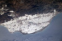
  Greenhouses in Almería as seen from space

Adoption

Worldwide, there are an estimated nine million acres of greenhouses.

Netherlands

Greenhouses in the Westland region.

The Netherlands has some of the largest greenhouses in the world. Such is the scale of food production in the country that in 2017, greenhouses occupied nearly 5,000 hectares.

Greenhouses began to be built in the Westland region of the Netherlands in the mid-19th century. The addition of sand to bogs and clay soil created fertile soil for agriculture, and around 1850, grapes were grown in the first greenhouses, simple glass constructions with one of the sides consisting of a solid wall. By the early 20th century, greenhouses began to be constructed with all sides built using glass, and they began to be heated. This also allowed for the production of fruits and vegetables that did not ordinarily grow in the area. Today, the Westland and the area around Aalsmeer have the highest concentration of greenhouse agriculture in the world. The Westland produces mostly vegetables, besides plants and flowers; Aalsmeer is noted mainly for the production of flowers and potted plants. Since the 20th century, the area around Venlo and parts of Drenthe have also become important regions for greenhouse agriculture.

Since 2000, technical innovations include the "closed greenhouse", a completely closed system allowing the grower complete control over the growing process while using less energy. Floating greenhouses are used in watery areas of the country.

The Netherlands has around 4,000 greenhouse enterprises that operate over 9,000 hectares of greenhouses and employ some 150,000 workers, producing €7.2 billion worth of vegetables, fruit, plants, and flowers, some 80% of which is exported.

Popper's experiment

From Wikipedia, the free encyclopedia
https://en.wikipedia.org/wiki/Popper%27s_experiment

Popper's experiment is an experiment proposed by the philosopher Karl Popper to put to the test different interpretations of quantum mechanics (QM). In fact, as early as 1934, Popper started criticising the increasingly more accepted Copenhagen interpretation, a popular subjectivist interpretation of quantum mechanics. Therefore, in his most famous book Logik der Forschung he proposed a first experiment alleged to empirically discriminate between the Copenhagen Interpretation and a realist interpretation, which he advocated. Einstein, however, wrote a letter to Popper about the experiment in which he raised some crucial objections and Popper himself declared that this first attempt was "a gross mistake for which I have been deeply sorry and ashamed of ever since".

Popper, however, came back to the foundations of quantum mechanics from 1948, when he developed his criticism of determinism in both quantum and classical physics. As a matter of fact, Popper greatly intensified his research activities on the foundations of quantum mechanics throughout the 1950s and 1960s developing his interpretation of quantum mechanics in terms of real existing probabilities (propensities), also thanks to the support of a number of distinguished physicists (such as David Bohm).

Overview

In 1980, Popper proposed perhaps his more important, yet overlooked, contribution to QM: a "new simplified version of the EPR experiment".

The experiment was however published only two years later, in the third volume of the Postscript to the Logic of Scientific Discovery.

The most widely known interpretation of quantum mechanics is the Copenhagen interpretation put forward by Niels Bohr and his school. It maintains that observations lead to a wavefunction collapse, thereby suggesting the counter-intuitive result that two well separated, non-interacting systems require action-at-a-distance. Popper argued that such non-locality conflicts with common sense, and would lead to a subjectivist interpretation of phenomena, depending on the role of the 'observer'.

While the EPR argument was always meant to be a thought experiment, put forward to shed light on the intrinsic paradoxes of QM, Popper proposed an experiment which could have been experimentally implemented and participated at a physics conference organised in Bari in 1983, to present his experiment and propose to the experimentalists to carry it out.

The actual realisation of Popper's experiment required new techniques which would make use of the phenomenon of spontaneous parametric down-conversion but had not yet been exploited at that time, so his experiment was eventually performed only in 1999, five years after Popper had died.

Description

Contrarily to the first (mistaken) proposal of 1934, Popper's experiment of 1980 exploits couples of entangled particles, in order to put to the test Heisenberg's uncertainty principle.

Indeed, Popper maintains:

"I wish to suggest a crucial experiment to test whether knowledge alone is sufficient to create 'uncertainty' and, with it, scatter (as is contended under the Copenhagen interpretation), or whether it is the physical situation that is responsible for the scatter."

Popper's proposed experiment consists of a low-intensity source of particles that can generate pairs of particles traveling to the left and to the right along the x-axis. The beam's low intensity is "so that the probability is high that two particles recorded at the same time on the left and on the right are those which have actually interacted before emission."

There are two slits, one each in the paths of the two particles. Behind the slits are semicircular arrays of counters which can detect the particles after they pass through the slits (see Fig. 1). "These counters are coincident counters [so] that they only detect particles that have passed at the same time through A and B."

Fig.1 Experiment with both slits equally wide. Both the particles should show equal scatter in their momenta.

Popper argued that because the slits localize the particles to a narrow region along the y-axis, from the uncertainty principle they experience large uncertainties in the y-components of their momenta. This larger spread in the momentum will show up as particles being detected even at positions that lie outside the regions where particles would normally reach based on their initial momentum spread.

Popper suggests that we count the particles in coincidence, i.e., we count only those particles behind slit B, whose partner has gone through slit A. Particles which are not able to pass through slit A are ignored.

The Heisenberg scatter for both the beams of particles going to the right and to the left, is tested "by making the two slits A and B wider or narrower. If the slits are narrower, then counters should come into play which are higher up and lower down, seen from the slits. The coming into play of these counters is indicative of the wider scattering angles which go with a narrower slit, according to the Heisenberg relations."

Fig.2 Experiment with slit A narrowed, and slit B wide open. Should the two particle show equal scatter in their momenta? If they do not, Popper says, the Copenhagen interpretation is wrong. If they do, it indicates action at a distance, says Popper.

Now the slit at A is made very small and the slit at B very wide. Popper wrote that, according to the EPR argument, we have measured position "y" for both particles (the one passing through A and the one passing through B) with the precision ${\displaystyle \Delta y}$, and not just for particle passing through slit A. This is because from the initial entangled EPR state we can calculate the position of the particle 2, once the position of particle 1 is known, with approximately the same precision. We can do this, argues Popper, even though slit B is wide open.

Therefore, Popper states that "fairly precise "knowledge"" about the y position of particle 2 is made; its y position is measured indirectly. And since it is, according to the Copenhagen interpretation, our knowledge which is described by the theory – and especially by the Heisenberg relations — it should be expected that the momentum ${\displaystyle p_{y}}$ of particle 2 scatters as much as that of particle 1, even though the slit A is much narrower than the widely opened slit at B.

Now the scatter can, in principle, be tested with the help of the counters. If the Copenhagen interpretation is correct, then such counters on the far side of B that are indicative of a wide scatter (and of a narrow slit) should now count coincidences: counters that did not count any particles before the slit A was narrowed.

To sum up: if the Copenhagen interpretation is correct, then any increase in the precision in the measurement of our mere knowledge of the particles going through slit B should increase their scatter.

Popper was inclined to believe that the test would decide against the Copenhagen interpretation, as it is applied to Heisenberg's uncertainty principle. If the test decided in favor of the Copenhagen interpretation, Popper argued, it could be interpreted as indicative of action at a distance.

The debate

Many viewed Popper's experiment as a crucial test of quantum mechanics, and there was a debate on what result an actual realization of the experiment would yield.

In 1985, Sudbery pointed out that the EPR state, which could be written as ${\displaystyle \psi (y_{1},y_{2})=\int _{-\infty }^{\infty }e^{iky_{1}}e^{-iky_{2}}\,dk}$, already contained an infinite spread in momenta (tacit in the integral over k), so no further spread could be seen by localizing one particle. Although it pointed to a crucial flaw in Popper's argument, its full implication was not understood. Kripps theoretically analyzed Popper's experiment and predicted that narrowing slit A would lead to momentum spread increasing at slit B. Kripps also argued that his result was based just on the formalism of quantum mechanics, without any interpretational problem. Thus, if Popper was challenging anything, he was challenging the central formalism of quantum mechanics.

In 1987 there came a major objection to Popper's proposal from Collet and Loudon. They pointed out that because the particle pairs originating from the source had a zero total momentum, the source could not have a sharply defined position. They showed that once the uncertainty in the position of the source is taken into account, the blurring introduced washes out the Popper effect.

Furthermore, Redhead analyzed Popper's experiment with a broad source and concluded that it could not yield the effect that Popper was seeking.

Realizations

Fig.3 Schematic diagram of Kim and Shih's experiment based on a BBO crystal which generates entangled photons. The lens LS helps create a sharp image of slit A on the location of slit B.

 

Fig.4 Results of the photon experiment by Kim and Shih, aimed at realizing Popper's proposal. The diffraction pattern in the absence of slit B (red symbols) is much narrower than that in the presence of a real slit (blue symbols).

Kim–Shih's experiment

Popper's experiment was realized in 1999 by Yoon-Ho Kim & Yanhua Shih using a spontaneous parametric down-conversion photon source. They did not observe an extra spread in the momentum of particle 2 due to particle 1 passing through a narrow slit. They write:

"Indeed, it is astonishing to see that the experimental results agree with Popper’s prediction. Through quantum entanglement one may learn the precise knowledge of a photon’s position and would therefore expect a greater uncertainty in its momentum under the usual Copenhagen interpretation of the uncertainty relations. However, the measurement shows that the momentum does not experience a corresponding increase in uncertainty. Is this a violation of the uncertainty principle?"

Rather, the momentum spread of particle 2 (observed in coincidence with particle 1 passing through slit A) was narrower than its momentum spread in the initial state.

They concluded that:

"Popper and EPR were correct in the prediction of the physical outcomes of their experiments. However, Popper and EPR made the same error by applying the results of two-particle physics to the explanation of the behavior of an individual particle. The two-particle entangled state is not the state of two individual particles. Our experimental result is emphatically NOT a violation of the uncertainty principle which governs the behavior of an individual quantum."

This led to a renewed heated debate, with some even going to the extent of claiming that Kim and Shih's experiment had demonstrated that there is no non-locality in quantum mechanics.

Unnikrishnan (2001), discussing Kim and Shih's result, wrote that the result:

"is a solid proof that there is no state-reduction-at-a-distance. ... Popper's experiment and its analysis forces us to radically change the current held view on quantum non-locality."

Short criticized Kim and Shih's experiment, arguing that because of the finite size of the source, the localization of particle 2 is imperfect, which leads to a smaller momentum spread than expected. However, Short's argument implies that if the source were improved, we should see a spread in the momentum of particle 2.

Sancho carried out a theoretical analysis of Popper's experiment, using the path-integral approach, and found a similar kind of narrowing in the momentum spread of particle 2, as was observed by Kim and Shih. Although this calculation did not give them any deep insight, it indicated that the experimental result of Kim-Shih agreed with quantum mechanics. It did not say anything about what bearing it has on the Copenhagen interpretation, if any.

Ghost diffraction

Popper's conjecture has also been tested experimentally in the so-called two-particle ghost interference experiment. This experiment was not carried out with the purpose of testing Popper's ideas, but ended up giving a conclusive result about Popper's test. In this experiment two entangled photons travel in different directions. Photon 1 goes through a slit, but there is no slit in the path of photon 2. However, Photon 2, if detected in coincidence with a fixed detector behind the slit detecting photon 1, shows a diffraction pattern. The width of the diffraction pattern for photon 2 increases when the slit in the path of photon 1 is narrowed. Thus, increase in the precision of knowledge about photon 2, by detecting photon 1 behind the slit, leads to increase in the scatter of photons 2.

Predictions according to quantum mechanics

Tabish Qureshi has published the following analysis of Popper's argument.

The ideal EPR state is written as ${\displaystyle |\psi \rangle =\int _{-\infty }^{\infty }|y,y\rangle \,dy=\int _{-\infty }^{\infty }|p,-p\rangle \,dp}$, where the two labels in the "ket" state represent the positions or momenta of the two particle. This implies perfect correlation, meaning, detecting particle 1 at position ${\displaystyle x_{0}}$ will also lead to particle 2 being detected at ${\displaystyle x_{0}}$. If particle 1 is measured to have a momentum ${\displaystyle p_{0}}$, particle 2 will be detected to have a momentum ${\displaystyle -p_{0}}$. The particles in this state have infinite momentum spread, and are infinitely delocalized. However, in the real world, correlations are always imperfect. Consider the following entangled state

${\displaystyle \psi (y_{1},y_{2})=A\!\int _{-\infty }^{\infty }dpe^{-{\frac {1}{4}}p^{2}\sigma ^{2}}e^{-{\frac {i}{\hbar }}py_{2}}e^{{\frac {i}{\hbar }}py_{1}}\exp \left[-{\frac {\left(y_{1}+y_{2}\right)^{2}}{16\Omega ^{2}}}\right]}$

where ${\displaystyle \sigma }$ represents a finite momentum spread, and ${\displaystyle \Omega }$ is a measure of the position spread of the particles. The uncertainties in position and momentum, for the two particles can be written as

${\displaystyle \Delta p_{2}=\Delta p_{1}={\sqrt {\sigma ^{2}+{\frac {\hbar ^{2}}{16\Omega ^{2}}}}},\qquad \Delta y_{1}=\Delta y_{2}={\sqrt {\Omega ^{2}+{\frac {\hbar ^{2}}{16\sigma ^{2}}}}}.}$

The action of a narrow slit on particle 1 can be thought of as reducing it to a narrow Gaussian state:

${\displaystyle \phi _{1}(y_{1})={\frac {1}{\left(2\pi \epsilon ^{2}\right)^{\frac {1}{4}}}}e^{-{\frac {y_{1}^{2}}{4\epsilon ^{2}}}}}$.

This will reduce the state of particle 2 to

${\displaystyle \phi _{2}(y_{2})=\!\int _{-\infty }^{\infty }\psi (y_{1},y_{2})\phi _{1}^{*}(y_{1})dy_{1}}$.

The momentum uncertainty of particle 2 can now be calculated, and is given by

${\displaystyle \Delta p_{2}={\sqrt {\frac {\sigma ^{2}\left(1+{\frac {\epsilon ^{2}}{\Omega ^{2}}}\right)+{\frac {\hbar ^{2}}{16\Omega ^{2}}}}{1+4\epsilon ^{2}\left({\frac {\sigma ^{2}}{\hbar ^{2}}}+{\frac {1}{16\Omega ^{2}}}\right)}}}.}$

If we go to the extreme limit of slit A being infinitesimally narrow (${\displaystyle \epsilon \to 0}$), the momentum uncertainty of particle 2 is ${\textstyle \lim _{\epsilon \to 0}\Delta p_{2}={\sqrt {\sigma ^{2}+\hbar ^{2}/16\Omega ^{2}}}}$, which is exactly what the momentum spread was to begin with. In fact, one can show that the momentum spread of particle 2, conditioned on particle 1 going through slit A, is always less than or equal to ${\textstyle {\sqrt {\sigma ^{2}+\hbar ^{2}/16\Omega ^{2}}}}$ (the initial spread), for any value of ${\displaystyle \epsilon ,\sigma }$, and ${\displaystyle \Omega }$. Thus, particle 2 does not acquire any extra momentum spread than it already had. This is the prediction of standard quantum mechanics. So, the momentum spread of particle 2 will always be smaller than what was contained in the original beam. This is what was actually seen in the experiment of Kim and Shih. Popper's proposed experiment, if carried out in this way, is incapable of testing the Copenhagen interpretation of quantum mechanics.

On the other hand, if slit A is gradually narrowed, the momentum spread of particle 2 (conditioned on the detection of particle 1 behind slit A) will show a gradual increase (never beyond the initial spread, of course). This is what quantum mechanics predicts. Popper had said

"...if the Copenhagen interpretation is correct, then any increase in the precision in the measurement of our mere knowledge of the particles going through slit B should increase their scatter."

This particular aspect can be experimentally tested.

Faster-than-light signalling

The expected additional momentum scatter which Popper wrongly attributed to the Copenhagen interpretation would allow faster-than-light communication, which is excluded by the no-communication theorem in quantum mechanics. Note however that both Collet and Loudon and Qureshi compute that scatter decreases with decreasing the size of slit A, contrary to the increase predicted by Popper. There was some controversy about this decrease also allowing superluminal communication. But the reduction is of the standard deviation of the conditional distribution of the position of particle 2 knowing that particle 1 did go through slit A, since we are only counting coincident detection. The reduction in conditional distribution allows for the unconditional distribution to remain the same, which is the only thing that matters to exclude superluminal communication. Also note that the conditional distribution would be different from the unconditional distribution in classical physics as well. But measuring the conditional distribution after slit B requires the information on the result at slit A, which has to be communicated classically, so that the conditional distribution cannot be known as soon as the measurement is made at slit A but is delayed by the time required to transmit that information.

Protein structure

From Wikipedia, the free encyclopedia

https://en.wikipedia.org/wiki/Protein_structure 

 

Interactive diagram of protein structure, using PCNA as an example. (PDB: 1AXC​)

Protein structure is the three-dimensional arrangement of atoms in an amino acid-chain molecule. Proteins are polymers – specifically polypeptides – formed from sequences of amino acids, the monomers of the polymer. A single amino acid monomer may also be called a residue indicating a repeating unit of a polymer. Proteins form by amino acids undergoing condensation reactions, in which the amino acids lose one water molecule per reaction in order to attach to one another with a peptide bond. By convention, a chain under 30 amino acids is often identified as a peptide, rather than a protein. To be able to perform their biological function, proteins fold into one or more specific spatial conformations driven by a number of non-covalent interactions such as hydrogen bonding, ionic interactions, Van der Waals forces, and hydrophobic packing. To understand the functions of proteins at a molecular level, it is often necessary to determine their three-dimensional structure. This is the topic of the scientific field of structural biology, which employs techniques such as X-ray crystallography, NMR spectroscopy, cryo electron microscopy (cryo-EM) and dual polarisation interferometry to determine the structure of proteins.

Protein structures range in size from tens to several thousand amino acids. By physical size, proteins are classified as nanoparticles, between 1–100 nm. Very large protein complexes can be formed from protein subunits. For example, many thousands of actin molecules assemble into a microfilament.

A protein usually undergoes reversible structural changes in performing its biological function. The alternative structures of the same protein are referred to as different conformations, and transitions between them are called conformational changes.

Levels of protein structure

There are four distinct levels of protein structure.

Four levels of protein structure

Primary structure

Main article: Protein primary structure

The primary structure of a protein refers to the sequence of amino acids in the polypeptide chain. The primary structure is held together by peptide bonds that are made during the process of protein biosynthesis. The two ends of the polypeptide chain are referred to as the carboxyl terminus (C-terminus) and the amino terminus (N-terminus) based on the nature of the free group on each extremity. Counting of residues always starts at the N-terminal end (NH₂-group), which is the end where the amino group is not involved in a peptide bond. The primary structure of a protein is determined by the gene corresponding to the protein. A specific sequence of nucleotides in DNA is transcribed into mRNA, which is read by the ribosome in a process called translation. The sequence of amino acids in insulin was discovered by Frederick Sanger, establishing that proteins have defining amino acid sequences. The sequence of a protein is unique to that protein, and defines the structure and function of the protein. The sequence of a protein can be determined by methods such as Edman degradation or tandem mass spectrometry. Often, however, it is read directly from the sequence of the gene using the genetic code. It is strictly recommended to use the words "amino acid residues" when discussing proteins because when a peptide bond is formed, a water molecule is lost, and therefore proteins are made up of amino acid residues. Post-translational modifications such as phosphorylations and glycosylations are usually also considered a part of the primary structure, and cannot be read from the gene. For example, insulin is composed of 51 amino acids in 2 chains. One chain has 31 amino acids, and the other has 20 amino acids.

Secondary structure

An α-helix with hydrogen bonds (yellow dots)

 

Main article: Protein secondary structure

Secondary structure refers to highly regular local sub-structures on the actual polypeptide backbone chain. Two main types of secondary structure, the α-helix and the β-strand or β-sheets, were suggested in 1951 by Linus Pauling et al. These secondary structures are defined by patterns of hydrogen bonds between the main-chain peptide groups. They have a regular geometry, being constrained to specific values of the dihedral angles ψ and φ on the Ramachandran plot. Both the α-helix and the β-sheet represent a way of saturating all the hydrogen bond donors and acceptors in the peptide backbone. Some parts of the protein are ordered but do not form any regular structures. They should not be confused with random coil, an unfolded polypeptide chain lacking any fixed three-dimensional structure. Several sequential secondary structures may form a "supersecondary unit".

Tertiary structure

Main article: Protein tertiary structure

Tertiary structure refers to the three-dimensional structure created by a single protein molecule (a single polypeptide chain). It may include one or several domains. The α-helixes and β-pleated-sheets are folded into a compact globular structure. The folding is driven by the non-specific hydrophobic interactions, the burial of hydrophobic residues from water, but the structure is stable only when the parts of a protein domain are locked into place by specific tertiary interactions, such as salt bridges, hydrogen bonds, and the tight packing of side chains and disulfide bonds. The disulfide bonds are extremely rare in cytosolic proteins, since the cytosol (intracellular fluid) is generally a reducing environment.

Quaternary structure

Main article: Protein quaternary structure

Quaternary structure is the three-dimensional structure consisting of the aggregation of two or more individual polypeptide chains (subunits) that operate as a single functional unit (multimer). The resulting multimer is stabilized by the same non-covalent interactions and disulfide bonds as in tertiary structure. There are many possible quaternary structure organisations. Complexes of two or more polypeptides (i.e. multiple subunits) are called multimers. Specifically it would be called a dimer if it contains two subunits, a trimer if it contains three subunits, a tetramer if it contains four subunits, and a pentamer if it contains five subunits. The subunits are frequently related to one another by symmetry operations, such as a 2-fold axis in a dimer. Multimers made up of identical subunits are referred to with a prefix of "homo-" and those made up of different subunits are referred to with a prefix of "hetero-", for example, a heterotetramer, such as the two alpha and two beta chains of hemoglobin.

Domains, motifs, and folds in protein structure

Protein domains. The two shown protein structures share a common domain (maroon), the PH domain, which is involved in phosphatidylinositol (3,4,5)-trisphosphate binding

Proteins are frequently described as consisting of several structural units. These units include domains, motifs, and folds. Despite the fact that there are about 100,000 different proteins expressed in eukaryotic systems, there are many fewer different domains, structural motifs and folds.

Structural domain

A structural domain is an element of the protein's overall structure that is self-stabilizing and often folds independently of the rest of the protein chain. Many domains are not unique to the protein products of one gene or one gene family but instead appear in a variety of proteins. Domains often are named and singled out because they figure prominently in the biological function of the protein they belong to; for example, the "calcium-binding domain of calmodulin". Because they are independently stable, domains can be "swapped" by genetic engineering between one protein and another to make chimera proteins. A conservative combination of several domains that occur in different proteins, such as protein tyrosine phosphatase domain and C2 domain pair, was called "a superdomain" that may evolve as a single unit.

Structural and sequence motifs

The structural and sequence motifs refer to short segments of protein three-dimensional structure or amino acid sequence that were found in a large number of different proteins

Supersecondary structure

Tertiary protein structures can have multiple secondary elements on the same polypeptide chain. The supersecondary structure refers to a specific combination of secondary structure elements, such as β-α-β units or a helix-turn-helix motif. Some of them may be also referred to as structural motifs.

Protein fold

A protein fold refers to the general protein architecture, like a helix bundle, β-barrel, Rossmann fold or different "folds" provided in the Structural Classification of Proteins database. A related concept is protein topology.

Protein dynamics and conformational ensembles

Main article: Protein dynamics

Proteins are not static objects, but rather populate ensembles of conformational states. Transitions between these states typically occur on nanoscales, and have been linked to functionally relevant phenomena such as allosteric signaling and enzyme catalysis. Protein dynamics and conformational changes allow proteins to function as nanoscale biological machines within cells, often in the form of multi-protein complexes. Examples include motor proteins, such as myosin, which is responsible for muscle contraction, kinesin, which moves cargo inside cells away from the nucleus along microtubules, and dynein, which moves cargo inside cells towards the nucleus and produces the axonemal beating of motile cilia and flagella. "[I]n effect, the [motile cilium] is a nanomachine composed of perhaps over 600 proteins in molecular complexes, many of which also function independently as nanomachines...Flexible linkers allow the mobile protein domains connected by them to recruit their binding partners and induce long-range allostery via protein domain dynamics. "

Schematic view of the two main ensemble modeling approaches.

Proteins are often thought of as relatively stable tertiary structures that experience conformational changes after being affected by interactions with other proteins or as a part of enzymatic activity. However, proteins may have varying degrees of stability, and some of the less stable variants are intrinsically disordered proteins. These proteins exist and function in a relatively 'disordered' state lacking a stable tertiary structure. As a result, they are difficult to describe by a single fixed tertiary structure. Conformational ensembles have been devised as a way to provide a more accurate and 'dynamic' representation of the conformational state of intrinsically disordered proteins.

Protein ensemble files are a representation of a protein that can be considered to have a flexible structure. Creating these files requires determining which of the various theoretically possible protein conformations actually exist. One approach is to apply computational algorithms to the protein data in order to try to determine the most likely set of conformations for an ensemble file. There are multiple methods for preparing data for the Protein Ensemble Database that fall into two general methodologies – pool and molecular dynamics (MD) approaches (diagrammed in the figure). The pool based approach uses the protein’s amino acid sequence to create a massive pool of random conformations. This pool is then subjected to more computational processing that creates a set of theoretical parameters for each conformation based on the structure. Conformational subsets from this pool whose average theoretical parameters closely match known experimental data for this protein are selected. The alternative molecular dynamics approach takes multiple random conformations at a time and subjects all of them to experimental data. Here the experimental data is serving as limitations to be placed on the conformations (e.g. known distances between atoms). Only conformations that manage to remain within the limits set by the experimental data are accepted. This approach often applies large amounts of experimental data to the conformations which is a very computationally demanding task.

The conformational ensembles were generated for a number of highly dynamic and partially unfolded proteins, such as Sic1/Cdc4, p15 PAF, MKK7, Beta-synuclein and P27.

Protein folding

Main article: Protein folding

As it is translated, polypeptides exit the ribosome mostly as a random coil and folds into its native state. The final structure of the protein chain is generally assumed to be determined by its amino acid sequence (Anfinsen's dogma).

Protein stability

Main article: Equilibrium unfolding

Thermodynamic stability of proteins represents the free energy difference between the folded and unfolded protein states. This free energy difference is very sensitive to temperature, hence a change in temperature may result in unfolding or denaturation. Protein denaturation may result in loss of function, and loss of native state. The free energy of stabilization of soluble globular proteins typically does not exceed 50 kJ/mol. Taking into consideration the large number of hydrogen bonds that take place for the stabilization of secondary structures, and the stabilization of the inner core through hydrophobic interactions, the free energy of stabilization emerges as small difference between large numbers.

Protein structure determination

Examples of protein structures from the PDB

 

Rate of Protein Structure Determination by Method and Year

Around 90% of the protein structures available in the Protein Data Bank have been determined by X-ray crystallography. This method allows one to measure the three-dimensional (3-D) density distribution of electrons in the protein, in the crystallized state, and thereby infer the 3-D coordinates of all the atoms to be determined to a certain resolution. Roughly 9% of the known protein structures have been obtained by nuclear magnetic resonance (NMR) techniques. For larger protein complexes, cryo-electron microscopy can determine protein structures. The resolution is typically lower than that of X-ray crystallography, or NMR, but the maximum resolution is steadily increasing. This technique is still a particularly valuable for very large protein complexes such as virus coat proteins and amyloid fibers.

General secondary structure composition can be determined via circular dichroism. Vibrational spectroscopy can also be used to characterize the conformation of peptides, polypeptides, and proteins. Two-dimensional infrared spectroscopy has become a valuable method to investigate the structures of flexible peptides and proteins that cannot be studied with other methods. A more qualitative picture of protein structure is often obtained by proteolysis, which is also useful to screen for more crystallizable protein samples. Novel implementations of this approach, including fast parallel proteolysis (FASTpp), can probe the structured fraction and its stability without the need for purification. Once a protein's structure has been experimentally determined, further detailed studies can be done computationally, using molecular dynamic simulations of that structure.

Protein structure databases

A protein structure database is a database that is modeled around the various experimentally determined protein structures. The aim of most protein structure databases is to organize and annotate the protein structures, providing the biological community access to the experimental data in a useful way. Data included in protein structure databases often includes 3D coordinates as well as experimental information, such as unit cell dimensions and angles for x-ray crystallography determined structures. Though most instances, in this case either proteins or a specific structure determinations of a protein, also contain sequence information and some databases even provide means for performing sequence based queries, the primary attribute of a structure database is structural information, whereas sequence databases focus on sequence information, and contain no structural information for the majority of entries. Protein structure databases are critical for many efforts in computational biology such as structure based drug design, both in developing the computational methods used and in providing a large experimental dataset used by some methods to provide insights about the function of a protein.

Structural classifications of proteins

Protein structures can be grouped based on their structural similarity, topological class or a common evolutionary origin. The Structural Classification of Proteins database and CATH database provide two different structural classifications of proteins. When the structural similarity is large the two proteins have possibly diverged from a common ancestor, and shared structure between proteins is considered evidence of homology. Structure similarity can then be used to group proteins together into protein superfamilies. If shared structure is significant but the fraction shared is small, the fragment shared may be the consequence of a more dramatic evolutionary event such as horizontal gene transfer, and joining proteins sharing these fragments into protein superfamilies is no longer justified. Topology of a protein can be used to classify proteins as well. Knot theory and circuit topology are two topology frameworks developed for classification of protein folds based on chain crossing and intrachain contacts respectively.

Computational prediction of protein structure

Main article: Protein structure prediction

The generation of a protein sequence is much easier than the determination of a protein structure. However, the structure of a protein gives much more insight in the function of the protein than its sequence. Therefore, a number of methods for the computational prediction of protein structure from its sequence have been developed. Ab initio prediction methods use just the sequence of the protein. Threading and homology modeling methods can build a 3-D model for a protein of unknown structure from experimental structures of evolutionarily-related proteins, called a protein family.