Linear algebra

From Wikipedia, the free encyclopedia

The three-dimensional Euclidean space R³ is a vector space, and lines and planes passing through the origin are vector subspaces in R³.

Linear algebra is the branch of mathematics concerning vector spaces and linear mappings between such spaces. It includes the study of lines, planes, and subspaces, but is also concerned with properties common to all vector spaces.

The set of points with coordinates that satisfy a linear equation form a hyperplane in an n-dimensional space. The conditions under which a set of n hyperplanes intersect in a single point is an important focus of study in linear algebra. Such an investigation is initially motivated by a system of linear equations containing several unknowns. Such equations are naturally represented using the formalism of matrices and vectors.^[1][2]

Linear algebra is central to both pure and applied mathematics. For instance, abstract algebra arises by relaxing the axioms of a vector space, leading to a number of generalizations. Functional analysis studies the infinite-dimensional version of the theory of vector spaces. Combined with calculus, linear algebra facilitates the solution of linear systems of differential equations.

Techniques from linear algebra are also used in analytic geometry, engineering, physics, natural sciences, computer science, computer animation, and the social sciences (particularly in economics). Because linear algebra is such a well-developed theory, nonlinear mathematical models are sometimes approximated by linear models.

History

The study of linear algebra first emerged from the study of determinants, which were used to solve systems of linear equations. Determinants were used by Leibniz in 1693, and subsequently, Gabriel Cramer devised Cramer's Rule for solving linear systems in 1750. Later, Gauss further developed the theory of solving linear systems by using Gaussian elimination, which was initially listed as an advancement in geodesy.^[3]

The study of matrix algebra first emerged in England in the mid-1800s. In 1844 Hermann Grassmann published his “Theory of Extension” which included foundational new topics of what is today called linear algebra. In 1848, James Joseph Sylvester introduced the term matrix, which is Latin for "womb". While studying compositions of linear transformations, Arthur Cayley was led to define matrix multiplication and inverses. Crucially, Cayley used a single letter to denote a matrix, thus treating a matrix as an aggregate object. He also realized the connection between matrices and determinants, and wrote "There would be many things to say about this theory of matrices which should, it seems to me, precede the theory of determinants".^[3]

In 1882, Hüseyin Tevfik Pasha wrote the book titled "Linear Algebra".^[4][5] The first modern and more precise definition of a vector space was introduced by Peano in 1888;^[3] by 1900, a theory of linear transformations of finite-dimensional vector spaces had emerged. Linear algebra first took its modern form in the first half of the twentieth century, when many ideas and methods of previous centuries were generalized as abstract algebra. The use of matrices in quantum mechanics, special relativity, and statistics helped spread the subject of linear algebra beyond pure mathematics. The development of computers led to increased research in efficient algorithms for Gaussian elimination and matrix decompositions, and linear algebra became an essential tool for modelling and simulations.^[3]

The origin of many of these ideas is discussed in the articles on determinants and Gaussian elimination.

Educational history

Linear algebra first appeared in graduate textbooks in the 1940s and in undergraduate textbooks in the 1950s.^[6] Following work by the School Mathematics Study Group, U.S. high schools asked 12th grade students to do "matrix algebra, formerly reserved for college" in the 1960s.^[7] In France during the 1960s, educators attempted to teach linear algebra through affine dimensional vector spaces in the first year of secondary school. This was met with a backlash in the 1980s that removed linear algebra from the curriculum.^[8] In 1993, the U.S.-based Linear Algebra Curriculum Study Group recommended that undergraduate linear algebra courses be given an application-based "matrix orientation" as opposed to a theoretical orientation.^[9]

Scope of study

Vector spaces

The main structures of linear algebra are vector spaces. A vector space over a field F is a set V together with two binary operations. Elements of V are called vectors and elements of F are called scalars. The first operation, vector addition, takes any two vectors v and w and outputs a third vector v + w. The second operation, scalar multiplication, takes any scalar a and any vector v and outputs a new vector av. The operations of addition and multiplication in a vector space must satisfy the following axioms.^[10] In the list below, let u, v and w be arbitrary vectors in V, and a and b scalars in F.

Axiom	Signification
Associativity of addition	u + (v + w) = (u + v) + w
Commutativity of addition	u + v = v + u
Identity element of addition	There exists an element 0 ∈ V, called the zero vector, such that v + 0 = v for all v ∈ V.
Inverse elements of addition	For every v ∈ V, there exists an element −v ∈ V, called the additive inverse of v, such that v + (−v) = 0
Distributivity of scalar multiplication with respect to vector addition	a(u + v) = au + av
Distributivity of scalar multiplication with respect to field addition	(a + b)v = av + bv
Compatibility of scalar multiplication with field multiplication	a(bv) = (ab)v [nb 1]
Identity element of scalar multiplication	1v = v, where 1 denotes the multiplicative identity in F.

The first four axioms are those of V being an abelian group under vector addition. Vector spaces may be diverse in nature, for example, containing functions, polynomials or matrices. Linear algebra is concerned with properties common to all vector spaces.

Linear transformations

Similarly as in the theory of other algebraic structures, linear algebra studies mappings between vector spaces that preserve the vector-space structure. Given two vector spaces V and W over a field F, a linear transformation (also called linear map, linear mapping or linear operator) is a map

that is compatible with addition and scalar multiplication:

for any vectors u,v ∈ V and a scalar a ∈ F.

Additionally for any vectors u, v ∈ V and scalars a, b ∈ F:

When a bijective linear mapping exists between two vector spaces (that is, every vector from the second space is associated with exactly one in the first), we say that the two spaces are isomorphic. Because an isomorphism preserves linear structure, two isomorphic vector spaces are "essentially the same" from the linear algebra point of view. One essential question in linear algebra is whether a mapping is an isomorphism or not, and this question can be answered by checking if the determinant is nonzero. If a mapping is not an isomorphism, linear algebra is interested in finding its range (or image) and the set of elements that get mapped to zero, called the kernel of the mapping.

Linear transformations have geometric significance. For example, 2 × 2 real matrices denote standard planar mappings that preserve the origin.

Subspaces, span, and basis

Again, in analogue with theories of other algebraic objects, linear algebra is interested in subsets of vector spaces that are themselves vector spaces; these subsets are called linear subspaces. For example, both the range and kernel of a linear mapping are subspaces, and are thus often called the range space and the nullspace; these are important examples of subspaces. Another important way of forming a subspace is to take a linear combination of a set of vectors v₁, v₂, …, v_k:

where a₁, a₂, …, a_k are scalars. The set of all linear combinations of vectors v₁, v₂, …, v_k is called their span, which forms a subspace.

A linear combination of any system of vectors with all zero coefficients is the zero vector of V. If this is the only way to express the zero vector as a linear combination of v₁, v₂, …, v_k then these vectors are linearly independent. Given a set of vectors that span a space, if any vector w is a linear combination of other vectors (and so the set is not linearly independent), then the span would remain the same if we remove w from the set. Thus, a set of linearly dependent vectors is redundant in the sense that there will be a linearly independent subset which will span the same subspace. Therefore, we are mostly interested in a linearly independent set of vectors that spans a vector space V, which we call a basis of V. Any set of vectors that spans V contains a basis, and any linearly independent set of vectors in V can be extended to a basis.^[11] It turns out that if we accept the axiom of choice, every vector space has a basis;^[12] nevertheless, this basis may be unnatural, and indeed, may not even be constructible. For instance, there exists a basis for the real numbers considered as a vector space over the rationals, but no explicit basis has been constructed.

Any two bases of a vector space V have the same cardinality, which is called the dimension of V. The dimension of a vector space is well-defined by the dimension theorem for vector spaces. If a basis of V has finite number of elements, V is called a finite-dimensional vector space. If V is finite-dimensional and U is a subspace of V, then dim U ≤ dim V. If U₁ and U₂ are subspaces of V, then

.^[13]

One often restricts consideration to finite-dimensional vector spaces. A fundamental theorem of linear algebra states that all vector spaces of the same dimension are isomorphic,^[14] giving an easy way of characterizing isomorphism.

Matrix theory

A particular basis {v₁, v₂, …, v_n} of V allows one to construct a coordinate system in V: the vector with coordinates (a₁, a₂, …, a_n) is the linear combination

The condition that v₁, v₂, …, v_n span V guarantees that each vector v can be assigned coordinates, whereas the linear independence of v₁, v₂, …, v_n assures that these coordinates are unique (i.e. there is only one linear combination of the basis vectors that is equal to v). In this way, once a basis of a vector space V over F has been chosen, V may be identified with the coordinate n-space Fⁿ. Under this identification, addition and scalar multiplication of vectors in V correspond to addition and scalar multiplication of their coordinate vectors in Fⁿ. Furthermore, if V and W are an n-dimensional and m-dimensional vector space over F, and a basis of V and a basis of W have been fixed, then any linear transformation T: V → W may be encoded by an m × n matrix A with entries in the field F, called the matrix of T with respect to these bases. Two matrices that encode the same linear transformation in different bases are called similar. Matrix theory replaces the study of linear transformations, which were defined axiomatically, by the study of matrices, which are concrete objects. This major technique distinguishes linear algebra from theories of other algebraic structures, which usually cannot be parameterized so concretely.

There is an important distinction between the coordinate n-space Rⁿ and a general finite-dimensional vector space V. While Rⁿ has a standard basis {e₁, e₂, …, e_n}, a vector space V typically does not come equipped with such a basis and many different bases exist (although they all consist of the same number of elements equal to the dimension of V).

One major application of the matrix theory is calculation of determinants, a central concept in linear algebra. While determinants could be defined in a basis-free manner, they are usually introduced via a specific representation of the mapping; the value of the determinant does not depend on the specific basis. It turns out that a mapping has an inverse if and only if the determinant has an inverse (every non-zero real or complex number has an inverse^[15]). If the determinant is zero, then the nullspace is nontrivial. Determinants have other applications, including a systematic way of seeing if a set of vectors is linearly independent (we write the vectors as the columns of a matrix, and if the determinant of that matrix is zero, the vectors are linearly dependent). Determinants could also be used to solve systems of linear equations (see Cramer's rule), but in real applications, Gaussian elimination is a faster method.

Eigenvalues and eigenvectors

In general, the action of a linear transformation may be quite complex. Attention to low-dimensional examples gives an indication of the variety of their types. One strategy for a general n-dimensional transformation T is to find "characteristic lines" that are invariant sets under T. If v is a non-zero vector such that Tv is a scalar multiple of v, then the line through 0 and v is an invariant set under T and v is called a characteristic vector or eigenvector. The scalar λ such that Tv = λv is called a characteristic value or eigenvalue of T.

To find an eigenvector or an eigenvalue, we note that

where I is the identity matrix. For there to be nontrivial solutions to that equation, det(T − λ I) = 0. The determinant is a polynomial, and so the eigenvalues are not guaranteed to exist if the field is R. Thus, we often work with an algebraically closed field such as the complex numbers when dealing with eigenvectors and eigenvalues so that an eigenvalue will always exist. It would be particularly nice if given a transformation T taking a vector space V into itself we can find a basis for V consisting of eigenvectors. If such a basis exists, we can easily compute the action of the transformation on any vector: if v₁, v₂, …, v_n are linearly independent eigenvectors of a mapping of n-dimensional spaces T with (not necessarily distinct) eigenvalues λ₁, λ₂, …, λ_n, and if v = a₁v₁ + ... + a_n v_n, then,

Such a transformation is called a diagonalizable matrix since in the eigenbasis, the transformation is represented by a diagonal matrix. Because operations like matrix multiplication, matrix inversion, and determinant calculation are simple on diagonal matrices, computations involving matrices are much simpler if we can bring the matrix to a diagonal form. Not all matrices are diagonalizable (even over an algebraically closed field).

Inner-product spaces

Besides these basic concepts, linear algebra also studies vector spaces with additional structure, such as an inner product. The inner product is an example of a bilinear form, and it gives the vector space a geometric structure by allowing for the definition of length and angles. Formally, an inner product is a map

that satisfies the following three axioms for all vectors u, v, w in V and all scalars a in F:^[16][17]

• Conjugate symmetry:

Note that in R, it is symmetric.

• Linearity in the first argument:

• Positive-definiteness:

with equality only for v = 0.

We can define the length of a vector v in V by

and we can prove the Cauchy–Schwarz inequality:

In particular, the quantity

and so we can call this quantity the cosine of the angle between the two vectors.

Two vectors are orthogonal if . An orthonormal basis is a basis where all basis vectors have length 1 and are orthogonal to each other. Given any finite-dimensional vector space, an orthonormal basis could be found by the Gram–Schmidt procedure. Orthonormal bases are particularly nice to deal with, since if v = a₁ v₁ + ... + a_n v_n, then .

The inner product facilitates the construction of many useful concepts. For instance, given a transform T, we can define its Hermitian conjugate T* as the linear transform satisfying

If T satisfies TT* = T*T, we call T normal. It turns out that normal matrices are precisely the matrices that have an orthonormal system of eigenvectors that span V.

Some main useful theorems

• A matrix is invertible, or non-singular, if and only if the linear map represented by the matrix is an isomorphism.
• Any vector space over a field F of dimension n is isomorphic to Fⁿ as a vector space over F.
• Corollary: Any two vector spaces over F of the same finite dimension are isomorphic to each other.
• A linear map is an isomorphism if and only if the determinant is nonzero.

Applications

Because of the ubiquity of vector spaces, linear algebra is used in many fields of mathematics, natural sciences, computer science, and social science. Below are just some examples of applications of linear algebra.

Solution of linear systems

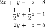
Linear algebra provides the formal setting for the linear combination of equations used in the Gaussian method. Suppose the goal is to find and describe the solution(s), if any, of the following system of linear equations:

The Gaussian-elimination algorithm is as follows: eliminate x from all equations below L₁, and then eliminate y from all equations below L₂. This will put the system into triangular form. Then, using back-substitution, each unknown can be solved for.

In the example, x is eliminated from L₂ by adding (3/2)L₁ to L₂. x is then eliminated from L₃ by adding L₁ to L₃. Formally:

The result is:

Now y is eliminated from L₃ by adding −4L₂ to L₃:

The result is:

This result is a system of linear equations in triangular form, and so the first part of the algorithm is complete.
The last part, back-substitution, consists of solving for the known in reverse order. It can thus be seen that

Then, z can be substituted into L₂, which can then be solved to obtain

Next, z and y can be substituted into L₁, which can be solved to obtain

The system is solved.

We can, in general, write any system of linear equations as a matrix equation:

The solution of this system is characterized as follows: first, we find a particular solution x₀ of this equation using Gaussian elimination. Then, we compute the solutions of Ax = 0; that is, we find the null space N of A. The solution set of this equation is given by . If the number of variables equal the number of equations, then we can characterize when the system has a unique solution: since N is trivial if and only if det A ≠ 0, the equation has a unique solution if and only if det A ≠ 0.^[18]

Least-squares best fit line

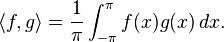
The least squares method is used to determine the best fit line for a set of data.^[19] This line will minimize the sum of the squares of the residuals.

Fourier series expansion

Fourier series are a representation of a function f: [−π, π] → R as a trigonometric series:

This series expansion is extremely useful in solving partial differential equations. In this article, we will not be concerned with convergence issues; it is nice to note that all Lipschitz-continuous functions have a converging Fourier series expansion, and nice enough discontinuous functions have a Fourier series that converges to the function value at most points.

The space of all functions that can be represented by a Fourier series form a vector space (technically speaking, we call functions that have the same Fourier series expansion the "same" function, since two different discontinuous functions might have the same Fourier series). Moreover, this space is also an inner product space with the inner product

The functions g_n(x) = sin(nx) for n > 0 and h_n(x) = cos(nx) for n ≥ 0 are an orthonormal basis for the space of Fourier-expandable functions. We can thus use the tools of linear algebra to find the expansion of any function in this space in terms of these basis functions. For instance, to find the coefficient a_k, we take the inner product with h_k:

and by orthonormality, ; that is,

Quantum mechanics

Quantum mechanics is highly inspired by notions in linear algebra. In quantum mechanics, the physical state of a particle is represented by a vector, and observables (such as momentum, energy, and angular momentum) are represented by linear operators on the underlying vector space. More concretely, the wave function of a particle describes its physical state and lies in the vector space L² (the functions φ: R³ → C such that is finite), and it evolves according to the Schrödinger equation. Energy is represented as the operator , where V is the potential energy. H is also known as the Hamiltonian operator. The eigenvalues of H represents the possible energies that can be observed. Given a particle in some state φ, we can expand φ into a linear combination of eigenstates of H. The component of H in each eigenstate determines the probability of measuring the corresponding eigenvalue, and the measurement forces the particle to assume that eigenstate (wave function collapse).

Geometric introduction

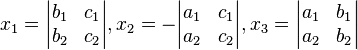
Many of the principles and techniques of linear algebra can be seen in the geometry of lines in a real two dimensional plane E. When formulated using vectors and matrices the geometry of points and lines in the plane can be extended to the geometry of points and hyperplanes in high-dimensional spaces.

Point coordinates in the plane E are ordered pairs of real numbers, (x,y), and a line is defined as the set of points (x,y) that satisfy the linear equation^[20]

,

where a, b and c are not all zero. Then,

or

where x = (x, y, 1) is the 3 × 1 set of homogeneous coordinates associated with the point (x, y).^[21]

Homogeneous coordinates identify the plane E with the z = 1 plane in three dimensional space. The x−y coordinates in E are obtained from homogeneous coordinates y = (y₁, y₂, y₃) by dividing by the third component (if it is nonzero) to obtain y = (y₁/y₃, y₂/y₃, 1).

The linear equation, λ, has the important property, that if x₁ and x₂ are homogeneous coordinates of points on the line, then the point αx₁ + βx₂ is also on the line, for any real α and β.

Now consider the equations of the two lines λ₁ and λ₂,

which forms a system of linear equations. The intersection of these two lines is defined by x = (x, y, 1) that satisfy the matrix equation,

or using homogeneous coordinates,

The point of intersection of these two lines is the unique non-zero solution of these equations. In homogeneous coordinates, the solutions are multiples of the following solution:^[21]

if the rows of B are linearly independent (i.e., λ₁ and λ₂ represent distinct lines). Divide through by x₃ to get Cramer's rule for the solution of a set of two linear equations in two unknowns.^[22] Notice that this yields a point in the z = 1 plane only when the 2 × 2 submatrix associated with x₃ has a non-zero determinant.

It is interesting to consider the case of three lines, λ₁, λ₂ and λ₃, which yield the matrix equation,

which in homogeneous form yields,

Clearly, this equation has the solution x = (0,0,0), which is not a point on the z = 1 plane E. For a solution to exist in the plane E, the coefficient matrix C must have rank 2, which means its determinant must be zero. Another way to say this is that the columns of the matrix must be linearly dependent.

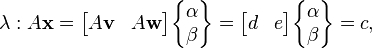
Introduction to linear transformations

Another way to approach linear algebra is to consider linear functions on the two dimensional real plane E=R². Here R denotes the set of real numbers. Let x=(x, y) be an arbitrary vector in E and consider the linear function λ: E→R, given by

or

This transformation has the important property that if Ay=d, then

This shows that the sum of vectors in E map to the sum of their images in R. This is the defining characteristic of a linear map, or linear transformation.^[20] For this case, where the image space is a real number the map is called a linear functional.^[22]

Consider the linear functional a little more carefully. Let i=(1,0) and j =(0,1) be the natural basis vectors on E, so that x=xi+yj. It is now possible to see that

Thus, the columns of the matrix A are the image of the basis vectors of E in R.

This is true for any pair of vectors used to define coordinates in E. Suppose we select a non-orthogonal non-unit vector basis v and w to define coordinates of vectors in E. This means a vector x has coordinates (α,β), such that x=αv+βw. Then, we have the linear functional

where Av=d and Aw=e are the images of the basis vectors v and w. This is written in matrix form as

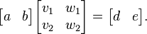
Coordinates relative to a basis

This leads to the question of how to determine the coordinates of a vector x relative to a general basis v and w in E. Assume that we know the coordinates of the vectors, x, v and w in the natural basis i=(1,0) and j =(0,1). Our goal is two find the real numbers α, β, so that x=αv+βw, that is

To solve this equation for α, β, we compute the linear coordinate functionals σ and τ for the basis v, w, which are given by,^[21]

The functionals σ and τ compute the components of x along the basis vectors v and w, respectively, that is,

which can be written in matrix form as

These coordinate functionals have the properties,

These equations can be assembled into the single matrix equation,

Thus, the matrix formed by the coordinate linear functionals is the inverse of the matrix formed by the basis vectors.^[20][22]

Inverse image

The set of points in the plane E that map to the same image in R under the linear functional λ define a line in E. This line is the image of the inverse map, λ⁻¹: R→E. This inverse image is the set of the points x=(x, y) that solve the equation,

Notice that a linear functional operates on known values for x=(x, y) to compute a value c in R, while the inverse image seeks the values for x=(x, y) that yield a specific value c.

In order to solve the equation, we first recognize that only one of the two unknowns (x,y) can be determined, so we select y to be determined, and rearrange the equation

Solve for y and obtain the inverse image as the set of points,

For convenience the free parameter x has been relabeled t.

The vector p defines the intersection of the line with the y-axis, known as the y-intercept. The vector h satisfies the homogeneous equation,

Notice that if h is a solution to this homogeneous equation, then t h is also a solution.

The set of points of a linear functional that map to zero define the kernel of the linear functional. The line can be considered to be the set of points h in the kernel translated by the vector p.^[20][22]

Generalizations and related topics

Since linear algebra is a successful theory, its methods have been developed and generalized in other parts of mathematics. In module theory, one replaces the field of scalars by a ring. The concepts of linear independence, span, basis, and dimension (which is called rank in module theory) still make sense. Nevertheless, many theorems from linear algebra become false in module theory. For instance, not all modules have a basis (those that do are called free modules), the rank of a free module is not necessarily unique, not every linearly independent subset of a module can be extended to form a basis, and not every subset of a module that spans the space contains a basis.

In multilinear algebra, one considers multivariable linear transformations, that is, mappings that are linear in each of a number of different variables. This line of inquiry naturally leads to the idea of the dual space, the vector space V^∗ consisting of linear maps f: V → F where F is the field of scalars. Multilinear maps T: Vⁿ → F can be described via tensor products of elements of V^∗.

If, in addition to vector addition and scalar multiplication, there is a bilinear vector product V × V → V, the vector space is called an algebra; for instance, associative algebras are algebras with an associate vector product (like the algebra of square matrices, or the algebra of polynomials).

Functional analysis mixes the methods of linear algebra with those of mathematical analysis and studies various function spaces, such as L^p spaces.

Representation theory studies the actions of algebraic objects on vector spaces by representing these objects as matrices. It is interested in all the ways that this is possible, and it does so by finding subspaces invariant under all transformations of the algebra. The concept of eigenvalues and eigenvectors is especially important.

Algebraic geometry considers the solutions of systems of polynomial equations.

There are several related topics in the field of Computer Programming that utilizes much of the techniques and theorems Linear Algebra encompasses and refers to.

Algebra

From Wikipedia, the free encyclopedia

The quadratic formula expresses the solution of the degree two equation

in terms of its coefficients , where is not zero.

Algebra (from Arabic al-jebr meaning "reunion of broken parts"^[1]) is one of the broad parts of mathematics, together with number theory, geometry and analysis. In its most general form algebra is the study of symbols and the rules for manipulating symbols^[2] and is a unifying thread of almost all of mathematics.^[3] As such, it includes everything from elementary equation solving to the study of abstractions such as groups, rings, and fields. The more basic parts of algebra are called elementary algebra, the more abstract parts are called abstract algebra or modern algebra. Elementary algebra is essential for any study of mathematics, science, or engineering, as well as such applications as medicine and economics. Abstract algebra is a major area in advanced mathematics, studied primarily by professional mathematicians. Much early work in algebra, as the Arabic origin of its name suggests, was done in the Near East, by such mathematicians as Omar Khayyam (1048–1131).^[4][5]

Elementary algebra differs from arithmetic in the use of abstractions, such as using letters to stand for numbers that are either unknown or allowed to take on many values.^[6] For example, in the letter is unknown, but the law of inverses can be used to discover its value: . In , the letters and are variables, and the letter is a constant. Algebra gives methods for solving equations and expressing formulas that are much easier (for those who know how to use them) than the older method of writing everything out in words.

The word algebra is also used in certain specialized ways. A special kind of mathematical object in abstract algebra is called an "algebra", and the word is used, for example, in the phrases linear algebra and algebraic topology (see below).

A mathematician who does research in algebra is called an algebraist.

Etymology

The word algebra comes from the Arabic language (الجبر al-jabr "restoration") from the title of the book Ilm al-jabr wa'l-muḳābala by al-Khwarizmi. The word entered the English language during Late Middle English from either Spanish, Italian, or Medieval Latin. Algebra originally referred to a surgical procedure, and still is used in that sense in Spanish, while the mathematical meaning was a later development.^[7]

Different meanings of "algebra"

The word "algebra" has several related meanings in mathematics, as a single word or with qualifiers.

• As a single word without article, "algebra" names a broad part of mathematics (see below).
• As a single word with article or in plural, "algebra" denotes a specific mathematical structure. See algebra (ring theory) and algebra over a field. More generally, in universal algebra, it can refer to any structure.
• With a qualifier, there is the same distinction:
  • Without article, it means a part of algebra, such as linear algebra, elementary algebra (the symbol-manipulation rules taught in elementary courses of mathematics as part of primary and secondary education), or abstract algebra (the study of the algebraic structures for themselves).
  • With an article, it means an instance of some abstract structure, like a Lie algebra or an associative algebra.
  • Frequently both meanings exist for the same qualifier, as in the sentence: Commutative algebra is the study of commutative rings, which are commutative algebras over the integers.

Algebra as a branch of mathematics

Algebra began with computations similar to those of arithmetic, with letters standing for numbers.^[6] This allowed proofs of properties that are true no matter which numbers are involved. For example, in the quadratic equation

can be any numbers whatsoever (except that cannot be ), and the quadratic formula can be used to quickly and easily find the value of the unknown quantity .

As it developed, algebra was extended to other non-numerical objects, such as vectors, matrices, and polynomials. Then the structural properties of these non-numerical objects were abstracted to define algebraic structures such as groups, rings, and fields.

Before the 16th century, mathematics was divided into only two subfields, arithmetic and geometry. Even though some methods, which had been developed much earlier, may be considered nowadays as algebra, the emergence of algebra and, soon thereafter, of infinitesimal calculus as subfields of mathematics only dates from 16th or 17th century. From the second half of 19th century on, many new fields of mathematics appeared, most of which made use of both arithmetic and geometry, and almost all of which used algebra.

Today, algebra has grown until it includes many branches of mathematics, as can be seen in the Mathematics Subject Classification^[8] where none of the first level areas (two digit entries) is called algebra. Today algebra includes section 08-General algebraic systems, 12-Field theory and polynomials, 13-Commutative algebra, 15-Linear and multilinear algebra; matrix theory, 16-Associative rings and algebras, 17-Nonassociative rings and algebras, 18-Category theory; homological algebra, 19-K-theory and 20-Group theory. Algebra is also used extensively in 11-Number theory and 14-Algebraic geometry.

History

The start of algebra as an area of mathematics may be dated to the end of 16th century, with François Viète's work. Until the 19th century, algebra consisted essentially of the theory of equations. In the following, "Prehistory of algebra" is about the results of the theory of equations that precede the emergence of algebra as an area of mathematics.

Early history of algebra

A page from Al-Khwārizmī's al-Kitāb al-muḫtaṣar fī ḥisāb al-ğabr wa-l-muqābala

The roots of algebra can be traced to the ancient Babylonians,^[9] who developed an advanced arithmetical system with which they were able to do calculations in an algorithmic fashion. The Babylonians developed formulas to calculate solutions for problems typically solved today by using linear equations, quadratic equations, and indeterminate linear equations. By contrast, most Egyptians of this era, as well as Greek and Chinese mathematics in the 1st millennium BC, usually solved such equations by geometric methods, such as those described in the Rhind Mathematical Papyrus, Euclid's Elements, and The Nine Chapters on the Mathematical Art. The geometric work of the Greeks, typified in the Elements, provided the framework for generalizing formulae beyond the solution of particular problems into more general systems of stating and solving equations, although this would not be realized until mathematics developed in medieval Islam.^[10]

By the time of Plato, Greek mathematics had undergone a drastic change. The Greeks created a geometric algebra where terms were represented by sides of geometric objects, usually lines, that had letters associated with them.^[6] Diophantus (3rd century AD) was an Alexandrian Greek mathematician and the author of a series of books called Arithmetica. These texts deal with solving algebraic equations,^[11] and have led, in number theory to the modern notion of Diophantine equation.

Earlier traditions discussed above had a direct influence on Muhammad ibn Mūsā al-Khwārizmī (c. 780–850). He later wrote The Compendious Book on Calculation by Completion and Balancing, which established algebra as a mathematical discipline that is independent of geometry and arithmetic.^[12]

The Hellenistic mathematicians Hero of Alexandria and Diophantus^[13] as well as Indian mathematicians such as Brahmagupta continued the traditions of Egypt and Babylon, though Diophantus' Arithmetica and Brahmagupta's Brahmasphutasiddhanta are on a higher level.^[14] For example, the first complete arithmetic solution (including zero and negative solutions) to quadratic equations was described by Brahmagupta in his book Brahmasphutasiddhanta. Later, Arabic and Muslim mathematicians developed algebraic methods to a much higher degree of sophistication. Although Diophantus and the Babylonians used mostly special ad hoc methods to solve equations, Al-Khwarizmi contribution was fundamental. He solved linear and quadratic equations without algebraic symbolism, negative numbers or zero, thus he has to distinguish several types of equations.^[15]

In the context where algebra is identified with the theory of equations, the Greek mathematician Diophantus has traditionally been known as the "father of algebra" but in more recent times there is much debate over whether al-Khwarizmi, who founded the discipline of al-jabr, deserves that title instead.^[16] Those who support Diophantus point to the fact that the algebra found in Al-Jabr is slightly more elementary than the algebra found in Arithmetica and that Arithmetica is syncopated while Al-Jabr is fully rhetorical.^[17] Those who support Al-Khwarizmi point to the fact that he introduced the methods of "reduction" and "balancing" (the transposition of subtracted terms to the other side of an equation, that is, the cancellation of like terms on opposite sides of the equation) which the term al-jabr originally referred to,^[18] and that he gave an exhaustive explanation of solving quadratic equations,^[19] supported by geometric proofs, while treating algebra as an independent discipline in its own right.^[20] His algebra was also no longer concerned "with a series of problems to be resolved, but an exposition which starts with primitive terms in which the combinations must give all possible prototypes for equations, which henceforward explicitly constitute the true object of study". He also studied an equation for its own sake and "in a generic manner, insofar as it does not simply emerge in the course of solving a problem, but is specifically called on to define an infinite class of problems".^[21]

The Persian mathematician Omar Khayyam is credited with identifying the foundations of algebraic geometry and found the general geometric solution of the cubic equation. Another Persian mathematician, Sharaf al-Dīn al-Tūsī, found algebraic and numerical solutions to various cases of cubic equations.^[22] He also developed the concept of a function.^[23] The Indian mathematicians Mahavira and Bhaskara II, the Persian mathematician Al-Karaji,^[24] and the Chinese mathematician Zhu Shijie, solved various cases of cubic, quartic, quintic and higher-order polynomial equations using numerical methods. In the 13th century, the solution of a cubic equation by Fibonacci is representative of the beginning of a revival in European algebra. As the Islamic world was declining, the European world was ascending. And it is here that algebra was further developed.

History of algebra

Italian mathematician Girolamo Cardano published the solutions to the cubic and quartic equations in his 1545 book Ars magna.

François Viète's work on new algebra at the close of the 16th century was an important step towards modern algebra. In 1637, René Descartes published La Géométrie, inventing analytic geometry and introducing modern algebraic notation. Another key event in the further development of algebra was the general algebraic solution of the cubic and quartic equations, developed in the mid-16th century. The idea of a determinant was developed by Japanese mathematician Kowa Seki in the 17th century, followed independently by Gottfried Leibniz ten years later, for the purpose of solving systems of simultaneous linear equations using matrices. Gabriel Cramer also did some work on matrices and determinants in the 18th century. Permutations were studied by Joseph-Louis Lagrange in his 1770 paper Réflexions sur la résolution algébrique des équations devoted to solutions of algebraic equations, in which he introduced Lagrange resolvents. Paolo Ruffini was the first person to develop the theory of permutation groups, and like his predecessors, also in the context of solving algebraic equations.

Abstract algebra was developed in the 19th century, deriving from the interest in solving equations, initially focusing on what is now called Galois theory, and on constructibility issues.^[25] George Peacock was the founder of axiomatic thinking in arithmetic and algebra. Augustus De Morgan discovered relation algebra in his Syllabus of a Proposed System of Logic. Josiah Willard Gibbs developed an algebra of vectors in three-dimensional space, and Arthur Cayley developed an algebra of matrices (this is a noncommutative algebra).^[26]

Areas of mathematics with the word algebra in their name

Some areas of mathematics that fall under the classification abstract algebra have the word algebra in their name; linear algebra is one example. Others do not: group theory, ring theory, and field theory are examples. In this section, we list some areas of mathematics with the word "algebra" in the name.

• Elementary algebra, the part of algebra that is usually taught in elementary courses of mathematics.
• Abstract algebra, in which algebraic structures such as groups, rings and fields are axiomatically defined and investigated.
• Linear algebra, in which the specific properties of linear equations, vector spaces and matrices are studied.
• Commutative algebra, the study of commutative rings.
• Computer algebra, the implementation of algebraic methods as algorithms and computer programs.
• Homological algebra, the study of algebraic structures that are fundamental to study topological spaces.
• Universal algebra, in which properties common to all algebraic structures are studied.
• Algebraic number theory, in which the properties of numbers are studied from an algebraic point of view.
• Algebraic geometry, a branch of geometry, in its primitive form specifying curves and surfaces as solutions of polynomial equations.
• Algebraic combinatorics, in which algebraic methods are used to study combinatorial questions.

Many mathematical structures are called algebras:

• Algebra over a field or more generally algebra over a ring.
  Many classes of algebras over a field or over a ring have a specific name:
  • Associative algebra
  • Non-associative algebra
  • Lie algebra
  • Hopf algebra
  • C*-algebra
  • Symmetric algebra
  • Exterior algebra
  • Tensor algebra
• In measure theory,
  • Sigma-algebra
  • Algebra over a set
• In category theory
  • F-algebra and F-coalgebra
  • T-algebra
• In logic,
  • Relational algebra: a set of finitary relations that is closed under certain operators.
  • Boolean algebra, a structure abstracting the computation with the truth values false and true. See also Boolean algebra (structure).
  • Heyting algebra

Elementary algebra

Algebraic expression notation:
  1 – power (exponent)
  2 – coefficient
  3 – term
  4 – operator
  5 – constant term
  x y c – variables/constants

Elementary algebra is the most basic form of algebra. It is taught to students who are presumed to have no knowledge of mathematics beyond the basic principles of arithmetic. In arithmetic, only numbers and their arithmetical operations (such as +, −, ×, ÷) occur. In algebra, numbers are often represented by symbols called variables (such as a, n, x, y or z). This is useful because:

• It allows the general formulation of arithmetical laws (such as a + b = b + a for all a and b), and thus is the first step to a systematic exploration of the properties of the real number system.
• It allows the reference to "unknown" numbers, the formulation of equations and the study of how to solve these. (For instance, "Find a number x such that 3x + 1 = 10" or going a bit further "Find a number x such that ax + b = c". This step leads to the conclusion that it is not the nature of the specific numbers that allows us to solve it, but that of the operations involved.)
• It allows the formulation of functional relationships. (For instance, "If you sell x tickets, then your profit will be 3x − 10 dollars, or f(x) = 3x − 10, where f is the function, and x is the number to which the function is applied".)

Polynomials

The graph of a polynomial function of degree 3.

A polynomial is an expression that is the sum of a finite number of non-zero terms, each term consisting of the product of a constant and a finite number of variables raised to whole number powers. For example, x² + 2x − 3 is a polynomial in the single variable x. A polynomial expression is an expression that may be rewritten as a polynomial, by using commutativity, associativity and distributivity of addition and multiplication. For example, (x − 1)(x + 3) is a polynomial expression, that, properly speaking, is not a polynomial. A polynomial function is a function that is defined by a polynomial, or, equivalently, by a polynomial expression. The two preceding examples define the same polynomial function.

Two important and related problems in algebra are the factorization of polynomials, that is, expressing a given polynomial as a product of other polynomials that can not be factored any further, and the computation of polynomial greatest common divisors. The example polynomial above can be factored as (x − 1)(x + 3). A related class of problems is finding algebraic expressions for the roots of a polynomial in a single variable.

Teaching algebra

It has been suggested that elementary algebra should be taught as young as eleven years old,^[27] though in recent years it is more common for public lessons to begin at the eighth grade level (≈ 13 y.o. ±) in the United States.^[28]Since 1997, Virginia Tech and some other universities have begun using a personalized model of teaching algebra that combines instant feedback from specialized computer software with one-on-one and small group tutoring, which has reduced costs and increased student achievement.^[29]

Abstract algebra

Abstract algebra extends the familiar concepts found in elementary algebra and arithmetic of numbers to more general concepts. Here are listed fundamental concepts in abstract algebra.
Sets: Rather than just considering the different types of numbers, abstract algebra deals with the more general concept of sets: a collection of all objects (called elements) selected by property specific for the set. All collections of the familiar types of numbers are sets. Other examples of sets include the set of all two-by-two matrices, the set of all second-degree polynomials (ax² + bx + c), the set of all two dimensional vectors in the plane, and the various finite groups such as the cyclic groups, which are the groups of integers modulo n. Set theory is a branch of logic and not technically a branch of algebra.

Binary operations: The notion of addition (+) is abstracted to give a binary operation, ∗ say. The notion of binary operation is meaningless without the set on which the operation is defined. For two elements a and b in a set S, a ∗ b is another element in the set; this condition is called closure. Addition (+), subtraction (-), multiplication (×), and division (÷) can be binary operations when defined on different sets, as are addition and multiplication of matrices, vectors, and polynomials.

Identity elements: The numbers zero and one are abstracted to give the notion of an identity element for an operation. Zero is the identity element for addition and one is the identity element for multiplication. For a general binary operator ∗ the identity element e must satisfy a ∗ e = a and e ∗ a = a. This holds for addition as a + 0 = a and 0 + a = a and multiplication a × 1 = a and 1 × a = a. Not all sets and operator combinations have an identity element; for example, the set of positive natural numbers (1, 2, 3, ...) has no identity element for addition.

Inverse elements: The negative numbers give rise to the concept of inverse elements. For addition, the inverse of a is written −a, and for multiplication the inverse is written a⁻¹. A general two-sided inverse element a⁻¹ satisfies the property that a ∗ a⁻¹ = 1 and a⁻¹ ∗ a = 1 .

Associativity: Addition of integers has a property called associativity. That is, the grouping of the numbers to be added does not affect the sum. For example: (2 + 3) + 4 = 2 + (3 + 4). In general, this becomes (a ∗ b) ∗ c = a ∗ (b ∗ c). This property is shared by most binary operations, but not subtraction or division or octonion multiplication.

Commutativity: Addition and multiplication of real numbers are both commutative. That is, the order of the numbers does not affect the result. For example: 2 + 3 = 3 + 2. In general, this becomes a ∗ b = b ∗ a. This property does not hold for all binary operations. For example, matrix multiplication and quaternion multiplication are both non-commutative.

Groups

Combining the above concepts gives one of the most important structures in mathematics: a group. A group is a combination of a set S and a single binary operation ∗, defined in any way you choose, but with the following properties:

• An identity element e exists, such that for every member a of S, e ∗ a and a ∗ e are both identical to a.
• Every element has an inverse: for every member a of S, there exists a member a⁻¹ such that a ∗ a⁻¹ and a⁻¹ ∗ a are both identical to the identity element.
• The operation is associative: if a, b and c are members of S, then (a ∗ b) ∗ c is identical to a ∗ (b ∗ c).

If a group is also commutative—that is, for any two members a and b of S, a ∗ b is identical to b ∗ a—then the group is said to be abelian.

For example, the set of integers under the operation of addition is a group. In this group, the identity element is 0 and the inverse of any element a is its negation, −a. The associativity requirement is met, because for any integers a, b and c, (a + b) + c = a + (b + c)

The nonzero rational numbers form a group under multiplication. Here, the identity element is 1, since 1 × a = a × 1 = a for any rational number a. The inverse of a is 1/a, since a × 1/a = 1.

The integers under the multiplication operation, however, do not form a group. This is because, in general, the multiplicative inverse of an integer is not an integer. For example, 4 is an integer, but its multiplicative inverse is ¼, which is not an integer.

The theory of groups is studied in group theory. A major result in this theory is the classification of finite simple groups, mostly published between about 1955 and 1983, which separates the finite simple groups into roughly 30 basic types.

Semigroups, quasigroups, and monoids are structures similar to groups, but more general. They comprise a set and a closed binary operation, but do not necessarily satisfy the other conditions. A semigroup has an associative binary operation, but might not have an identity element. A monoid is a semigroup which does have an identity but might not have an inverse for every element. A quasigroup satisfies a requirement that any element can be turned into any other by either a unique left-multiplication or right-multiplication; however the binary operation might not be associative.

All groups are monoids, and all monoids are semigroups.

Examples
Set:	Natural numbers N		Integers Z		Rational numbers Q (also real R and complex C numbers)				Integers modulo 3: Z3 = {0, 1, 2}
Operation	+	× (w/o zero)	+	× (w/o zero)	+	−	× (w/o zero)	÷ (w/o zero)	+	× (w/o zero)
Closed	Yes	Yes	Yes	Yes	Yes	Yes	Yes	Yes	Yes	Yes
Identity	0	1	0	1	0	N/A	1	N/A	0	1
Inverse	N/A	N/A	−a	N/A	−a	N/A	1/a	N/A	0, 2, 1, respectively	N/A, 1, 2, respectively
Associative	Yes	Yes	Yes	Yes	Yes	No	Yes	No	Yes	Yes
Commutative	Yes	Yes	Yes	Yes	Yes	No	Yes	No	Yes	Yes
Structure	monoid	monoid	abelian group	monoid	abelian group	quasigroup	abelian group	quasigroup	abelian group	abelian group (Z2)

Rings and fields

Groups just have one binary operation. To fully explain the behaviour of the different types of numbers, structures with two operators need to be studied. The most important of these are rings, and fields.
A ring has two binary operations (+) and (×), with × distributive over +. Under the first operator (+) it forms an abelian group. Under the second operator (×) it is associative, but it does not need to have identity, or inverse, so division is not required. The additive (+) identity element is written as 0 and the additive inverse of a is written as −a.

Distributivity generalises the distributive law for numbers. For the integers (a + b) × c = a × c + b × c and c × (a + b) = c × a + c × b, and × is said to be distributive over +.

The integers are an example of a ring. The integers have additional properties which make it an integral domain.

A field is a ring with the additional property that all the elements excluding 0 form an abelian group under ×. The multiplicative (×) identity is written as 1 and the multiplicative inverse of a is written as a⁻¹.

The rational numbers, the real numbers and the complex numbers are all examples of fields.