From Wikipedia, the free encyclopedia
Symmetries in quantum mechanics describe features of spacetime and particles which are unchanged under some transformation, in the context of quantum mechanics, relativistic quantum mechanics and quantum field theory, with applications in the mathematical formulation of the standard model and condensed matter physics. In general, symmetry in physics, invariance, and conservation laws, are fundamentally important constraints for formulating physical theories and models. In practice; they are powerful methods for solving problems and predicting what could happen. While conservation laws do not always give the answer to the problem directly and alone, they form the correct constraints and the first steps to solving the problem.
This article outlines the connection between the classical form of continuous symmetries as well as their quantum operators, and relates them to the Lie groups, and relativistic transformations in the Lorentz group, and Poincaré group.
The form of the fundamental quantum operators, for example energy as a partial time derivative and momentum as a spatial gradient, becomes clear when one considers the initial state, then changes one parameter of it slightly. This can be done for displacements (lengths), durations (time), and angles (rotations). Additionally, the invariance of certain quantities can be seen by making such changes in lengths and angles, which illustrates conservation of these quantities.
In what follows, transformations on only one-particle wavefunctions in the form:
 denotes a unitary operator. Unitarity is generally required for operators representing transformations of space, time, and spin, since the norm of a state (representing the total probability of finding the particle somewhere with some spin) must be invariant under these transformations. The inverse is the Hermitian conjugate
  . The results can be extended to many-particle wavefunctions. Written in Dirac notation as standard, the transformations on quantum state vectors are:
changes ψ(r, t) to ψ(r′, t′), so the inverse  changes ψ(r′, t′) back to ψ(r, t), so an operator
  invariant under satisfies:
 .
.
Let G be a Lie group, which is a group parameterized by a finite number N of real continuously varying parameters ξ1, ξ2, ... ξN.
 acts on a wavefunction to shift the space coordinates by an infinitesimal displacement Δr. The explicit expression
  can be quickly determined by a Taylor expansion of ψ(r + Δr, t) about r, then (keeping the first order term and neglecting second and higher order terms), replace the space derivatives by the momentum operator
  . Similarly for the time translation operator acting on the time parameter, the Taylor expansion of ψ(r, t + Δt) is about t, and the time derivative replaced by the energy operator
  .
.
Space and time translations commute, which means the operators and generators commute.
An alternative notation is .
.
 through an angular increment Δθ, given by:
 is a rotation matrix dependent on the axis and angle. In group theoretic language, the rotation matrices are group elements, and the angles and axis
  are the parameters, of the three-dimensional special orthogonal group, SO(3). The rotation matrices about the standard Cartesian basis vector
  through angle Δθ, and the corresponding generators of rotations J = (Jx, Jy, Jz), are:
 , the rotation matrix elements are:[3]
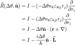
It is not as obvious how to determine the rotational operator compared to space and time translations. We may consider a special case (rotations about the x, y, or z-axis) then infer the general result, or use the general rotation matrix directly and tensor index notation with δij and εijk. To derive the infinitesimal rotation operator, which corresponds to small Δθ, we use the small angle approximations sin(Δθ) ≈ Δθ and cos(Δθ) ≈ 1, then Taylor expand about r or ri, keep the first order term, and substitute the angular momentum operator components.
, using the dot product  .
.
Again, a finite rotation can be made from lots of small rotations, replacing Δθ by Δθ/N and taking the limit as N tends to infinity gives the rotation operator for a finite rotation.
Rotations about the same axis do commute, for example a rotation through angles θ1 and θ2 about axis i can be written
In quantum mechanics, there is another form of rotation which mathematically appears similar to the orbital case, but has different properties, described next.
 . The eigenvalues of its components are the possible outcomes (in units of
  ) of a measurement of the spin projected onto one of the basis directions.
Rotations (of ordinary space) about an axis through angle θ about the unit vector  in space acting on a multicomponent wave function (spinor) at a point in space is represented by:
Evaluating the exponential for a given z-projection spin quantum number s gives a (2s + 1)-dimensional spin matrix. This can be used to define a spinor as a column vector of 2s + 1 components which transforms to a rotated coordinate system according to the spin matrix at a fixed point in space.
For the simplest non-trivial case of s = 1/2, the spin operator is given by
We have a similar rotation matrix:
Lorentz transformations can be parametrized by rapidity φ for a boost in the direction of a three-dimensional unit vector , and a rotation angle θ about a three-dimensional unit vector defining an axis, so
  and
and  are together six parameters of the Lorentz group (three for rotations and three for boosts). The Lorentz group is 6-dimensional.
 and generators J = (J1, J2, J3) for pure rotations are:
, are the boost transformation matrices. These matrices  and the corresponding generators K = (K1, K2, K3) are the remaining three group elements and generators of the Lorentz group:
The boost and rotation generators have representations denoted D(K) and D(J) respectively, the capital D in this context indicates a group representation.
For the Lorentz group, the representations D(K) and D(J) of the generators K and J fulfill the following commutation rules.
Under a proper orthochronous Lorentz transformation (r, t) → Λ(r, t) in Minkowski space, all one-particle quantum states ψσ locally transform under some representation D of the Lorentz group:[8] [9]
Applying this to particles with spin s;
In special relativity, space and time can be collected into a four-position vector X = (ct, −r), and in parallel so can energy and momentum which combine into a four-momentum vector P = (E/c, −p). With relativistic quantum mechanics in mind, the time duration and spatial displacement parameters (four in total, one for time and three for space) combine into a spacetime displacement ΔX = (cΔt, −Δr), and the energy and momentum operators are inserted in the four-momentum to obtain a four-momentum operator,
To describe spin in relativistic quantum mechanics, the Pauli–Lubanski pseudovector
 be a unitary operator, so the inverse is the Hermitian adjoint
  , which commutes with the Hamiltonian:
is conserved, and the Hamiltonian is invariant under the transformation .
Since the predictions of quantum mechanics should be invariant under the action of a group, physicists look for unitary transformations to represent the group.
Important subgroups of each U(N) are those unitary matrices which have unit determinant (or are "unimodular"): these are called the special unitary groups and are denoted SU(N).
The eight gluons states (8-dimensional column vectors) are simultaneous eigenstates of the adjoint representation of SU(3) , the 8-dimensional representation acting on its own Lie algebra su(3), for the λ3 and λ8 matrices. By forming tensor products of representations (the standard representation and its dual) and taking appropriate quotients, protons and neutrons, and other hadrons are eigenstates of various representations of SU(3) of color. The adjoint representation of above is isomorphic to the tensor product of the standard representation and its dual.
Charge conjugation switches particles and antiparticles. Physical laws and interactions unchanged by this operation have C symmetry.
The electromagnetic interaction is mediated by photons, which have no electric charge. The electromagnetic tensor has an electromagnetic four-potential field possessing gauge symmetry.
The strong (color) interaction is mediated by gluons, which can have eight color charges. There are eight gluon field strength tensors with corresponding gluon four potentials field, each possessing gauge symmetry.
 for a system of identical particles, the wave function
  must either remain the same or change sign upon such an exchange.
Because the exchange of two identical particles is mathematically equivalent to the rotation of each particle by 180 degrees (and so to the rotation of one particle's frame by 360 degrees),[12] the symmetric nature of the wave function depends on the particle's spin after the rotation operator is applied to it. Integer spin particles do not change the sign of their wave function upon a 360 degree rotation—therefore the sign of the wave function of the entire system does not change. Semi-integer spin particles change the sign of their wave function upon a 360 degree rotation (see more in spin–statistics theorem).
Particles for which the wave function does not change sign upon exchange are called bosons, or particles with a symmetric wave function. The particles for which the wave function of the system changes sign are called fermions, or particles with an antisymmetric wave function.
Fermions therefore obey different statistics (called Fermi–Dirac statistics) than bosons (which obey Bose–Einstein statistics). One of the consequences of Fermi–Dirac statistics is the exclusion principle for fermions—no two identical fermions can share the same quantum state (in other words, the wave function of two identical fermions in the same state is zero). This in turn results in degeneracy pressure for fermions—the strong resistance of fermions to compression into smaller volume. This resistance gives rise to the “stiffness” or “rigidity” of ordinary atomic matter (as atoms contain electrons which are fermions).
This article outlines the connection between the classical form of continuous symmetries as well as their quantum operators, and relates them to the Lie groups, and relativistic transformations in the Lorentz group, and Poincaré group.
Notation
The notational conventions used in this article are as follows. Boldface indicates vectors, four vectors, matrices, and vectorial operators, while quantum states use bra–ket notation. Wide hats are for operators, narrow hats are for unit vectors (including their components in tensor index notation). The summation convention on the repeated tensor indices is used, unless stated otherwise. The Minkowski metric signature is (+−−−).Symmetry transformations on the wavefunction in non-relativistic quantum mechanics
Continuous symmetries
Generally, the correspondence between continuous symmetries and conservation laws is given by Noether's theorem.The form of the fundamental quantum operators, for example energy as a partial time derivative and momentum as a spatial gradient, becomes clear when one considers the initial state, then changes one parameter of it slightly. This can be done for displacements (lengths), durations (time), and angles (rotations). Additionally, the invariance of certain quantities can be seen by making such changes in lengths and angles, which illustrates conservation of these quantities.
In what follows, transformations on only one-particle wavefunctions in the form:

 denotes a unitary operator. Unitarity is generally required for operators representing transformations of space, time, and spin, since the norm of a state (representing the total probability of finding the particle somewhere with some spin) must be invariant under these transformations. The inverse is the Hermitian conjugate
  . The results can be extended to many-particle wavefunctions. Written in Dirac notation as standard, the transformations on quantum state vectors are:
 changes ψ(r, t) to ψ(r′, t′), so the inverse
  changes ψ(r′, t′) back to ψ(r, t), so an operator
  invariant under satisfies:
![[\widehat{\Omega},\widehat{A}]\psi = 0](http://upload.wikimedia.org/math/7/a/a/7aa61324cf168fffc81a711667d977aa.png)
 .
.Overview of Lie group theory
Following are the key points of group theory relevant to quantum theory, examples are given throughout the article. For an alternative approach using matrix groups, see the books of Hall[1][2]Let G be a Lie group, which is a group parameterized by a finite number N of real continuously varying parameters ξ1, ξ2, ... ξN.
- the dimension of the group, N, is the number of parameters it has.
- the group elements, g, in G are functions of the parameters:
-
- and all parameters set to zero returns the identity element of the group:
- Group elements are often matrices which act on vectors, or transformations acting on functions.

- The generators of the group are the partial derivatives of the group elements with respect to the group parameters with the result evaluated when the parameter is set to zero:
-
- One aspect of generators in theoretical physics is they can be construed themselves as operators corresponding to symmetries, which may be written as matrices, or as differential operators. In quantum theory, for unitary representations of the group, the generators require a factor of i:
- The generators of the group form a vector space, which means linear combinations of generators also form a generator.


- The generators (whether matrices or differential operators) satisfy the commutator:
-
- where fabc are the (basis dependent) structure constants of the group. This makes, together with the vector space property, the set of all generators of a group a Lie algebra. Due to the antisymmetry of the bracket, the structure constants of the group are antisymmetric in the first two indices.
![\left[X_a,X_b\right] = i f_{abc}X_c](http://upload.wikimedia.org/math/5/3/7/537fd0dba4c904d03e541e87f9abb200.png)
- The representations of the group are denoted using a capital D and defined by:
-
- without summation on the repeated index j. Representations are linear operators that take in group elements and preserve the composition rule:
![D[g(\xi_j)] \equiv D(\xi_j) = e^{ i \xi_j D(X_j)}](http://upload.wikimedia.org/math/6/9/c/69ca103395123c0c89c05a32f9f65103.png)

- Representations also exist for the generators and the same notation of a capital D is used in this context: D(X). The D in the representation of a generator D(X) is not the same mapping as the D in a representation of a group element, nevertheless this notational abuse of using the same letter to denote two different mappings is used in the literature. An example of this abuse is to be found in the defining equation above.
Momentum and energy as generators of translation and time evolution, and rotation
The space translation operator acts on a wavefunction to shift the space coordinates by an infinitesimal displacement Δr. The explicit expression
  can be quickly determined by a Taylor expansion of ψ(r + Δr, t) about r, then (keeping the first order term and neglecting second and higher order terms), replace the space derivatives by the momentum operator
  . Similarly for the time translation operator acting on the time parameter, the Taylor expansion of ψ(r, t + Δt) is about t, and the time derivative replaced by the energy operator
  .
.Name Translation operator Time translation/evolution operator Action on wavefunction 

Infinitesimal operator 

Finite operator 

Generator Momentum operator 
Energy operator 


Space and time translations commute, which means the operators and generators commute.
Commutators Operators ![\left[\widehat{T}(\mathbf{r}_1), \widehat{T}(\mathbf{r}_2) \right] \psi(\mathbf{r},t) = 0](//upload.wikimedia.org/math/9/3/6/93673da4e82158114680695c93246592.png)
![\left[\widehat{U}(t_1), \widehat{U}(t_2) \right]\psi(\mathbf{r},t) = 0](//upload.wikimedia.org/math/0/b/0/0b05a056eb1aeaa52fcb81957a6b7057.png)
Generators ![\left[\widehat{p}_i,\widehat{p}_j,\right] \psi(\mathbf{r},t) = 0](//upload.wikimedia.org/math/9/f/f/9ffd09f9b4c23794f9a605732f41687c.png)
![\left[\widehat{E},\widehat{p}_i,\right] \psi(\mathbf{r},t) = 0](//upload.wikimedia.org/math/3/d/a/3da447d0ae1713ad6728d675306b928d.png)
![\left[\widehat{T}(\mathbf{r}_1), \widehat{T}(\mathbf{r}_2) \right] \psi(\mathbf{r},t) = 0](http://upload.wikimedia.org/math/9/3/6/93673da4e82158114680695c93246592.png)
![\left[\widehat{U}(t_1), \widehat{U}(t_2) \right]\psi(\mathbf{r},t) = 0](http://upload.wikimedia.org/math/0/b/0/0b05a056eb1aeaa52fcb81957a6b7057.png)
![\left[\widehat{p}_i,\widehat{p}_j,\right] \psi(\mathbf{r},t) = 0](http://upload.wikimedia.org/math/9/f/f/9ffd09f9b4c23794f9a605732f41687c.png)
![\left[\widehat{E},\widehat{p}_i,\right] \psi(\mathbf{r},t) = 0](http://upload.wikimedia.org/math/3/d/a/3da447d0ae1713ad6728d675306b928d.png)


An alternative notation is
 .
.Angular momentum as the generator of rotations
Orbital angular momentum
The rotation operator acts on a wavefunction to rotate the spatial coordinates of a particle by a constant angle Δθ:
 through an angular increment Δθ, given by:
 is a rotation matrix dependent on the axis and angle. In group theoretic language, the rotation matrices are group elements, and the angles and axis
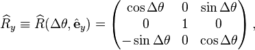
  are the parameters, of the three-dimensional special orthogonal group, SO(3). The rotation matrices about the standard Cartesian basis vector
  through angle Δθ, and the corresponding generators of rotations J = (Jx, Jy, Jz), are:


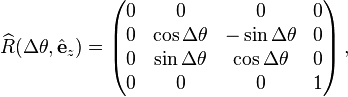
 , the rotation matrix elements are:[3]
![[\widehat{R}(\theta, \hat{\mathbf{n}})]_{ij} = (\delta_{ij} - n_i n_j) \cos\theta - \varepsilon_{ijk} n_k \sin\theta + n_i n_j](http://upload.wikimedia.org/math/2/d/9/2d9521c02693ce01780596dcb9d430d0.png)
It is not as obvious how to determine the rotational operator compared to space and time translations. We may consider a special case (rotations about the x, y, or z-axis) then infer the general result, or use the general rotation matrix directly and tensor index notation with δij and εijk. To derive the infinitesimal rotation operator, which corresponds to small Δθ, we use the small angle approximations sin(Δθ) ≈ Δθ and cos(Δθ) ≈ 1, then Taylor expand about r or ri, keep the first order term, and substitute the angular momentum operator components.
Rotation about 
Rotation about Action on wavefunction 

Infinitesimal operator 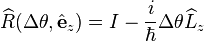
Infinitesimal rotations 
Same Finite rotations 
Same Generator z-component of the angular momentum operator 
Full angular momentum operator  .
.


 ., using the dot product
  .
.Again, a finite rotation can be made from lots of small rotations, replacing Δθ by Δθ/N and taking the limit as N tends to infinity gives the rotation operator for a finite rotation.
Rotations about the same axis do commute, for example a rotation through angles θ1 and θ2 about axis i can be written
![R(\theta_1 + \theta_2 , \mathbf{e}_i) = R(\theta_1 \mathbf{e}_i)R(\theta_2 \mathbf{e}_i)\,,\quad [R(\theta_1 \mathbf{e}_i),R(\theta_2 \mathbf{e}_i)]=0\,.](http://upload.wikimedia.org/math/e/3/8/e38e61c882333826ba27758639f55e29.png)
![[ L_i , L_j ] = i \hbar \varepsilon_{ijk} L_k.](http://upload.wikimedia.org/math/b/8/c/b8c35ce786859fe7a4220fc5498402b3.png)
In quantum mechanics, there is another form of rotation which mathematically appears similar to the orbital case, but has different properties, described next.
Spin angular momentum
All previous quantities have classical definitions. Spin is a quantity possessed by particles in quantum mechanics without any classical analogue, having the units of angular momentum. The spin vector operator is denoted . The eigenvalues of its components are the possible outcomes (in units of
  ) of a measurement of the spin projected onto one of the basis directions.
Rotations (of ordinary space) about an axis
through angle θ about the unit vector  in space acting on a multicomponent wave function (spinor) at a point in space is represented by:
Spin rotation operator (finite)


Evaluating the exponential for a given z-projection spin quantum number s gives a (2s + 1)-dimensional spin matrix. This can be used to define a spinor as a column vector of 2s + 1 components which transforms to a rotated coordinate system according to the spin matrix at a fixed point in space.
For the simplest non-trivial case of s = 1/2, the spin operator is given by


Total angular momentum
The total angular momentum operator is the sum of the orbital and spin
We have a similar rotation matrix:

Lorentz group in relativistic quantum mechanics
Following is an overview of the Lorentz group; a treatment of boosts and rotations in spacetime. Throughout this section, see (for example) T. Ohlsson (2011)[4] and E. Abers (2004).[5]Lorentz transformations can be parametrized by rapidity φ for a boost in the direction of a three-dimensional unit vector
 , and a rotation angle θ about a three-dimensional unit vector defining an axis, so
  and
and  are together six parameters of the Lorentz group (three for rotations and three for boosts). The Lorentz group is 6-dimensional.
Pure rotations in spacetime
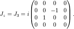
The rotation matrices and rotation generators considered above form the spacelike part of a four-dimensional matrix, representing pure-rotation Lorentz transformations. Three of the Lorentz group elements and generators J = (J1, J2, J3) for pure rotations are:


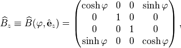
Pure boosts in spacetime
A boost with velocity ctanhφ in the x, y, or z directions given by the standard Cartesian basis vector, are the boost transformation matrices. These matrices  and the corresponding generators K = (K1, K2, K3) are the remaining three group elements and generators of the Lorentz group:


Combining boosts and rotations
Products of rotations give another rotation (a frequent exemplification of a subgroup), while products of boosts and boosts or of rotations and boosts cannot be expressed as pure boosts or pure rotations. In general, any Lorentz transformation can be expressed as a product of a pure rotation and a pure boost. For more background see (for example) B.R. Durney (2011)[6] and H.L. Berk et al.[7] and references therein.The boost and rotation generators have representations denoted D(K) and D(J) respectively, the capital D in this context indicates a group representation.
For the Lorentz group, the representations D(K) and D(J) of the generators K and J fulfill the following commutation rules.
Commutators Pure rotation Pure boost Lorentz transformation Generators ![\left[J_a ,J_b\right] = i\varepsilon_{abc}J_c](//upload.wikimedia.org/math/b/9/e/b9ef21752491d6efc5fd3c60159a3464.png)
![\left[K_a ,K_b\right] = -i\varepsilon_{abc}J_c](//upload.wikimedia.org/math/4/1/5/415431b2877f9f1d6d44cb931b79aab3.png)
![\left[J_a ,K_b\right] = i\varepsilon_{abc}K_c](//upload.wikimedia.org/math/c/c/9/cc9ecf8995440232a516d2e927be7471.png)
Representations ![\left[{D(J_a)} ,{D(J_b)}\right] = i\varepsilon_{abc}{D(J_c)}](//upload.wikimedia.org/math/e/f/e/efe92e77db683f518e55b022963e1e7e.png)
![\left[{D(K_a)} ,{D(K_b)}\right] = -i\varepsilon_{abc}{D(J_c)}](//upload.wikimedia.org/math/d/6/7/d6726cc086bdd8bdb439207cef2fae48.png)
![\left[{D(J_a)} ,{D(K_b)}\right] = i\varepsilon_{abc}{D(K_c)}](//upload.wikimedia.org/math/7/8/a/78a04b4ff381f160235763a9b7518c1e.png)
![\left[J_a ,J_b\right] = i\varepsilon_{abc}J_c](http://upload.wikimedia.org/math/b/9/e/b9ef21752491d6efc5fd3c60159a3464.png)
![\left[K_a ,K_b\right] = -i\varepsilon_{abc}J_c](http://upload.wikimedia.org/math/4/1/5/415431b2877f9f1d6d44cb931b79aab3.png)
![\left[J_a ,K_b\right] = i\varepsilon_{abc}K_c](http://upload.wikimedia.org/math/c/c/9/cc9ecf8995440232a516d2e927be7471.png)
![\left[{D(J_a)} ,{D(J_b)}\right] = i\varepsilon_{abc}{D(J_c)}](http://upload.wikimedia.org/math/e/f/e/efe92e77db683f518e55b022963e1e7e.png)
![\left[{D(K_a)} ,{D(K_b)}\right] = -i\varepsilon_{abc}{D(J_c)}](http://upload.wikimedia.org/math/d/6/7/d6726cc086bdd8bdb439207cef2fae48.png)
![\left[{D(J_a)} ,{D(K_b)}\right] = i\varepsilon_{abc}{D(K_c)}](http://upload.wikimedia.org/math/7/8/a/78a04b4ff381f160235763a9b7518c1e.png)
Transformation laws Pure boost Pure rotation Lorentz transformation Transformations 

![\Lambda(\varphi,\hat{\mathbf{a}},\theta,\hat{\mathbf{n}}) = \exp\left[-\frac{i}{\hbar} \left(\varphi\hat{\mathbf{a}} \cdot \mathbf{K} + \theta\hat{\mathbf{n}} \cdot \mathbf{J}\right)\right]](//upload.wikimedia.org/math/5/b/1/5b1105579de5e3dc8c453c61147821e9.png)
Representations ![D[\widehat{B}(\varphi,\hat{\mathbf{a}})] = \exp\left(-\frac{i}{\hbar} \varphi \hat{\mathbf{a}} \cdot D(\mathbf{K})\right)](//upload.wikimedia.org/math/d/0/5/d052ba9e0d997e0dfeb76a8756144f92.png)
![D[\widehat{R}(\theta,\hat{\mathbf{n}})] = \exp\left(-\frac{i}{\hbar}\theta \hat{\mathbf{n}} \cdot D(\mathbf{J})\right)](//upload.wikimedia.org/math/5/3/9/53994601ab414ef4e315925adf9440da.png)
![D[\Lambda(\theta,\hat{\mathbf{n}},\varphi,\hat{\mathbf{a}})] = \exp\left[-\frac{i}{\hbar}\left( \varphi \hat{\mathbf{a}} \cdot D(\mathbf{K}) + \theta \hat{\mathbf{n}} \cdot D(\mathbf{J})\right)\right]](//upload.wikimedia.org/math/c/8/4/c8482813c8b42b01de7e42110cc956c2.png)


![\Lambda(\varphi,\hat{\mathbf{a}},\theta,\hat{\mathbf{n}}) = \exp\left[-\frac{i}{\hbar} \left(\varphi\hat{\mathbf{a}} \cdot \mathbf{K} + \theta\hat{\mathbf{n}} \cdot \mathbf{J}\right)\right]](http://upload.wikimedia.org/math/5/b/1/5b1105579de5e3dc8c453c61147821e9.png)
![D[\widehat{B}(\varphi,\hat{\mathbf{a}})] = \exp\left(-\frac{i}{\hbar} \varphi \hat{\mathbf{a}} \cdot D(\mathbf{K})\right)](http://upload.wikimedia.org/math/d/0/5/d052ba9e0d997e0dfeb76a8756144f92.png)
![D[\widehat{R}(\theta,\hat{\mathbf{n}})] = \exp\left(-\frac{i}{\hbar}\theta \hat{\mathbf{n}} \cdot D(\mathbf{J})\right)](http://upload.wikimedia.org/math/5/3/9/53994601ab414ef4e315925adf9440da.png)
![D[\Lambda(\theta,\hat{\mathbf{n}},\varphi,\hat{\mathbf{a}})] = \exp\left[-\frac{i}{\hbar}\left( \varphi \hat{\mathbf{a}} \cdot D(\mathbf{K}) + \theta \hat{\mathbf{n}} \cdot D(\mathbf{J})\right)\right]](http://upload.wikimedia.org/math/c/8/4/c8482813c8b42b01de7e42110cc956c2.png)


![\Lambda(\varphi,\hat{\mathbf{a}}, \theta,\hat{\mathbf{n}}) = \exp\left(-\frac{i}{2}\omega_{\alpha\beta}M^{\alpha\beta}\right) = \exp \left[-\frac{i}{2}\left(\varphi \hat{\mathbf{a}} \cdot \mathbf{K} + \theta \hat{\mathbf{n}} \cdot \mathbf{J}\right)\right]](http://upload.wikimedia.org/math/3/b/1/3b17ce9822de3a7b1c427722259bb761.png)

Transformations of spinor wavefunctions in relativistic quantum mechanics
In relativistic quantum mechanics, wavefunctions are no longer single-component scalar fields, but now 2(2s + 1) component spinor fields, where s is the spin of the particle. The transformations of these functions in spacetime are given below.Under a proper orthochronous Lorentz transformation (r, t) → Λ(r, t) in Minkowski space, all one-particle quantum states ψσ locally transform under some representation D of the Lorentz group:[8] [9]


Real irreducible representations and spin
The irreducible representations of D(K) and D(J), in short "irreps", can be used to build to spin representations of the Lorentz group. Defining new operators:
![\left[A_i ,A_j\right] = \varepsilon_{ijk}A_k\,,\quad \left[B_i ,B_j\right] = \varepsilon_{ijk}B_k\,,\quad \left[A_i ,B_j\right] = 0\,,](http://upload.wikimedia.org/math/3/b/5/3b5b0fc86df99e55423bb0ddfe85f620.png)


Applying this to particles with spin s;
- left-handed (2s + 1)-component spinors transform under the real irreps D(s, 0),
- right-handed (2s + 1)-component spinors transform under the real irreps D(0, s),
- taking direct sums symbolized by ⊕ (see direct sum of matrices for the simpler matrix concept), one obtains the representations under which 2(2s + 1)-component spinors transform: D(m, n) ⊕ D(n, m) where m + n = s. These are also real irreps, but as shown above, they split into complex conjugates.
Relativistic wave equations
In the context of the Dirac equation and Weyl equation, the Weyl spinors satisfying the Weyl equation transform under the simplest irreducible spin representations of the Lorentz group, since the spin quantum number in this case is the smallest non-zero number allowed: 1/2. The 2-component left-handed Weyl spinor transforms under D(1/2, 0) and the 2-component right-handed Weyl spinor transforms under D(0, 1/2). Dirac spinors satisfying the Dirac equation transform under the representation D(1/2, 0) ⊕ D(0, 1/2), the direct sum of the irreps for the Weyl spinors.The Poincaré group in relativistic quantum mechanics and field theory
Space translations, time translations, rotations, and boosts, all taken together, constitute the Poincaré group. The group elements are the three rotation matrices and three boost matrices (as in the Lorentz group), and one for time translations and three for space translations in spacetime. There is a generator for each. Therefore the Poincaré group is 10-dimensional.In special relativity, space and time can be collected into a four-position vector X = (ct, −r), and in parallel so can energy and momentum which combine into a four-momentum vector P = (E/c, −p). With relativistic quantum mechanics in mind, the time duration and spatial displacement parameters (four in total, one for time and three for space) combine into a spacetime displacement ΔX = (cΔt, −Δr), and the energy and momentum operators are inserted in the four-momentum to obtain a four-momentum operator,

![\widehat{X}(\Delta \mathbf{X}) = \exp\left(-\frac{i}{\hbar}\Delta\mathbf{X}\cdot\widehat{\mathbf{P}}\right) = \exp\left[-\frac{i}{\hbar}\left(\Delta t\widehat{E} + \Delta \mathbf{r} \cdot\widehat{\mathbf{p}}\right)\right] \,.](http://upload.wikimedia.org/math/0/e/b/0eb62760e86a492105f79bd2f8a2c4c4.png)
![[P_\mu, P_\nu] = 0\,](http://upload.wikimedia.org/math/0/e/2/0e2d29720bdc47cab5c43ac422c3e02c.png)
![\frac{ 1 }{ i }[M_{\mu\nu}, P_\rho] = \eta_{\mu\rho} P_\nu - \eta_{\nu\rho} P_\mu\,](http://upload.wikimedia.org/math/f/4/0/f40121951f4049a34b814acd2555de99.png)
![\frac{ 1 }{ i }[M_{\mu\nu}, M_{\rho\sigma}] = \eta_{\mu\rho} M_{\nu\sigma} - \eta_{\mu\sigma} M_{\nu\rho} - \eta_{\nu\rho} M_{\mu\sigma} + \eta_{\nu\sigma} M_{\mu\rho}\,](http://upload.wikimedia.org/math/b/a/b/babb881fe999d7d65c429cd007087a27.png)
To describe spin in relativistic quantum mechanics, the Pauli–Lubanski pseudovector

![\left[P^{\mu},W^{\nu}\right]=0 \,,](http://upload.wikimedia.org/math/c/5/c/c5cc04203138fbf60da0fe6f92d4aec2.png)
![\left[J^{\mu \nu},W^{\rho}\right]=i \left( \eta^{\rho \nu} W^{\mu} - \eta^{\rho \mu} W^{\nu}\right) \,,](http://upload.wikimedia.org/math/0/b/d/0bd8d0a697644936a7d0938da89bb241.png)
![\left[W_{\mu},W_{\nu}\right]=-i \epsilon_{\mu \nu \rho \sigma} W^{\rho} P^{\sigma} \,.](http://upload.wikimedia.org/math/5/b/c/5bc6e51f25c9d32a042e05f4e949e419.png)
Symmetries in quantum field theory and particle physics
Unitary groups in quantum field theory
Group theory is an abstract way of mathematically analyzing symmetries. Unitary operators are paramount to quantum theory, so unitary groups are important in particle physics. The group of N dimensional unitary square matrices is denoted U(N). Unitary operators preserve inner products which means probabilities are also preserved, so the quantum mechanics of the system is invariant under unitary unitary transformations. Let be a unitary operator, so the inverse is the Hermitian adjoint
  , which commutes with the Hamiltonian:
![\left[\widehat{U}, \widehat{H} \right]=0](http://upload.wikimedia.org/math/5/e/d/5edb74f85bd0f00348482876839b3385.png) is conserved, and the Hamiltonian is invariant under the transformation .
is conserved, and the Hamiltonian is invariant under the transformation .Since the predictions of quantum mechanics should be invariant under the action of a group, physicists look for unitary transformations to represent the group.
Important subgroups of each U(N) are those unitary matrices which have unit determinant (or are "unimodular"): these are called the special unitary groups and are denoted SU(N).
U(1) and SU(1)
The simplest unitary group is U(1), which is just a complex number of modulus 1. This one-dimensional matrix entry is of the form:

U(2) and SU(2)
The general form of an element of a U(2) element is parametrized by two complex numbers a and b:

![[ \sigma_a , \sigma_b ] = 2i \hbar \varepsilon_{abc} \sigma_c](http://upload.wikimedia.org/math/c/a/2/ca28f375850ce697cf0a6d359204b5b7.png)

U(3) and SU(3)
The eight Gell-Mann matrices λn (see article for them and the structure constants) are important for quantum chromodynamics. They originally arose in the theory SU(3) of flavor which is still of practical importance in nuclear physics. They are the generators for the SU(3) group, so an element of SU(3) can be written analogously to an element of SU(2):
![\left[\lambda_a, \lambda_b \right] = 2i f_{abc}\lambda_c](http://upload.wikimedia.org/math/0/9/0/09040bcbb9cb0391005466a03da2a680.png)

The eight gluons states (8-dimensional column vectors) are simultaneous eigenstates of the adjoint representation of SU(3) , the 8-dimensional representation acting on its own Lie algebra su(3), for the λ3 and λ8 matrices. By forming tensor products of representations (the standard representation and its dual) and taking appropriate quotients, protons and neutrons, and other hadrons are eigenstates of various representations of SU(3) of color. The adjoint representation of above is isomorphic to the tensor product of the standard representation and its dual.
Matter and antimatter
In relativistic quantum mechanics, relativistic wave equations predict a remarkable symmetry of nature: that every particle has a corresponding antiparticle. This is mathematically contained in the spinor fields which are the solutions of the relativistic wave equations.Charge conjugation switches particles and antiparticles. Physical laws and interactions unchanged by this operation have C symmetry.
Discrete spacetime symmetries
- Parity mirrors the orientation of the spatial coordinates from left-handed to right-handed. Informally, space is "reflected" into its mirror image. Physical laws and interactions unchanged by this operation have P symmetry.
- Time reversal negates the time coordinate, which amounts to time running from future to past. A curious property of time, which space does not have, is that it is unidirectional: particles traveling forwards in time are equivalent to antiparticles traveling back in time. Physical laws and interactions unchanged by this operation have T symmetry.
C, P, T symmetries
Gauge theory
In quantum electrodynamics, the symmetry group is U(1) and is abelian. In quantum chromodynamics, the symmetry group is SU(3) and is non-abelian.The electromagnetic interaction is mediated by photons, which have no electric charge. The electromagnetic tensor has an electromagnetic four-potential field possessing gauge symmetry.
The strong (color) interaction is mediated by gluons, which can have eight color charges. There are eight gluon field strength tensors with corresponding gluon four potentials field, each possessing gauge symmetry.
The strong (color) interaction
Color charge
Analogous to the spin operator, there are color charge operators in terms of the Gell-Mann matrices λj:
![\left[\hat{F}_j,\hat{H}\right] = 0](http://upload.wikimedia.org/math/1/d/4/1d4aa114005d71fcacb98f8a3d3d39c4.png)
Isospin
Isospin is conserved in strong interactions.The weak and electromagnetic interactions
Duality transformation
Magnetic monopoles can be theoretically realized, although current observations and theory are consistent with them existing or not existing. Electric and magnetic charges can effectively be "rotated into one another" by a duality transformation.Electroweak symmetry
Supersymmetry
A Lie superalgebra is an algebra in which (suitable) basis elements either have a commutation relation or have an anticommutation relation. Symmetries have been proposed to the effect that all fermionic particles have bosonic analogues, and vice versa. These symmetry have theoretical appeal in that no extra assumptions (such as existence of strings) barring symmetries are made. In addition, by assuming supersymmetry, a number puzzling issues can be resolved. These symmetries, which are represented by Lie superalgebras, have not been confirmed experimentally. It is now believed that they are broken symmetries, if they exist. But it has been speculated that dark matter is constitutes gravitinos, a spin 3/2 particle with mass, its supersymmetric partner being the graviton.Exchange symmetry
The concept of exchange symmetry is derived from a fundamental postulate of quantum statistics, which states that no observable physical quantity should change after exchanging two identical particles. It states that because all observables are proportional to for a system of identical particles, the wave function
  must either remain the same or change sign upon such an exchange.
Because the exchange of two identical particles is mathematically equivalent to the rotation of each particle by 180 degrees (and so to the rotation of one particle's frame by 360 degrees),[12] the symmetric nature of the wave function depends on the particle's spin after the rotation operator is applied to it. Integer spin particles do not change the sign of their wave function upon a 360 degree rotation—therefore the sign of the wave function of the entire system does not change. Semi-integer spin particles change the sign of their wave function upon a 360 degree rotation (see more in spin–statistics theorem).
Particles for which the wave function does not change sign upon exchange are called bosons, or particles with a symmetric wave function. The particles for which the wave function of the system changes sign are called fermions, or particles with an antisymmetric wave function.
Fermions therefore obey different statistics (called Fermi–Dirac statistics) than bosons (which obey Bose–Einstein statistics). One of the consequences of Fermi–Dirac statistics is the exclusion principle for fermions—no two identical fermions can share the same quantum state (in other words, the wave function of two identical fermions in the same state is zero). This in turn results in degeneracy pressure for fermions—the strong resistance of fermions to compression into smaller volume. This resistance gives rise to the “stiffness” or “rigidity” of ordinary atomic matter (as atoms contain electrons which are fermions).

 is the quark field, a dynamical function of spacetime, in the
  ;
;  are the
  represents the gauge invariant

 , which represents some kind of "stiffness" of the interaction between the particle and its anti-particle at large distances, similar to the
  is proportional to the area enclosed by the loop. For this behaviour the non-abelian behaviour of the gauge group is essential.
 for i =1,...,N, with the special fixed "random" couplings
  Here the εi and εk quantities can independently and "randomly" take the values ±1, which corresponds to a most-simple gauge transformation
  This means that thermodynamic expectation values of measurable quantities, e.g. of the energy
  are invariant.
 , which in the QCD correspond to the gluons, are "frozen" to fixed values (quenching). In contrast, in the QCD they "fluctuate" (annealing), and through the large number of gauge degrees of freedom the
  along a closed loop W. However, for a Mattis spin glass – in contrast to "genuine" spin glasses – the quantity PW never becomes negative.
 (where Rc is a characteristic correlation length for the glued loops, corresponding to the above-mentioned "bag radius", while λw is the wavelength of an excitation) any non-trivial correlation vanishes totally, as if the system had crystallized.
 on the r.h.s. of the Lagrangian.


