From Wikipedia, the free encyclopedia


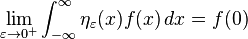
The Dirac delta function as the limit (in the sense of distributions) of the sequence of zero-centered normal distributions 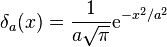 as
as  .
.
 as
as  .
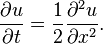
.In mathematics, the Dirac delta function, or δ function, is a generalized function, or distribution, on the real number line that is zero everywhere except at zero, with an integral of one over the entire real line.[1][2][3] The delta function is sometimes thought of as an infinitely high, infinitely thin spike at the origin, with total area one under the spike, and physically represents the density of an idealized point mass or point charge.[4] It was introduced by theoretical physicist Paul Dirac. In the context of signal processing it is often referred to as the unit impulse symbol (or function).[5] Its discrete analog is the Kronecker delta function, which is usually defined on a discrete domain and takes values 0 and 1.
From a purely mathematical viewpoint, the Dirac delta is not strictly a function, because any extended-real function that is equal to zero everywhere but a single point must have total integral zero.[6] The delta function only makes sense as a mathematical object when it appears inside an integral. While from this perspective the Dirac delta can usually be manipulated as though it were a function, formally it must be defined as a distribution that is also a measure. In many applications, the Dirac delta is regarded as a kind of limit (a weak limit) of a sequence of functions having a tall spike at the origin. The approximating functions of the sequence are thus "approximate" or "nascent" delta functions.
Overview
The graph of the delta function is usually thought of as following the whole x-axis and the positive y-axis. Despite its name, the delta function is not truly a function, at least not a usual one with range in real numbers. For example, the objects f(x) = δ(x) and g(x) = 0 are equal everywhere except at x = 0 yet have integrals that are different.According to Lebesgue integration theory, if f and g are functions such that f = g almost everywhere, then f is integrable if and only if g is integrable and the integrals of f and g are identical. Rigorous treatment of the Dirac delta requires measure theory or the theory of distributions.
The Dirac delta is used to model a tall narrow spike function (an impulse), and other similar abstractions such as a point charge, point mass or electron point. For example, to calculate the dynamics of a baseball being hit by a bat, one can approximate the force of the bat hitting the baseball by a delta function. In doing so, one not only simplifies the equations, but one also is able to calculate the motion of the baseball by only considering the total impulse of the bat against the ball rather than requiring knowledge of the details of how the bat transferred energy to the ball.
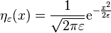
In applied mathematics, the delta function is often manipulated as a kind of limit (a weak limit) of a sequence of functions, each member of which has a tall spike at the origin: for example, a sequence of Gaussian distributions centered at the origin with variance tending to zero.
History
Joseph Fourier presented what is now called the Fourier integral theorem in his treatise Théorie analytique de la chaleur in the form:[7]


As justified using the theory of distributions, the Cauchy equation can be rearranged to resemble Fourier's original formulation and expose the δ-function as:


- The greatest drawback of the classical Fourier transformation is a rather narrow class of functions (originals) for which it can be effectively computed. Namely, it is necessary that these functions decrease sufficiently rapidly to zero (in the neighborhood of infinity) in order to insure the existence of the Fourier integral. For example, the Fourier transform of such simple functions as polynomials does not exist in the classical sense. The extension of the classical Fourier transformation to distributions considerably enlarged the class of functions that could be transformed and this removed many obstacles.
An infinitesimal formula for an infinitely tall, unit impulse delta function (infinitesimal version of Cauchy distribution) explicitly appears in an 1827 text of Augustin Louis Cauchy.[15] Siméon Denis Poisson considered the issue in connection with the study of wave propagation as did Gustav Kirchhoff somewhat later. Kirchhoff and Hermann von Helmholtz also introduced the unit impulse as a limit of Gaussians, which also corresponded to Lord Kelvin's notion of a point heat source. At the end of the 19th century, Oliver Heaviside used formal Fourier series to manipulate the unit impulse.[16] The Dirac delta function as such was introduced as a "convenient notation" by Paul Dirac in his influential 1930 book The Principles of Quantum Mechanics.[17] He called it the "delta function" since he used it as a continuous analogue of the discrete Kronecker delta.
Definitions
The Dirac delta can be loosely thought of as a function on the real line which is zero everywhere except at the origin, where it is infinite,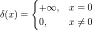
This is merely a heuristic characterization. The Dirac delta is not a function in the traditional sense as no function defined on the real numbers has these properties.[17] The Dirac delta function can be rigorously defined either as a distribution or as a measure.

As a measure
One way to rigorously define the delta function is as a measure, which accepts as an argument a subset A of the real line R, and returns δ(A) = 1 if 0 ∈ A, and δ(A) = 0 otherwise.[19] If the delta function is conceptualized as modeling an idealized point mass at 0, then δ(A) represents the mass contained in the set A. One may then define the integral against δ as the integral of a function against this mass distribution. Formally, the Lebesgue integral provides the necessary analytic device. The Lebesgue integral with respect to the measure δ satisfies

As a probability measure on R, the delta measure is characterized by its cumulative distribution function, which is the unit step function[21]

![H(x) = \int_{\mathbf{R}}\mathbf{1}_{(-\infty,x]}(t)\,\delta\{dt\} = \delta(-\infty,x].](http://upload.wikimedia.org/math/9/8/7/987eedd63c58e74c47a2c8f50958a5bf.png)

As a distribution
In the theory of distributions a generalized function is thought of not as a function itself, but only in relation to how it affects other functions when it is "integrated" against them. In keeping with this philosophy, to define the delta function properly, it is enough to say what the "integral" of the delta function against a sufficiently "good" test function is. If the delta function is already understood as a measure, then the Lebesgue integral of a test function against that measure supplies the necessary integral.A typical space of test functions consists of all smooth functions on R with compact support. As a distribution, the Dirac delta is a linear functional on the space of test functions and is defined by[23]
![\delta[\varphi] = \varphi(0)\,](//upload.wikimedia.org/math/b/1/c/b1c2074d920e293f6ee23fc02130a233.png) (1)
(1)
![\delta[\varphi] = \varphi(0)\,](http://upload.wikimedia.org/math/b/1/c/b1c2074d920e293f6ee23fc02130a233.png)
For δ to be properly a distribution, it must be "continuous" in a suitable sense. In general, for a linear functional S on the space of test functions to define a distribution, it is necessary and sufficient that, for every positive integer N there is an integer MN and a constant CN such that for every test function φ, one has the inequality[24]
![|S[\phi]| \le C_N \sum_{k=0}^{M_N}\sup_{x\in [-N,N]}|\phi^{(k)}(x)|.](http://upload.wikimedia.org/math/0/3/0/030ace79cd564b4f45e9d7083e118018.png)
The delta distribution can also be defined in a number of equivalent ways. For instance, it is the distributional derivative of the Heaviside step function. This means that, for every test function φ, one has
![\delta[\phi] = -\int_{-\infty}^\infty \phi'(x)H(x)\, dx.](http://upload.wikimedia.org/math/4/9/c/49c836b66863ded1069bba1f2c224c2c.png)


Generalizations
The delta function can be defined in n-dimensional Euclidean space Rn as the measure such that
 (2)
(2)

However, despite widespread use in engineering contexts, (2) should be manipulated with care, since the product of distributions can only be defined under quite narrow circumstances.[26]
The notion of a Dirac measure makes sense on any set.[19] Thus if X is a set, x0 ∈ X is a marked point, and Σ is any sigma algebra of subsets of X, then the measure defined on sets A ∈ Σ by

Another common generalization of the delta function is to a differentiable manifold where most of its properties as a distribution can also be exploited because of the differentiable structure. The delta function on a manifold M centered at the point x0 ∈ M is defined as the following distribution:
![\delta_{x_0}[\phi] = \phi(x_0)](//upload.wikimedia.org/math/1/e/b/1eb3281ef2f90360471468f213e873b4.png) (3)
(3)
![\delta_{x_0}[\phi] = \phi(x_0)](http://upload.wikimedia.org/math/1/e/b/1eb3281ef2f90360471468f213e873b4.png)
On a locally compact Hausdorff space X, the Dirac delta measure concentrated at a point x is the Radon measure associated with the Daniell integral (3) on compactly supported continuous functions φ. At this level of generality, calculus as such is no longer possible, however a variety of techniques from abstract analysis are available. For instance, the mapping
 is a continuous embedding of X into the space of finite Radon measures on X, equipped with its vague topology. Moreover, the convex hull of the image of X under this embedding is dense in the space of probability measures on X.[28]
Properties
Scaling and symmetry
The delta function satisfies the following scaling property for a non-zero scalar α:[29]
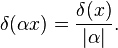 (4)
(4)

Algebraic properties
The distributional product of δ with x is equal to zero:
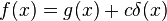
Translation
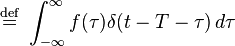
The integral of the time-delayed Dirac delta is given by:
It follows that the effect of convolving a function f(t) with the time-delayed Dirac delta is to time-delay f(t) by the same amount:

 (using (4):
 )
)


This holds under the precise condition that f be a tempered distribution (see the discussion of the Fourier transform below). As a special case, for instance, we have the identity (understood in the distribution sense)
Composition with a function
More generally, the delta distribution may be composed with a smooth function g(x) in such a way that the familiar change of variables formula holds, that
 so that this identity holds for all compactly supported test functions f. Therefore, the domain must be broken up to exclude the g' = 0 point. This distribution satisfies δ(g(x)) = 0 if g′ is nowhere zero, and otherwise if g has a real root at x0, then

![\delta\left(x^2-\alpha^2\right) = \frac{1}{2|\alpha|}\Big[\delta\left(x+\alpha\right)+\delta\left(x-\alpha\right)\Big].](http://upload.wikimedia.org/math/7/6/b/76bffc74318764a82234cf20e87ef2d2.png)

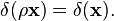
Properties in n dimensions
The delta distribution in an n-dimensional space satisfies the following scaling property instead:

Using the coarea formula from geometric measure theory, one can also define the composition of the delta function with a submersion from one Euclidean space to another one of different dimension; the result is a type of current. In the special case of a continuously differentiable function g: Rn → R such that the gradient of g is nowhere zero, the following identity holds[34]
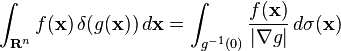
More generally, if S is a smooth hypersurface of Rn, then we can associated to S the distribution that integrates any compactly supported smooth function g over S:
![\delta_S[g] = \int_S g(\mathbf{s})\,d\sigma(\mathbf{s})](http://upload.wikimedia.org/math/6/c/9/6c9c04f375fe130586088421d27e4a54.png)

Fourier transform
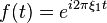
The delta function is a tempered distribution, and therefore it has a well-defined Fourier transform. Formally, one finds[37]

 of tempered distributions with Schwartz functions. Thus
  is defined as the unique tempered distribution satisfying

As a result of this identity, the convolution of the delta function with any other tempered distribution S is simply S:

The inverse Fourier transform of the tempered distribution f(ξ) = 1 is the delta function. Formally, this is expressed


In these terms, the delta function provides a suggestive statement of the orthogonality property of the Fourier kernel on R. Formally, one has
![\int_{-\infty}^\infty e^{i 2\pi \xi_1 t} \left[e^{i 2\pi \xi_2 t}\right]^*\,dt = \int_{-\infty}^\infty e^{-i 2\pi (\xi_2 - \xi_1) t} \,dt = \delta(\xi_2 - \xi_1).](http://upload.wikimedia.org/math/9/0/c/90c2db7fc675792938b3e30c140a002c.png)

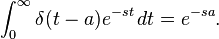
By analytic continuation of the Fourier transform, the Laplace transform of the delta function is found to be[38]
Distributional derivatives
The distributional derivative of the Dirac delta distribution is the distribution δ′ defined on compactly supported smooth test functions φ by[39]![\delta'[\varphi] = -\delta[\varphi']=-\varphi'(0).](http://upload.wikimedia.org/math/4/7/1/471945b0e4a22d140cb57d2852cb7469.png)

![\delta^{(k)}[\varphi] = (-1)^k \varphi^{(k)}(0).](http://upload.wikimedia.org/math/3/4/0/340c88866e5e9644a083eb073f44da09.png)
The first derivative of the delta function is the distributional limit of the difference quotients:[40]

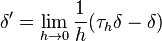
![(\tau_h S)[\varphi] = S[\tau_{-h}\varphi].](http://upload.wikimedia.org/math/5/8/2/582370f779f7278f90c4edd8dd1b2632.png)
The derivative of the delta function satisfies a number of basic properties, including:
Furthermore, the convolution of δ′ with a compactly supported smooth function f is


Higher dimensions
More generally, on an open set U in the n-dimensional Euclidean space Rn, the Dirac delta distribution centered at a point a ∈ U is defined by[43]![\delta_a[\phi]=\phi(a)](http://upload.wikimedia.org/math/0/6/f/06f5bf5d607c7c7cd5b4a20cb5a935be.png)

The first partial derivatives of the delta function are thought of as double layers along the coordinate planes. More generally, the normal derivative of a simple layer supported on a surface is a double layer supported on that surface, and represents a laminar magnetic monopole. Higher derivatives of the delta function are known in physics as multipoles.
Higher derivatives enter into mathematics naturally as the building blocks for the complete structure of distributions with point support. If S is any distribution on U supported on the set {a} consisting of a single point, then there is an integer m and coefficients cα such that[44]

Representations of the delta function
The delta function can be viewed as the limit of a sequence of functions
 (5)
(5)

Approximations to the identity
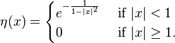
Typically a nascent delta function ηε can be constructed in the following manner. Let η be an absolutely integrable function on R of total integral 1, and define

The ηε constructed in this way are known as an approximation to the identity.[46] This terminology is because the space L1(R) of absolutely integrable functions is closed under the operation of convolution of functions: f ∗ g ∈ L1(R) whenever f and g are in L1(R). However, there is no identity in L1(R) for the convolution product: no element h such that f ∗ h = f for all f. Nevertheless, the sequence ηε does approximate such an identity in the sense that

If the initial η = η1 is itself smooth and compactly supported then the sequence is called a mollifier. The standard mollifier is obtained by choosing η to be a suitably normalized bump function, for instance
Probabilistic considerations
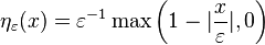
In the context of probability theory, it is natural to impose the additional condition that the initial η1 in an approximation to the identity should be positive, as such a function then represents a probability distribution. Convolution with a probability distribution is sometimes favorable because it does not result in overshoot or undershoot, as the output is a convex combination of the input values, and thus falls between the maximum and minimum of the input function. Taking η1 to be any probability distribution at all, and letting ηε(x) = η1(x/ε)/ε as above will give rise to an approximation to the identity. In general this converges more rapidly to a delta function if, in addition, η has mean 0 and has small higher moments. For instance, if η1 is the uniform distribution on [−1/2, 1/2], also known as the rectangular function, then:[48]

Semigroups
Nascent delta functions often arise as convolution semigroups. This amounts to the further constraint that the convolution of ηε with ηδ must satisfy
In practice, semigroups approximating the delta function arise as fundamental solutions or Green's functions to physically motivated elliptic or parabolic partial differential equations. In the context of applied mathematics, semigroups arise as the output of a linear time-invariant system. Abstractly, if A is a linear operator acting on functions of x, then a convolution semigroup arises by solving the initial value problem

Some examples of physically important convolution semigroups arising from such a fundamental solution include the following.
- The heat kernel
In higher-dimensional Euclidean space Rn, the heat kernel is

The Poisson kernel


 = |2\pi\xi|\mathcal{F}f(\xi).](http://upload.wikimedia.org/math/0/e/f/0efbf9975afcefde8ede21bb02688b9d.png)
Oscillatory integrals
In areas of physics such as wave propagation and wave mechanics, the equations involved are hyperbolic and so may have more singular solutions. As a result, the nascent delta functions that arise as fundamental solutions of the associated Cauchy problems are generally oscillatory integrals. An example, which comes from a solution of the Euler–Tricomi equation of transonic gas dynamics,[50] is the rescaled Airy function
Another example is the Cauchy problem for the wave equation in R1+1:[51]

Other approximations to the identity of this kind include the sinc function (used widely in electronics and telecommunications)


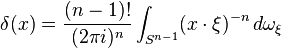
Plane wave decomposition
One approach to the study of a linear partial differential equation![L[u]=f,\,](http://upload.wikimedia.org/math/1/8/9/1892330c3bf4359ba7d85f5477cd1dc5.png)
![L[u]=\delta.\,](http://upload.wikimedia.org/math/5/b/9/5b90740ee993fff2fc4ab43ea58ea0f5.png)
![L[u]=h\,](http://upload.wikimedia.org/math/d/5/4/d5479eae1f42c7bce59de2431206a266.png)

Such a decomposition of the delta function into plane waves was part of a general technique first introduced essentially by Johann Radon, and then developed in this form by Fritz John (1955).[52] Choose k so that n + k is an even integer, and for a real number s, put
![g(s) = \operatorname{Re}\left[\frac{-s^k\log(-is)}{k!(2\pi i)^n}\right]
=\begin{cases}
\frac{|s|^k}{4k!(2\pi i)^{n-1}}&n \text{ odd}\\
&\\
-\frac{|s|^k\log|s|}{k!(2\pi i)^{n}}&n \text{ even.}
\end{cases}](http://upload.wikimedia.org/math/d/a/f/daf762b8ac926ae73edf7d238bab1787.png)


Fourier kernels
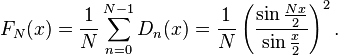
In the study of Fourier series, a major question consists of determining whether and in what sense the Fourier series associated with a periodic function converges to the function. The nth partial sum of the Fourier series of a function f of period 2π is defined by convolution (on the interval [−π,π]) with the Dirichlet kernel: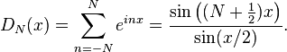


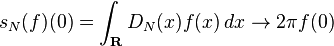

In spite of this, the result does not hold for all compactly supported continuous functions: that is DN does not converge weakly in the sense of measures. The lack of convergence of the Fourier series has led to the introduction of a variety of summability methods in order to produce convergence. The method of Cesàro summation leads to the Fejér kernel[53]

Hilbert space theory
The Dirac delta distribution is a densely defined unbounded linear functional on the Hilbert space L2 of square integrable functions. Indeed, smooth compactly support functions are dense in L2, and the action of the delta distribution on such functions is well-defined. In many applications, it is possible to identify subspaces of L2 and to give a stronger topology on which the delta function defines a bounded linear functional.- Sobolev spaces

![\delta[f]=|f(0)| < C \|f\|_{H^1}.](http://upload.wikimedia.org/math/d/0/4/d041f4205de07df754884b550badb5ba.png)
Spaces of holomorphic functions
In complex analysis, the delta function enters via Cauchy's integral formula which asserts that if D is a domain in the complex plane with smooth boundary, then
![\delta_z[f] = f(z) = \frac{1}{2\pi i} \oint_{\partial D} \frac{f(\zeta)\,d\zeta}{\zeta-z}.](http://upload.wikimedia.org/math/b/7/9/b791831a2283ea47b3ee2a7a27ecea0e.png)
Resolutions of the identity
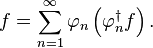
Given a complete orthonormal basis set of functions {φn} in a separable Hilbert space, for example, the normalized eigenvectors of a compact self-adjoint operator, any vector f can be expressed as:


Infinitesimal delta functions
Cauchy used an infinitesimal α to write down a unit impulse, infinitely tall and narrow Dirac-type delta function δα satisfying in a number of articles in 1827.[59] Cauchy defined an infinitesimal in Cours d'Analyse (1827) in terms of a sequence tending to zero. Namely, such a null sequence becomes an infinitesimal in Cauchy's and Lazare Carnot's terminology.
Non-standard analysis allows one to rigorously treat infinitesimals. The article by Yamashita (2007) contains a bibliography on modern Dirac delta functions in the context of an infinitesimal-enriched continuum provided by the hyperreals. Here the Dirac delta can be given by an actual function, having the property that for every real function F one has
as anticipated by Fourier and Cauchy.Dirac comb

A so-called uniform "pulse train" of Dirac delta measures, which is known as a Dirac comb, or as the Shah distribution, creates a sampling function, often used in digital signal processing (DSP) and discrete time signal analysis. The Dirac comb is given as the infinite sum, whose limit is understood in the distribution sense,

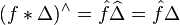
Up to an overall normalizing constant, the Dirac comb is equal to its own Fourier transform. This is significant because if f is any Schwartz function, then the periodization of f is given by the convolution

Sokhotski–Plemelj theorem
The Sokhotski–Plemelj theorem, important in quantum mechanics, relates the delta function to the distribution p.v.1/x, the Cauchy principal value of the function 1/x, defined by


Relationship to the Kronecker delta
The Kronecker delta δij is the quantity defined by
 is any doubly infinite sequence, then

Applications
Probability theory
In probability theory and statistics, the Dirac delta function is often used to represent a discrete distribution, or a partially discrete, partially continuous distribution, using a probability density function (which is normally used to represent fully continuous distributions). For example, the probability density function f(x) of a discrete distribution consisting of points x = {x1, ..., xn}, with corresponding probabilities p1, ..., pn, can be written as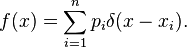


![\ell(x,t) = \lim_{\varepsilon\to 0^+}\frac{1}{2\varepsilon}\int_0^t \mathbf{1}_{[x-\varepsilon,x+\varepsilon]}(B(s))\,ds](http://upload.wikimedia.org/math/7/c/7/7c752721694494c477e28c4a377f2e38.png)
Quantum mechanics
We give an example of how the delta function is expedient in quantum mechanics. The wave function of a particle gives the probability amplitude of finding a particle within a given region of space. Wave functions are assumed to be elements of the Hilbert space L2 of square-integrable functions, and the total probability of finding a particle within a given interval is the integral of the magnitude of the wave function squared over the interval. A set {φn} of wave functions is orthonormal if they are normalized by

 . Complete orthonormal systems of wave functions appear naturally as the eigenfunctions of the Hamiltonian (of a bound system) in quantum mechanics that measures the energy levels, which are called the eigenvalues. The set of eigenvalues, in this case, is known as the spectrum of the Hamiltonian. In bra–ket notation, as above, this equality implies the resolution of the identity:

 in Dirac notation, and are known as position eigenstates.
Similar considerations apply to the eigenstates of the momentum operator, or indeed any other self-adjoint unbounded operator P on the Hilbert space, provided the spectrum of P is continuous and there are no degenerate eigenvalues. In that case, there is a set Ω of real numbers (the spectrum), and a collection φy of distributions indexed by the elements of Ω, such that


The delta function also has many more specialized applications in quantum mechanics, such as the delta potential models for a single and double potential well.
Structural mechanics
The delta function can be used in structural mechanics to describe transient loads or point loads acting on structures. The governing equation of a simple mass–spring system excited by a sudden force impulse I at time t = 0 can be written
As another example, the equation governing the static deflection of a slender beam is, according to Euler–Bernoulli theory,


Also a point moment acting on a beam can be described by delta functions. Consider two opposing point forces F at a distance d apart. They then produce a moment M = Fd acting on the beam. Now, let the distance d approach the limit zero, while M is kept constant. The load distribution, assuming a clockwise moment acting at x = 0, is written


