Search This Blog

Thursday, May 14, 2015

Noether's theorem


From Wikipedia, the free encyclopedia


Emmy Noether was an influential German mathematician known for her groundbreaking contributions to abstract algebra and theoretical physics.

Noether's (first) theorem states that every differentiable symmetry of the action of a physical system has a corresponding conservation law. The theorem was proven by German mathematician Emmy Noether in 1915 and published in 1918.[1] The action of a physical system is the integral over time of a Lagrangian function (which may or may not be an integral over space of a Lagrangian density function), from which the system's behavior can be determined by the principle of least action.

Noether's theorem has become a fundamental tool of modern theoretical physics and the calculus of variations. A generalization of the seminal formulations on constants of motion in Lagrangian and Hamiltonian mechanics (developed in 1788 and 1833, respectively), it does not apply to systems that cannot be modeled with a Lagrangian alone (e.g. systems with a Rayleigh dissipation function). In particular, dissipative systems with continuous symmetries need not have a corresponding conservation law.

Basic illustrations and background

As an illustration, if a physical system behaves the same regardless of how it is oriented in space, its Lagrangian is rotationally symmetric: from this symmetry, Noether's theorem dictates that the angular momentum of the system be conserved, as a consequence of its laws of motion. The physical system itself need not be symmetric; a jagged asteroid tumbling in space conserves angular momentum despite its asymmetry — it is the laws of its motion that are symmetric.

As another example, if a physical process exhibits the same outcomes regardless of place or time, then its Lagrangian is symmetric under continuous translations in space and time: by Noether's theorem, these symmetries account for the conservation laws of linear momentum and energy within this system, respectively.


Noether's theorem is important, both because of the insight it gives into conservation laws, and also as a practical calculational tool. It allows investigators to determine the conserved quantities (invariants) from the observed symmetries of a physical system. Conversely, it allows researchers to consider whole classes of hypothetical Lagrangians with given invariants, to describe a physical system. As an illustration, suppose that a new field is discovered that conserves a quantity X. Using Noether's theorem, the types of Lagrangians that conserve X through a continuous symmetry may be determined, and their fitness judged by further criteria.

There are numerous versions of Noether's theorem, with varying degrees of generality. The original version only applied to ordinary differential equations (particles) and not partial differential equations (fields). The original versions also assume that the Lagrangian only depends upon the first derivative, while later versions generalize the theorem to Lagrangians depending on the nth derivative.[disputed ] There are natural quantum counterparts of this theorem, expressed in the Ward–Takahashi identities. Generalizations of Noether's theorem to superspaces are also available.

Informal statement of the theorem

All fine technical points aside, Noether's theorem can be stated informally
If a system has a continuous symmetry property, then there are corresponding quantities whose values are conserved in time.[2]
A more sophisticated version of the theorem involving fields states that:
To every differentiable symmetry generated by local actions, there corresponds a conserved current.
The word "symmetry" in the above statement refers more precisely to the covariance of the form that a physical law takes with respect to a one-dimensional Lie group of transformations satisfying certain technical criteria. The conservation law of a physical quantity is usually expressed as a continuity equation.

The formal proof of the theorem utilizes the condition of invariance to derive an expression for a current associated with a conserved physical quantity. In modern (since ca. 1980[3]) terminology, the conserved quantity is called the Noether charge, while the flow carrying that charge is called the Noether current. The Noether current is defined up to a solenoidal (divergenceless) vector field.

In the context of gravitation, Felix Klein's statement of Noether's theorem for action I stipulates for the invariants:[4]
If an integral I is invariant under a continuous group Gρ with ρ parameters, then ρ linearly independent combinations of the Lagrangian expressions are divergences.

Historical context

A conservation law states that some quantity X in the mathematical description of a system's evolution remains constant throughout its motion — it is an invariant. Mathematically, the rate of change of X (its derivative with respect to time) vanishes,
\frac{dX}{dt} = 0 ~.
Such quantities are said to be conserved; they are often called constants of motion (although motion per se need not be involved, just evolution in time). For example, if the energy of a system is conserved, its energy is invariant at all times, which imposes a constraint on the system's motion and may help solving for it. Aside from insights that such constants of motion give into the nature of a system, they are a useful calculational tool; for example, an approximate solution can be corrected by finding the nearest state that satisfies the suitable conservation laws.

The earliest constants of motion discovered were momentum and energy, which were proposed in the 17th century by René Descartes and Gottfried Leibniz on the basis of collision experiments, and refined by subsequent researchers. Isaac Newton was the first to enunciate the conservation of momentum in its modern form, and showed that it was a consequence of Newton's third law. According to general relativity, the conservation laws of linear momentum, energy and angular momentum are only exactly true globally when expressed in terms of the sum of the stress–energy tensor (non-gravitational stress–energy) and the Landau–Lifshitz stress–energy–momentum pseudotensor (gravitational stress–energy). The local conservation of non-gravitational linear momentum and energy in a free-falling reference frame is expressed by the vanishing of the covariant divergence of the stress–energy tensor. Another important conserved quantity, discovered in studies of the celestial mechanics of astronomical bodies, is the Laplace–Runge–Lenz vector.

In the late 18th and early 19th centuries, physicists developed more systematic methods for discovering invariants. A major advance came in 1788 with the development of Lagrangian mechanics, which is related to the principle of least action. In this approach, the state of the system can be described by any type of generalized coordinates q; the laws of motion need not be expressed in a Cartesian coordinate system, as was customary in Newtonian mechanics. The action is defined as the time integral I of a function known as the Lagrangian L
I = \int L(\mathbf{q}, \dot{\mathbf{q}}, t) \, dt ~,
where the dot over q signifies the rate of change of the coordinates q,
\dot{\mathbf{q}} = \frac{d\mathbf{q}}{dt} ~.
Hamilton's principle states that the physical path q(t)—the one actually taken by the system—is a path for which infinitesimal variations in that path cause no change in I, at least up to first order. This principle results in the Euler–Lagrange equations,
\frac{d}{dt} \left( \frac{\partial L}{\partial \dot{\mathbf{q}}} \right) = \frac{\partial L}{\partial \mathbf{q}}   ~.
Thus, if one of the coordinates, say qk, does not appear in the Lagrangian, the right-hand side of the equation is zero, and the left-hand side requires that
\frac{d}{dt} \left( \frac{\partial L}{\partial \dot{q}_k} \right) = \frac{dp_k}{dt} = 0~,
where the momentum
 p_k = \frac{\partial L}{\partial \dot{q}_k}
is conserved throughout the motion (on the physical path).

Thus, the absence of the ignorable coordinate qk from the Lagrangian implies that the Lagrangian is unaffected by changes or transformations of qk; the Lagrangian is invariant, and is said to exhibit a symmetry under such transformations. This is the seed idea generalized in Noether's theorem.

Several alternative methods for finding conserved quantities were developed in the 19th century, especially by William Rowan Hamilton. For example, he developed a theory of canonical transformations which allowed changing coordinates so that some coordinates disappeared from the Lagrangian, as above, resulting in conserved canonical momenta. Another approach, and perhaps the most efficient for finding conserved quantities, is the Hamilton–Jacobi equation.

Mathematical expression

Simple form using perturbations

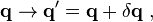
The essence of Noether's theorem is generalizing the ignorable coordinates outlined.

Imagine that the action I defined above is invariant under small perturbations (warpings) of the time variable t and the generalized coordinates q; in a notation commonly used in physics,
t \rightarrow t^{\prime} = t + \delta t
\mathbf{q} \rightarrow \mathbf{q}^{\prime} = \mathbf{q} + \delta \mathbf{q} ~,
where the perturbations δt and δq are both small, but variable. For generality, assume there are (say) N such symmetry transformations of the action, i.e. transformations leaving the action unchanged; labelled by an index r = 1, 2, 3, …, N.

Then the resultant perturbation can be written as a linear sum of the individual types of perturbations,
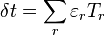
\delta t = \sum_r \varepsilon_r T_r \!
\delta \mathbf{q} = \sum_r \varepsilon_r \mathbf{Q}_r ~,
where εr are infinitesimal parameter coefficients corresponding to each:
For translations, Qr is a constant with units of length; for rotations, it is an expression linear in the components of q, and the parameters make up an angle.

Using these definitions, Noether showed that the N quantities
\left(\frac{\partial L}{\partial \dot{\mathbf{q}}} \cdot \dot{\mathbf{q}} - L \right) T_r - \frac{\partial L}{\partial \dot{\mathbf{q}}} \cdot \mathbf{Q}_r
(which have the dimensions of [energy]·[time] + [momentum]·[length] = [action]) are conserved (constants of motion).

Examples

Time invariance
For illustration, consider a Lagrangian that does not depend on time, i.e., that is invariant (symmetric) under changes tt + δt, without any change in the coordinates q. In this case, N = 1, T = 1 and Q = 0; the corresponding conserved quantity is the total energy H[5]
H = \frac{\partial L}{\partial \dot{\mathbf{q}}} \cdot \dot{\mathbf{q}} - L.
Translational invariance
Consider a Lagrangian which does not depend on an ("ignorable", as above) coordinate qk; so it is invariant (symmetric) under changes qkqk + δqk. In that case, N = 1, T = 0, and Qk = 1; the conserved quantity is the corresponding momentum pk[6]
p_k = \frac{\partial L}{\partial \dot{q_k}}.
In special and general relativity, these apparently separate conservation laws are aspects of a single conservation law, that of the stress–energy tensor,[7] that is derived in the next section.
Rotational invariance
The conservation of the angular momentum L = r × p is analogous to its linear momentum counterpart.[8] It is assumed that the symmetry of the Lagrangian is rotational, i.e., that the Lagrangian does not depend on the absolute orientation of the physical system in space. For concreteness, assume that the Lagrangian does not change under small rotations of an angle δθ about an axis n; such a rotation transforms the Cartesian coordinates by the equation
\mathbf{r} \rightarrow \mathbf{r} + \delta\theta \mathbf{n} \times \mathbf{r}.
Since time is not being transformed, T=0. Taking δθ as the ε parameter and the Cartesian coordinates r as the generalized coordinates q, the corresponding Q variables are given by
\mathbf{Q} = \mathbf{n} \times \mathbf{r}.
Then Noether's theorem states that the following quantity is conserved,

\frac{\partial L}{\partial \dot{\mathbf{q}}} \cdot \mathbf{Q}_{r} = 
\mathbf{p} \cdot \left( \mathbf{n} \times \mathbf{r} \right) = 
\mathbf{n} \cdot \left( \mathbf{r} \times \mathbf{p} \right) = 
\mathbf{n} \cdot \mathbf{L}.
In other words, the component of the angular momentum L along the n axis is conserved.

If n is arbitrary, i.e., if the system is insensitive to any rotation, then every component of L is conserved; in short, angular momentum is conserved.

Field theory version

Although useful in its own right, the version of Noether's theorem just given is a special case of the general version derived in 1915. To give the flavor of the general theorem, a version of the Noether theorem for continuous fields in four-dimensional space–time is now given. Since field theory problems are more common in modern physics than mechanics problems, this field theory version is the most commonly used version (or most often implemented) of Noether's theorem.

Let there be a set of differentiable fields φ defined over all space and time; for example, the temperature T(xt) would be representative of such a field, being a number defined at every place and time. The principle of least action can be applied to such fields, but the action is now an integral over space and time
I = \int L \left(\phi, \partial_\mu \phi, x^\mu \right) \, d^4 x
(the theorem can actually be further generalized to the case where the Lagrangian depends on up to the nth derivative using jet bundles)
Let the action be invariant under certain transformations of the space–time coordinates xμ and the fields φ
x^{\mu} \rightarrow x^\mu + \delta x^\mu \!
\phi \rightarrow\phi + \delta \phi
where the transformations can be indexed by r = 1, 2, 3, …, N
\delta x^\mu = \varepsilon_r X^\mu_r \,
\delta \phi = \varepsilon_r \Psi_r ~.
For such systems, Noether's theorem states that there are N conserved current densities

j^\nu_r = 
- \left( \frac{\partial L}{\partial \phi_{,\nu}} \right) \cdot \Psi_r + 
 \left[ \left( \frac{\partial L}{\partial \phi_{,\nu}} \right) \cdot\phi_{,\sigma} - L \delta^{\nu}_{\sigma} \right] X_{r}^{\sigma}
In such cases, the conservation law is expressed in a four-dimensional way
\partial_{\mu} j^\mu = 0
which expresses the idea that the amount of a conserved quantity within a sphere cannot change unless some of it flows out of the sphere. For example, electric charge is conserved; the amount of charge within a sphere cannot change unless some of the charge leaves the sphere.
For illustration, consider a physical system of fields that behaves the same under translations in time and space, as considered above; in other words, L \left(\boldsymbol\phi, \partial_\mu{\boldsymbol\phi}, x^\mu \right) is constant in its third argument. In that case, N = 4, one for each dimension of space and time. Since only the positions in space–time are being warped, not the fields, the Ψ are all zero and the Xμν equal the Kronecker delta δμν, where we have used μ instead of r for the index. In that case, Noether's theorem corresponds to the conservation law for the stress–energy tensor Tμν[7]

T_\mu{}^\nu =
 \left[ \left( \frac{\partial L}{\partial \phi_{,\nu}} \right) \cdot\phi_{,\sigma} - L\,\delta^\nu_\sigma \right] \delta_\mu^\sigma = 
\left( \frac{\partial L}{\partial\phi_{,\nu}} \right) \cdot\phi_{,\mu} - L\,\delta_\mu^\nu
The conservation of electric charge, by contrast, can be derived by considering zero Xμν=0 and Ψ linear in the fields φ themselves.[9] In quantum mechanics, the probability amplitude ψ(x) of finding a particle at a point x is a complex field φ, because it ascribes a complex number to every point in space and time. The probability amplitude itself is physically unmeasurable; only the probability p = |ψ|2 can be inferred from a set of measurements. Therefore, the system is invariant under transformations of the ψ field and its complex conjugate field ψ* that leave |ψ|2 unchanged, such as
\psi \rightarrow e^{i\theta} \psi \ ,\ \psi^{*} \rightarrow e^{-i\theta} \psi^{*}~,
a complex rotation. In the limit when the phase θ becomes infinitesimally small, δθ, it may be taken as the parameter ε, while the Ψ are equal to and −*, respectively. A specific example is the Klein–Gordon equation, the relativistically correct version of the Schrödinger equation for spinless particles, which has the Lagrangian density
L = \psi_{,\nu} \psi^{*}_{,\mu} \eta^{\nu \mu} + m^2 \psi \psi^{*}.
In this case, Noether's theorem states that the conserved (∂⋅j = 0) current equals
j^{\nu} = i \left( \frac{\partial \psi}{\partial x^{\mu}} \psi^{*} - \frac{\partial \psi^{*}}{\partial x^{\mu}} \psi \right) \eta^{\nu \mu}~,
which, when multiplied by the charge on that species of particle, equals the electric current density due to that type of particle. This "gauge invariance" was first noted by Hermann Weyl, and is one of the prototype gauge symmetries of physics.

Derivations

One independent variable

Consider the simplest case, a system with one independent variable, time. Suppose the dependent variables q are such that the action integral
I = \int_{t_1}^{t_2} L [\mathbf{q} [t], \dot{\mathbf{q}} [t], t] \, dt
is invariant under brief infinitesimal variations in the dependent variables. In other words, they satisfy the Euler–Lagrange equations
\frac{d}{dt} \frac{\partial L}{\partial \dot{\mathbf{q}}} [t] = \frac{\partial L}{\partial \mathbf{q}} [t].
And suppose that the integral is invariant under a continuous symmetry. Mathematically such a symmetry is represented as a flow, φ, which acts on the variables as follows
t \rightarrow t' = t + \varepsilon T \!
\mathbf{q} [t] \rightarrow \mathbf{q}' [t'] = \phi [\mathbf{q} [t], \varepsilon] = \phi [\mathbf{q} [t' - \varepsilon T], \varepsilon]
where ε is a real variable indicating the amount of flow, and T is a real constant (which could be zero) indicating how much the flow shifts time.

\dot{\mathbf{q}} [t] \rightarrow \dot{\mathbf{q}}' [t'] = \frac{d}{dt} \phi [\mathbf{q} [t], \varepsilon] = \frac{\partial \phi}{\partial \mathbf{q}} [\mathbf{q} [t' - \varepsilon T], \varepsilon] \dot{\mathbf{q}} [t' - \varepsilon T]
.
The action integral flows to

\begin{align}
I' [\varepsilon] & = \int_{t_1 + \varepsilon T}^{t_2 + \varepsilon T} L [\mathbf{q}'[t'], \dot{\mathbf{q}}' [t'], t'] \, dt' \\[6pt]
& = \int_{t_1 + \varepsilon T}^{t_2 + \varepsilon T} L [\phi [\mathbf{q} [t' - \varepsilon T], \varepsilon], \frac{\partial \phi}{\partial \mathbf{q}} [\mathbf{q} [t' - \varepsilon T], \varepsilon] \dot{\mathbf{q}} [t' - \varepsilon T], t'] \, dt'
\end{align}
which may be regarded as a function of ε. Calculating the derivative at ε = 0 and using the symmetry, we get

\begin{align}
0 & = \frac{d I'}{d \varepsilon} [0] = L [\mathbf{q} [t_2], \dot{\mathbf{q}} [t_2], t_2] T - L [\mathbf{q} [t_1], \dot{\mathbf{q}} [t_1], t_1] T \\[6pt]
& {} + \int_{t_1}^{t_2} \frac{\partial L}{\partial \mathbf{q}} \left( - \frac{\partial \phi}{\partial \mathbf{q}} \dot{\mathbf{q}} T + \frac{\partial \phi}{\partial \varepsilon} \right) + \frac{\partial L}{\partial \dot{\mathbf{q}}} \left( - \frac{\partial^2 \phi}{(\partial \mathbf{q})^2} {\dot{\mathbf{q}}}^2 T + \frac{\partial^2 \phi}{\partial \varepsilon \partial \mathbf{q}} \dot{\mathbf{q}} -
\frac{\partial \phi}{\partial \mathbf{q}} \ddot{\mathbf{q}} T \right) \, dt.
\end{align}
Notice that the Euler–Lagrange equations imply

\begin{align}
\frac{d}{dt} \left( \frac{\partial L}{\partial \dot{\mathbf{q}}} \frac{\partial \phi}{\partial \mathbf{q}} \dot{\mathbf{q}} T \right) 
& = \left( \frac{d}{dt} \frac{\partial L}{\partial \dot{\mathbf{q}}} \right) \frac{\partial \phi}{\partial \mathbf{q}} \dot{\mathbf{q}} T + \frac{\partial L}{\partial \dot{\mathbf{q}}} \left( \frac{d}{dt} \frac{\partial \phi}{\partial \mathbf{q}} \right) \dot{\mathbf{q}} T + \frac{\partial L}{\partial \dot{\mathbf{q}}} \frac{\partial \phi}{\partial \mathbf{q}} \ddot{\mathbf{q}} \, T \\[6pt]
& = \frac{\partial L}{\partial \mathbf{q}} \frac{\partial \phi}{\partial \mathbf{q}} \dot{\mathbf{q}} T + \frac{\partial L}{\partial \dot{\mathbf{q}}} \left( \frac{\partial^2 \phi}{(\partial \mathbf{q})^2} \dot{\mathbf{q}} \right) \dot{\mathbf{q}} T + \frac{\partial L}{\partial \dot{\mathbf{q}}} \frac{\partial \phi}{\partial \mathbf{q}} \ddot{\mathbf{q}} \, T.
\end{align}
Substituting this into the previous equation, one gets

\begin{align}
0 & = \frac{d I'}{d \varepsilon} [0] = L [\mathbf{q} [t_2], \dot{\mathbf{q}} [t_2], t_2] T - L [\mathbf{q} [t_1], \dot{\mathbf{q}} [t_1], t_1] T - \frac{\partial L}{\partial \dot{\mathbf{q}}} \frac{\partial \phi}{\partial \mathbf{q}} \dot{\mathbf{q}} [t_2] T + \frac{\partial L}{\partial \dot{\mathbf{q}}} \frac{\partial \phi}{\partial \mathbf{q}} \dot{\mathbf{q}} [t_1] T \\[6pt]
& {} + \int_{t_1}^{t_2} \frac{\partial L}{\partial \mathbf{q}} \frac{\partial \phi}{\partial \varepsilon} + \frac{\partial L}{\partial \dot{\mathbf{q}}} \frac{\partial^2 \phi}{\partial \varepsilon \partial \mathbf{q}} \dot{\mathbf{q}} \, dt.
\end{align}
Again using the Euler–Lagrange equations we get

\frac{d}{d t} \left( \frac{\partial L}{\partial \dot{\mathbf{q}}} \frac{\partial \phi}{\partial \varepsilon} \right) 
= \left( \frac{d}{d t} \frac{\partial L}{\partial \dot{\mathbf{q}}} \right) \frac{\partial \phi}{\partial \varepsilon} + \frac{\partial L}{\partial \dot{\mathbf{q}}} \frac{\partial^2 \phi}{\partial \varepsilon \partial \mathbf{q}} \dot{\mathbf{q}}
= \frac{\partial L}{\partial \mathbf{q}} \frac{\partial \phi}{\partial \varepsilon} + \frac{\partial L}{\partial \dot{\mathbf{q}}} \frac{\partial^2 \phi}{\partial \varepsilon \partial \mathbf{q}} \dot{\mathbf{q}}.
Substituting this into the previous equation, one gets

\begin{align}
0 & = L [\mathbf{q} [t_2], \dot{\mathbf{q}} [t_2], t_2] T - L [\mathbf{q} [t_1], \dot{\mathbf{q}} [t_1], t_1] T - \frac{\partial L}{\partial \dot{\mathbf{q}}} \frac{\partial \phi}{\partial \mathbf{q}} \dot{\mathbf{q}} [t_2] T + \frac{\partial L}{\partial \dot{\mathbf{q}}} \frac{\partial \phi}{\partial \mathbf{q}} \dot{\mathbf{q}} [t_1] T \\[6pt]
& {} + \frac{\partial L}{\partial \dot{\mathbf{q}}} \frac{\partial \phi}{\partial \varepsilon} [t_2] - \frac{\partial L}{\partial \dot{\mathbf{q}}} \frac{\partial \phi}{\partial \varepsilon} [t_1].
\end{align}
From which one can see that
\left( \frac{\partial L}{\partial \dot{\mathbf{q}}} \frac{\partial \phi}{\partial \mathbf{q}} \dot{\mathbf{q}} - L \right) T - \frac{\partial L}{\partial \dot{\mathbf{q}}} \frac{\partial \phi}{\partial \varepsilon}
is a constant of the motion, i.e., it is a conserved quantity. Since φ[q, 0] = q, we get \frac{\partial \phi}{\partial \mathbf{q}} = 1 and so the conserved quantity simplifies to
\left( \frac{\partial L}{\partial \dot{\mathbf{q}}} \dot{\mathbf{q}} - L \right) T - \frac{\partial L}{\partial \dot{\mathbf{q}}} \frac{\partial \phi}{\partial \varepsilon}.
To avoid excessive complication of the formulas, this derivation assumed that the flow does not change as time passes. The same result can be obtained in the more general case.

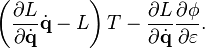
Field-theoretic derivation

Noether's theorem may also be derived for tensor fields φA where the index A ranges over the various components of the various tensor fields. These field quantities are functions defined over a four-dimensional space whose points are labeled by coordinates xμ where the index μ ranges over time (μ = 0) and three spatial dimensions (μ = 1, 2, 3). These four coordinates are the independent variables; and the values of the fields at each event are the dependent variables. Under an infinitesimal transformation, the variation in the coordinates is written
x^\mu \rightarrow \xi^\mu = x^\mu + \delta x^\mu \!
whereas the transformation of the field variables is expressed as
\phi^A \rightarrow \alpha^A (\xi^\mu) = \phi^A (x^\mu) + \delta \phi^A (x^\mu)\,.
By this definition, the field variations δφA result from two factors: intrinsic changes in the field themselves and changes in coordinates, since the transformed field αA depends on the transformed coordinates ξμ. To isolate the intrinsic changes, the field variation at a single point xμ may be defined
\alpha^A (x^\mu) = \phi^A (x^\mu) + \bar{\delta} \phi^A (x^\mu)\,.
If the coordinates are changed, the boundary of the region of space–time over which the Lagrangian is being integrated also changes; the original boundary and its transformed version are denoted as Ω and Ω’, respectively.
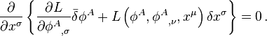
Noether's theorem begins with the assumption that a specific transformation of the coordinates and field variables does not change the action, which is defined as the integral of the Lagrangian density over the given region of spacetime. Expressed mathematically, this assumption may be written as
\int_{\Omega^{\prime}} L \left( \alpha^A, {\alpha^A}_{,\nu}, \xi^{\mu} \right) d^{4}\xi - \int_{\Omega} L \left( \phi^A, {\phi^A}_{,\nu}, x^{\mu} \right) d^{4}x = 0
where the comma subscript indicates a partial derivative with respect to the coordinate(s) that follows the comma, e.g.
{\phi^A}_{,\sigma} = \frac{\partial \phi^A}{\partial x^{\sigma}}\,.
Since ξ is a dummy variable of integration, and since the change in the boundary Ω is infinitesimal by assumption, the two integrals may be combined using the four-dimensional version of the divergence theorem into the following form

\int_{\Omega} \left\{ 
\left[ L \left( \alpha^A, {\alpha^A}_{,\nu}, x^\mu \right) - 
L \left( \phi^A, {\phi^A}_{,\nu}, x^\mu \right) \right]
+ \frac{\partial}{\partial x^\sigma} \left[ L \left( \phi^A, {\phi^A}_{,\nu}, x^\mu \right) \delta x^\sigma \right]
\right\} d^4 x = 0
\,.
The difference in Lagrangians can be written to first-order in the infinitesimal variations as

\left[ L \left( \alpha^A, {\alpha^A}_{,\nu}, x^\mu \right) - 
L \left( \phi^A, {\phi^A}_{,\nu}, x^\mu \right) \right] = 
\frac{\partial L}{\partial \phi^A} \bar{\delta} \phi^A + 
\frac{\partial L}{\partial {\phi^A}_{,\sigma}} \bar{\delta} {\phi^A}_{,\sigma}
\,.
However, because the variations are defined at the same point as described above, the variation and the derivative can be done in reverse order; they commute

\bar{\delta} {\phi^A}_{,\sigma} = 
\bar{\delta} \frac{\partial \phi^A}{\partial x^\sigma} = 
\frac{\partial}{\partial x^\sigma} ( \bar{\delta} \phi^A)
\,.
Using the Euler–Lagrange field equations

\frac{\partial}{\partial x^\sigma} \left( \frac{\partial L}{\partial {\phi^A}_{,\sigma}} \right) =
\frac{\partial L}{\partial \phi^A}
the difference in Lagrangians can be written neatly as

\left[ L \left( \alpha^A, {\alpha^A}_{,\nu}, x^\mu \right) - 
L \left( \phi^A, {\phi^A}_{,\nu}, x^{\mu} \right) \right] 
= \frac{\partial}{\partial x^\sigma} \left( \frac{\partial L}{\partial {\phi^A}_{,\sigma}} \right) \bar{\delta} \phi^A + 
\frac{\partial L}{\partial {\phi^A}_{,\sigma}} \bar{\delta} {\phi^A}_{,\sigma}
= \frac{\partial}{\partial x^\sigma} 
\left( \frac{\partial L}{\partial {\phi^A}_{,\sigma}} \bar{\delta} \phi^A \right)
\,.
Thus, the change in the action can be written as

\int_\Omega \frac{\partial}{\partial x^\sigma} 
\left\{ \frac{\partial L}{\partial {\phi^A}_{,\sigma}} \bar{\delta} \phi^A + 
L \left( \phi^A, {\phi^A}_{,\nu}, x^\mu \right) \delta x^\sigma
\right\} d^{4}x = 0
\,.
Since this holds for any region Ω, the integrand must be zero

\frac{\partial}{\partial x^\sigma} 
\left\{ \frac{\partial L}{\partial {\phi^A}_{,\sigma}} \bar{\delta} \phi^A + 
L \left( \phi^A, {\phi^A}_{,\nu}, x^\mu \right) \delta x^\sigma
\right\} = 0
\,.
For any combination of the various symmetry transformations, the perturbation can be written
\delta x^{\mu} = \varepsilon X^\mu\!
\delta \phi^A = \varepsilon \Psi^A = \bar{\delta} \phi^A + \varepsilon \mathcal{L}_X \phi^A
where \mathcal{L}_X \phi^A is the Lie derivative of φA in the Xμ direction. When φA is a scalar or {X^\mu}_{,\nu} = 0 \,,
\mathcal{L}_X \phi^A = \frac{\partial \phi^A}{\partial x^{\mu}} X^\mu\,.
These equations imply that the field variation taken at one point equals
\bar{\delta} \phi^A = \varepsilon \Psi^A - \varepsilon \mathcal{L}_X \phi^A\,.
Differentiating the above divergence with respect to ε at ε=0 and changing the sign yields the conservation law
\frac{\partial }{\partial x^\sigma} j^\sigma = 0
where the conserved current equals

j^\sigma = 
\left[\frac{\partial L}{\partial {\phi^A}_{,\sigma}} \mathcal{L}_X \phi^A - L \, X^\sigma\right]
- \left(\frac{\partial L}{\partial {\phi^A}_{,\sigma}} \right) \Psi^A\,.

Manifold/fiber bundle derivation

Suppose we have an n-dimensional oriented Riemannian manifold, M and a target manifold T. Let \mathcal{C} be the configuration space of smooth functions from M to T. (More generally, we can have smooth sections of a fiber bundle over M.)

Examples of this M in physics include:
Now suppose there is a functional
\mathcal{S}:\mathcal{C}\rightarrow \mathbf{R},
called the action. (Note that it takes values into R, rather than C; this is for physical reasons, and doesn't really matter for this proof.)
To get to the usual version of Noether's theorem, we need additional restrictions on the action. We assume \mathcal{S}[\phi] is the integral over M of a function
\mathcal{L}(\phi,\partial_\mu\phi,x)
called the Lagrangian density, depending on φ, its derivative and the position. In other words, for φ in \mathcal{C}
 \mathcal{S}[\phi]\,=\,\int_M \mathcal{L}[\phi(x),\partial_\mu\phi(x),x] \mathrm{d}^nx.
Suppose we are given boundary conditions, i.e., a specification of the value of φ at the boundary if M is compact, or some limit on φ as x approaches ∞. Then the subspace of \mathcal{C} consisting of functions φ such that all functional derivatives of \mathcal{S} at φ are zero, that is:
\frac{\delta \mathcal{S}[\phi]}{\delta \phi(x)}\approx 0
and that φ satisfies the given boundary conditions, is the subspace of on shell solutions. (See principle of stationary action)

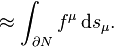
Now, suppose we have an infinitesimal transformation on \mathcal{C}, generated by a functional derivation, Q such that
Q \left[ \int_N \mathcal{L} \, \mathrm{d}^n x \right] \approx \int_{\partial N} f^\mu [\phi(x),\partial\phi,\partial\partial\phi,\ldots] \, \mathrm{d}s_\mu
for all compact submanifolds N or in other words,
Q[\mathcal{L}(x)]\approx\partial_\mu f^\mu(x)
for all x, where we set
\mathcal{L}(x)=\mathcal{L}[\phi(x), \partial_\mu \phi(x),x].\
If this holds on shell and off shell, we say Q generates an off-shell symmetry. If this only holds on shell, we say Q generates an on-shell symmetry. Then, we say Q is a generator of a one parameter symmetry Lie group.

Now, for any N, because of the Euler–Lagrange theorem, on shell (and only on-shell), we have
Q\left[\int_N \mathcal{L} \, \mathrm{d}^nx \right] =\int_N \left[\frac{\partial\mathcal{L}}{\partial\phi}-
\partial_\mu\frac{\partial\mathcal{L}}{\partial(\partial_\mu\phi)}\right]Q[\phi] \, \mathrm{d}^nx +
\int_{\partial N} \frac{\partial\mathcal{L}}{\partial(\partial_\mu\phi)}Q[\phi] \, \mathrm{d}s_\mu
\approx\int_{\partial N} f^\mu \, \mathrm{d}s_\mu .
Since this is true for any N, we have
\partial_\mu\left[\frac{\partial\mathcal{L}}{\partial(\partial_\mu\phi)}Q[\phi]-f^\mu\right]\approx 0.
But this is the continuity equation for the current J^\mu\,\! defined by:[10]
J^\mu\,=\,\frac{\partial\mathcal{L}}{\partial(\partial_\mu\phi)}Q[\phi]-f^\mu,
which is called the Noether current associated with the symmetry. The continuity equation tells us that if we integrate this current over a space-like slice, we get a conserved quantity called the Noether charge (provided, of course, if M is noncompact, the currents fall off sufficiently fast at infinity).

Comments

Noether's theorem is an on shell theorem: it relies on use of the equations of motion—the classical path. It reflects the relation between the boundary conditions and the variational principle. Assuming no boundary terms in the action, Noether's theorem implies that
\int_{\partial N} J^\mu \mathrm{d}s_\mu \approx 0~.
The quantum analogs of Noether's theorem involving expectation values, e.g. ⟨∫d4x ∂·J⟩ = 0, probing off shell quantities as well are the Ward–Takahashi identities.

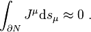
Generalization to Lie algebras

Suppose say we have two symmetry derivations Q1 and Q2. Then, [Q1Q2] is also a symmetry derivation. Let's see this explicitly. Let's say
Q_1[\mathcal{L}]\approx\partial_\mu f_1^\mu
and
Q_2[\mathcal{L}]\approx\partial_\mu f_2^\mu
Then,
[Q_1,Q_2][\mathcal{L}]=Q_1[Q_2[\mathcal{L}]]-Q_2[Q_1[\mathcal{L}]]\approx\partial_\mu f_{12}^\mu
where f12 = Q1[f2μ] − Q2[f1μ]. So,
j_{12}^\mu=\left(\frac{\partial}{\partial (\partial_\mu\phi)}\mathcal{L}\right)(Q_1[Q_2[\phi]]-Q_2[Q_1[\phi]])-f_{12}^\mu.
This shows we can extend Noether's theorem to larger Lie algebras in a natural way.

Generalization of the proof

This applies to any local symmetry derivation Q satisfying QS ≈ 0, and also to more general local functional differentiable actions, including ones where the Lagrangian depends on higher derivatives of the fields. Let ε be any arbitrary smooth function of the spacetime (or time) manifold such that the closure of its support is disjoint from the boundary. ε is a test function. Then, because of the variational principle (which does not apply to the boundary, by the way), the derivation distribution q generated by q[ε][Φ(x)] = ε(x)Q[Φ(x)] satisfies q[ε][S] ≈ 0 for every ε, or more compactly, q(x)[S] ≈ 0 for all x not on the boundary (but remember that q(x) is a shorthand for a derivation distribution, not a derivation parametrized by x in general). This is the generalization of Noether's theorem.
To see how the generalization is related to the version given above, assume that the action is the spacetime integral of a Lagrangian that only depends on φ and its first derivatives. Also, assume
Q[\mathcal{L}]\approx\partial_\mu f^\mu
Then,

\begin{align}
q[\varepsilon][\mathcal{S}] & = \int q[\varepsilon][\mathcal{L}] \, \mathrm{d}^n x  \\
& = \int \left\{ \left(\frac{\partial}{\partial \phi}\mathcal{L}\right) \varepsilon Q[\phi]+ \left[\frac{\partial}{\partial (\partial_\mu \phi)}\mathcal{L}\right]\partial_\mu(\varepsilon Q[\phi]) \right\} \, \mathrm{d}^n x \\
& = \int \left\{ \varepsilon Q[\mathcal{L}] + \partial_{\mu}\varepsilon \left[\frac{\partial}{\partial \left( \partial_\mu \phi\right)} \mathcal{L} \right] Q[\phi] \right\} \, \mathrm{d}^n x \\
& \approx \int \varepsilon \partial_\mu \left\{f^\mu-\left[\frac{\partial}{\partial (\partial_\mu\phi)}\mathcal{L}\right]Q[\phi]\right\} \, \mathrm{d}^n x
\end{align}
for all ε.

More generally, if the Lagrangian depends on higher derivatives, then
\partial_\mu\left[f^\mu-\left[\frac{\partial}{\partial (\partial_\mu\phi)} \mathcal{L} \right] Q[\phi] - 2\left[\frac{\partial}{\partial (\partial_\mu \partial_\nu \phi)}\mathcal{L}\right]\partial_\nu Q[\phi]+\partial_\nu\left[\left[\frac{\partial}{\partial (\partial_\mu \partial_\nu \phi)}\mathcal{L}\right] Q[\phi]\right]-\,\cdots\right]\approx 0.

Examples

Example 1: Conservation of energy

Looking at the specific case of a Newtonian particle of mass m, coordinate x, moving under the influence of a potential V, coordinatized by time t. The action, S, is:

\begin{align}
\mathcal{S}[x] & = \int L[x(t),\dot{x}(t)] \, dt \\
& = \int \left(\frac{m}{2}\sum_{i=1}^3\dot{x}_i^2-V(x(t))\right) \, dt.
\end{align}
The first term in the brackets is the kinetic energy of the particle, whilst the second is its potential energy. Consider the generator of time translations Q = ∂/∂t. In other words, Q[x(t)]=\dot{x}(t). Note that x has an explicit dependence on time, whilst V does not; consequently:
Q[L]=m \sum_i\dot{x}_i\ddot{x}_i-\sum_i\frac{\partial V(x)}{\partial x_i}\dot{x}_i = \frac{d}{dt}\left[\frac{m}{2}\sum_i\dot{x}_i^2-V(x)\right]
so we can set
f=\frac{m}{2} \sum_i\dot{x}_i^2-V(x).
Then,

\begin{align}
j & = \sum_{i=1}^3\frac{\partial L}{\partial \dot{x}_i}Q[x_i]-f \\
& = m \sum_i\dot{x}_i^2 -\left[\frac{m}{2}\sum_i\dot{x}_i^2 -V(x)\right] \\
& = \frac{m}{2}\sum_i\dot{x}_i^2+V(x).
\end{align}
The right hand side is the energy, and Noether's theorem states that \dot{j}=0 (i.e. the principle of conservation of energy is a consequence of invariance under time translations).

More generally, if the Lagrangian does not depend explicitly on time, the quantity
\sum_{i=1}^3 \frac{\partial L}{\partial \dot{x}_i}\dot{x_i}-L
(called the Hamiltonian) is conserved.

Example 2: Conservation of center of momentum

Still considering 1-dimensional time, let

\begin{align}
\mathcal{S}[\vec{x}] & = \int \mathcal{L}[\vec{x}(t),\dot{\vec{x}}(t)] \, \mathrm{d}t \\
& = \int \left [\sum^N_{\alpha=1} \frac{m_\alpha}{2}(\dot{\vec{x}}_\alpha)^2 -\sum_{\alpha<\beta} V_{\alpha\beta}(\vec{x}_\beta-\vec{x}_\alpha)\right] \, \mathrm{d}t
\end{align}
i.e. N Newtonian particles where the potential only depends pairwise upon the relative displacement.
For \vec{Q}, let's consider the generator of Galilean transformations (i.e. a change in the frame of reference). In other words,
Q_i[x^j_\alpha(t)]=t \delta^j_i. \,
Note that

\begin{align}
Q_i[\mathcal{L}] & = \sum_\alpha m_\alpha \dot{x}_\alpha^i-\sum_{\alpha<\beta}\partial_i V_{\alpha\beta}(\vec{x}_\beta-\vec{x}_\alpha)(t-t) \\
& = \sum_\alpha m_\alpha \dot{x}_\alpha^i.
\end{align}
This has the form of \frac{\mathrm{d}}{\mathrm{d}t}\sum_\alpha m_\alpha x^i_\alpha so we can set
\vec{f}=\sum_\alpha m_\alpha \vec{x}_\alpha.
Then,
\vec{j}=\sum_\alpha \left(\frac{\partial}{\partial \dot{\vec{x}}_\alpha}\mathcal{L}\right)\cdot\vec{Q}[\vec{x}_\alpha]-\vec{f}
=\sum_\alpha (m_\alpha \dot{\vec{x}}_\alpha t-m_\alpha \vec{x}_\alpha)
=\vec{P}t-M\vec{x}_{CM}
where \vec{P} is the total momentum, M is the total mass and \vec{x}_{CM} is the center of mass. Noether's theorem states:
\dot{\vec{j}} = 0 \Rightarrow {\vec{P}}-M \dot{\vec{x}}_{CM} = 0.

Example 3: Conformal transformation

Both examples 1 and 2 are over a 1-dimensional manifold (time). An example involving spacetime is a conformal transformation of a massless real scalar field with a quartic potential in (3 + 1)-Minkowski spacetime.
\mathcal{S}[\phi]\, =\int \mathcal{L}[\phi (x),\partial_\mu \phi (x)] \, \mathrm{d}^4x
=\int \left( \frac{1}{2}\partial^\mu \phi \partial_\mu \phi -\lambda \phi^4\right ) \, \mathrm{d}^4x
For Q, consider the generator of a spacetime rescaling. In other words,
Q[\phi(x)]=x^\mu\partial_\mu \phi(x)+\phi(x). \!
The second term on the right hand side is due to the "conformal weight" of φ. Note that
Q[\mathcal{L}]=\partial^\mu\phi\left(\partial_\mu\phi+x^\nu\partial_\mu\partial_\nu\phi+\partial_\mu\phi\right)-4\lambda\phi^3\left(x^\mu\partial_\mu\phi+\phi\right).
This has the form of
\partial_\mu\left[\frac{1}{2}x^\mu\partial^\nu\phi\partial_\nu\phi-\lambda x^\mu \phi^4 \right] = \partial_\mu\left(x^\mu\mathcal{L}\right)
(where we have performed a change of dummy indices) so set
f^\mu=x^\mu\mathcal{L}.\,
Then,
j^\mu=\left[\frac{\partial}{\partial
(\partial_\mu\phi)}\mathcal{L}\right]Q[\phi]-f^\mu
=\partial^\mu\phi\left(x^\nu\partial_\nu\phi+\phi\right)-x^\mu\left(\frac{1}{2}\partial^\nu\phi\partial_\nu\phi-\lambda\phi^4\right).
Noether's theorem states that \partial_\mu j^\mu = 0 \! (as one may explicitly check by substituting the Euler–Lagrange equations into the left hand side).

(Aside: If one tries to find the Ward–Takahashi analog of this equation, one runs into a problem because of anomalies.)

Applications

Application of Noether's theorem allows physicists to gain powerful insights into any general theory in physics, by just analyzing the various transformations that would make the form of the laws involved invariant. For example:
In quantum field theory, the analog to Noether's theorem, the Ward–Takahashi identity, yields further conservation laws, such as the conservation of electric charge from the invariance with respect to a change in the phase factor of the complex field of the charged particle and the associated gauge of the electric potential and vector potential.

The Noether charge is also used in calculating the entropy of stationary black holes.[11]
More climate change chicanery.  The graph above (which I gleaned from Noah Diffenbaugh's Google posts), is an attempt to make climate prediction inaccuracies vanish.  The light, pointed line is actual global temperatures from 2000 - 2012.  As it is fresh data, they are the real global temperatures, from satellites and ground stations; little or no adjustments needed.  The dotted lines are some several (not all) model projections, with the shaded uncertainty of them in the blue band (note how this band keeps growing wider in time).

The years 1970-1990 are all in good agreement, though how they match earlier is unknown from this graph.

What is the red line?  It is the result of taking the real data, and removing all factors (el nino years, volcanism, alleged or real, etc.); that is, removing all factors not accounted for in the models. Of course the agreement is good; the red line is being forced to cover only what the models cover; by definition, agreement must be excellent.  This is what is known in logical as circular reasoning.  We know the models be correct, ergo the data must fit it.

In reality. the actual data reach a peak in 1998 (an El Nino year), and, on average, proceeds pretty horizontally to the end of the data (the hiatus), while the models keep predicting ever rising temperatures.

What's especially interesting here is that critics will and have cried "foul" at the inclusion of the '98 El Nino, but have freely used the 2014-2015 (and maybe into 2016), to imply that overall warming has started again -- though, by their own analysis, they must be adjusted out of the real data.

What this all demonstrates is that current models cannot predict real world data out to a decade or two, and yet we're supposed to believe them out to 2100.  And new data, requiring readjustments every years (plus old ones, like clouds, which still aren't well understand), shouldn't dent our faith one millimeter.

I won't draw any conclusions.  I think they're obvious.


Lie group


From Wikipedia, the free encyclopedia

In mathematics, a Lie group /ˈl/ is a group that is also a differentiable manifold, with the property that the group operations are compatible with the smooth structure. Lie groups are named after Sophus Lie, who laid the foundations of the theory of continuous transformation groups. The term groupes de Lie first appeared in French in 1893 in the thesis of Lie’s student Arthur Tresse, page 3.[1]

Lie groups represent the best-developed theory of continuous symmetry of mathematical objects and structures, which makes them indispensable tools for many parts of contemporary mathematics, as well as for modern theoretical physics. They provide a natural framework for analysing the continuous symmetries of differential equations (differential Galois theory), in much the same way as permutation groups are used in Galois theory for analysing the discrete symmetries of algebraic equations. An extension of Galois theory to the case of continuous symmetry groups was one of Lie's principal motivations.

Overview


The circle of center 0 and radius 1 in the complex plane is a Lie group with complex multiplication.

Lie groups are smooth[Note 1] differentiable manifolds and as such can be studied using differential calculus, in contrast with the case of more general topological groups. One of the key ideas in the theory of Lie groups is to replace the global object, the group, with its local or linearized version, which Lie himself called its "infinitesimal group" and which has since become known as its Lie algebra.

Lie groups play an enormous role in modern geometry, on several different levels. Felix Klein argued in his Erlangen program that one can consider various "geometries" by specifying an appropriate transformation group that leaves certain geometric properties invariant. Thus Euclidean geometry corresponds to the choice of the group E(3) of distance-preserving transformations of the Euclidean space R3, conformal geometry corresponds to enlarging the group to the conformal group, whereas in projective geometry one is interested in the properties invariant under the projective group. This idea later led to the notion of a G-structure, where G is a Lie group of "local" symmetries of a manifold. On a "global" level, whenever a Lie group acts on a geometric object, such as a Riemannian or a symplectic manifold, this action provides a measure of rigidity and yields a rich algebraic structure. The presence of continuous symmetries expressed via a Lie group action on a manifold places strong constraints on its geometry and facilitates analysis on the manifold. Linear actions of Lie groups are especially important, and are studied in representation theory.

In the 1940s–1950s, Ellis Kolchin, Armand Borel, and Claude Chevalley realised that many foundational results concerning Lie groups can be developed completely algebraically, giving rise to the theory of algebraic groups defined over an arbitrary field. This insight opened new possibilities in pure algebra, by providing a uniform construction for most finite simple groups, as well as in algebraic geometry. The theory of automorphic forms, an important branch of modern number theory, deals extensively with analogues of Lie groups over adele rings; p-adic
Lie groups play an important role, via their connections with Galois representations in number theory.

Definitions and examples

A real Lie group is a group that is also a finite-dimensional real smooth manifold, in which the group operations of multiplication and inversion are smooth maps. Smoothness of the group multiplication
 \mu:G\times G\to G\quad \mu(x,y)=xy
means that μ is a smooth mapping of the product manifold G×G into G. These two requirements can be combined to the single requirement that the mapping
(x,y)\mapsto x^{-1}y
be a smooth mapping of the product manifold into G.

First examples

 \operatorname{GL}(2, \mathbf{R}) = \left\{A=\begin{pmatrix}a&b\\c&d\end{pmatrix}: \det A=ad-bc \ne 0\right\}.
This is a four-dimensional noncompact real Lie group. This group is disconnected; it has two connected components corresponding to the positive and negative values of the determinant.
  • The rotation matrices form a subgroup of GL(2, R), denoted by SO(2, R). It is a Lie group in its own right: specifically, a one-dimensional compact connected Lie group which is diffeomorphic to the circle. Using the rotation angle \varphi as a parameter, this group can be parametrized as follows:
 \operatorname{SO}(2, \mathbf{R}) =\left\{\begin{pmatrix} \cos\varphi & -\sin \varphi \\ \sin \varphi & \cos \varphi \end{pmatrix}:  \varphi\in\mathbf{R}/2\pi\mathbf{Z}\right\}.
Addition of the angles corresponds to multiplication of the elements of SO(2, R), and taking the opposite angle corresponds to inversion. Thus both multiplication and inversion are differentiable maps.
All of the previous examples of Lie groups fall within the class of classical groups.

Related concepts

A complex Lie group is defined in the same way using complex manifolds rather than real ones (example: SL(2, C)), and similarly, using an alternate metric completion of Q, one can define a p-adic Lie group over the p-adic numbers, a topological group in which each point has a p-adic neighborhood. Hilbert's fifth problem asked whether replacing differentiable manifolds with topological or analytic ones can yield new examples. The answer to this question turned out to be negative: in 1952, Gleason, Montgomery and Zippin showed that if G is a topological manifold with continuous group operations, then there exists exactly one analytic structure on G which turns it into a Lie group (see also Hilbert–Smith conjecture). If the underlying manifold is allowed to be infinite-dimensional (for example, a Hilbert manifold), then one arrives at the notion of an infinite-dimensional Lie group. It is possible to define analogues of many Lie groups over finite fields, and these give most of the examples of finite simple groups.

The language of category theory provides a concise definition for Lie groups: a Lie group is a group object in the category of smooth manifolds. This is important, because it allows generalization of the notion of a Lie group to Lie supergroups.

More examples of Lie groups

Lie groups occur in abundance throughout mathematics and physics. Matrix groups or algebraic groups are (roughly) groups of matrices (for example, orthogonal and symplectic groups), and these give most of the more common examples of Lie groups.

Examples with a specific number of dimensions

  • The circle group S1 consisting of angles mod 2π under addition or, alternatively, the complex numbers with absolute value 1 under multiplication. This is a one-dimensional compact connected abelian Lie group.
  • The 3-sphere S3 forms a Lie group by identification with the set of quaternions of unit norm, called versors. The only other spheres that admit the structure of a Lie group are the 0-sphere S0 (real numbers with absolute value 1) and the circle S1 (complex numbers with absolute value 1). For example, for even n > 1, Sn is not a Lie group because it does not admit a nonvanishing vector field and so a fortiori cannot be parallelizable as a differentiable manifold. Of the spheres only S0, S1, S3, and S7 are parallelizable. The last carries the structure of a Lie quasigroup (a nonassociative group), which can be identified with the set of unit octonions.
  • The (3-dimensional) metaplectic group is a double cover of SL(2, R) playing an important role in the theory of modular forms. It is a connected Lie group that cannot be faithfully represented by matrices of finite size, i.e., a nonlinear group.
  • The Heisenberg group is a connected nilpotent Lie group of dimension 3, playing a key role in quantum mechanics.
  • The Lorentz group is a 6-dimensional Lie group of linear isometries of the Minkowski space.
  • The Poincaré group is a 10-dimensional Lie group of affine isometries of the Minkowski space.
  • The group U(1)×SU(2)×SU(3) is a Lie group of dimension 1+3+8=12 that is the gauge group of the Standard Model in particle physics. The dimensions of the factors correspond to the 1 photon + 3 vector bosons + 8 gluons of the standard model
  • The exceptional Lie groups of types G2, F4, E6, E7, E8 have dimensions 14, 52, 78, 133, and 248. Along with the A-B-C-D series of simple Lie groups, the exceptional groups complete the list of simple Lie groups. There is also a Lie group named E of dimension 190, but it is not a simple Lie group.

Examples with n dimensions

Constructions

There are several standard ways to form new Lie groups from old ones:
  • The product of two Lie groups is a Lie group.
  • Any topologically closed subgroup of a Lie group is a Lie group. This is known as the Closed subgroup theorem or Cartan's theorem.
  • The quotient of a Lie group by a closed normal subgroup is a Lie group.
  • The universal cover of a connected Lie group is a Lie group. For example, the group R is the universal cover of the circle group S1. In fact any covering of a differentiable manifold is also a differentiable manifold, but by specifying universal cover, one guarantees a group structure (compatible with its other structures).

Related notions

Some examples of groups that are not Lie groups (except in the trivial sense that any group can be viewed as a 0-dimensional Lie group, with the discrete topology), are:
  • Infinite-dimensional groups, such as the additive group of an infinite-dimensional real vector space. These are not Lie groups as they are not finite-dimensional manifolds
  • Some totally disconnected groups, such as the Galois group of an infinite extension of fields, or the additive group of the p-adic numbers. These are not Lie groups because their underlying spaces are not real manifolds. (Some of these groups are "p-adic Lie groups"). In general, only topological groups having similar local properties to Rn for some positive integer n can be Lie groups (of course they must also have a differentiable structure)

Basic concepts

The Lie algebra associated with a Lie group

To every Lie group we can associate a Lie algebra whose underlying vector space is the tangent space of the Lie group at the identity element and which completely captures the local structure of the group. Informally we can think of elements of the Lie algebra as elements of the group that are "infinitesimally close" to the identity, and the Lie bracket is related to the commutator of two such infinitesimal elements. Before giving the abstract definition we give a few examples:
  • The Lie algebra of the vector space Rn is just Rn with the Lie bracket given by
        [AB] = 0.
    (In general the Lie bracket of a connected Lie group is always 0 if and only if the Lie group is abelian.)
  • The Lie algebra of the general linear group GL(n, R) of invertible matrices is the vector space M(n, R) of square matrices with the Lie bracket given by
        [AB] = AB − BA.
    If G is a closed subgroup of GL(n, R) then the Lie algebra of G can be thought of informally as the matrices m of M(n, R) such that 1 + εm is in G, where ε is an infinitesimal positive number with ε2 = 0 (of course, no such real number ε exists). For example, the orthogonal group O(n, R) consists of matrices A with AAT = 1, so the Lie algebra consists of the matrices m with (1 + εm)(1 + εm)T = 1, which is equivalent to m + mT = 0 because ε2 = 0.
  • Formally, when working over the reals, as here, this is accomplished by considering the limit as ε → 0; but the "infinitesimal" language generalizes directly to Lie groups over general rings.[clarification needed]
The concrete definition given above is easy to work with, but has some minor problems: to use it we first need to represent a Lie group as a group of matrices, but not all Lie groups can be represented in this way, and it is not obvious that the Lie algebra is independent of the representation we use. To get around these problems we give the general definition of the Lie algebra of a Lie group (in 4 steps):
  1. Vector fields on any smooth manifold M can be thought of as derivations X of the ring of smooth functions on the manifold, and therefore form a Lie algebra under the Lie bracket [XY] = XY − YX, because the Lie bracket of any two derivations is a derivation.
  2. If G is any group acting smoothly on the manifold M, then it acts on the vector fields, and the vector space of vector fields fixed by the group is closed under the Lie bracket and therefore also forms a Lie algebra.
  3. We apply this construction to the case when the manifold M is the underlying space of a Lie group G, with G acting on G = M by left translations Lg(h) = gh. This shows that the space of left invariant vector fields (vector fields satisfying Lg*XhXgh for every h in G, where Lg* denotes the differential of Lg) on a Lie group is a Lie algebra under the Lie bracket of vector fields.
  4. Any tangent vector at the identity of a Lie group can be extended to a left invariant vector field by left translating the tangent vector to other points of the manifold. Specifically, the left invariant extension of an element v of the tangent space at the identity is the vector field defined by v^g = Lg*v. This identifies the tangent space TeG at the identity with the space of left invariant vector fields, and therefore makes the tangent space at the identity into a Lie algebra, called the Lie algebra of G, usually denoted by a Fraktur \mathfrak{g}. Thus the Lie bracket on \mathfrak{g} is given explicitly by [vw] = [v^, w^]e.
This Lie algebra \mathfrak{g} is finite-dimensional and it has the same dimension as the manifold G. The Lie algebra of G determines G up to "local isomorphism", where two Lie groups are called locally isomorphic if they look the same near the identity element. Problems about Lie groups are often solved by first solving the corresponding problem for the Lie algebras, and the result for groups then usually follows easily. For example, simple Lie groups are usually classified by first classifying the corresponding Lie algebras.

We could also define a Lie algebra structure on Te using right invariant vector fields instead of left invariant vector fields. This leads to the same Lie algebra, because the inverse map on G can be used to identify left invariant vector fields with right invariant vector fields, and acts as −1 on the tangent space Te.

The Lie algebra structure on Te can also be described as follows: the commutator operation
(x, y) → xyx−1y−1
on G × G sends (ee) to e, so its derivative yields a bilinear operation on TeG. This bilinear operation is actually the zero map, but the second derivative, under the proper identification of tangent spaces, yields an operation that satisfies the axioms of a Lie bracket, and it is equal to twice the one defined through left-invariant vector fields.

Homomorphisms and isomorphisms

If G and H are Lie groups, then a Lie group homomorphism f : GH is a smooth group homomorphism. In the case of complex Lie groups, such a homomorphism is required to be a holomorphic map. However, these requirements are a bit stringent; over real or complex numbers, every continuous homomorphism between Lie groups turns out to be (real or complex) analytic.

The composition of two Lie homomorphisms is again a homomorphism, and the class of all Lie groups, together with these morphisms, forms a category. Moreover, every Lie group homomorphism induces a homomorphism between the corresponding Lie algebras. Let \phi\colon G \to H be a Lie group homomorphism and let \phi_{*} be its derivative at the identity. If we identify the Lie algebras of G and H with their tangent spaces at the identity elements then \phi_{*} is a map between the corresponding Lie algebras:
\phi_{*}\colon\mathfrak g \to \mathfrak h
One can show that \phi_{*} is actually a Lie algebra homomorphism (meaning that it is a linear map which preserves the Lie bracket). In the language of category theory, we then have a covariant functor from the category of Lie groups to the category of Lie algebras which sends a Lie group to its Lie algebra and a Lie group homomorphism to its derivative at the identity.

Two Lie groups are called isomorphic if there exists a bijective homomorphism between them whose inverse is also a Lie group homomorphism. Equivalently, it is a diffeomorphism which is also a group homomorphism.

Ado's theorem says every finite-dimensional Lie algebra is isomorphic to a matrix Lie algebra. For every finite-dimensional matrix Lie algebra, there is a linear group (matrix Lie group) with this algebra as its Lie algebra. So every abstract Lie algebra is the Lie algebra of some (linear) Lie group.

The global structure of a Lie group is not determined by its Lie algebra; for example, if Z is any discrete subgroup of the center of G then G and G/Z have the same Lie algebra (see the table of Lie groups for examples). A connected Lie group is simple, semisimple, solvable, nilpotent, or abelian if and only if its Lie algebra has the corresponding property.

If we require that the Lie group be simply connected, then the global structure is determined by its Lie algebra: for every finite-dimensional Lie algebra \mathfrak{g} over F there is a simply connected Lie group G with \mathfrak{g} as Lie algebra, unique up to isomorphism. Moreover every homomorphism between Lie algebras lifts to a unique homomorphism between the corresponding simply connected Lie groups.

The exponential map

The exponential map from the Lie algebra M(n, R) of the general linear group GL(n, R) to GL(n, R) is defined by the usual power series:
\exp(A) = 1 + A + \frac{A^2}{2!} + \frac{A^3}{3!} + \cdots
for matrices A. If G is any subgroup of GL(n, R), then the exponential map takes the Lie algebra of G into G, so we have an exponential map for all matrix groups.

The definition above is easy to use, but it is not defined for Lie groups that are not matrix groups, and it is not clear that the exponential map of a Lie group does not depend on its representation as a matrix group. We can solve both problems using a more abstract definition of the exponential map that works for all Lie groups, as follows.

Every vector v in \mathfrak{g} determines a linear map from R to \mathfrak{g} taking 1 to v, which can be thought of as a Lie algebra homomorphism. Because R is the Lie algebra of the simply connected Lie group R, this induces a Lie group homomorphism c : RG so that
c(s + t) = c(s) c(t)\
for all s and t. The operation on the right hand side is the group multiplication in G. The formal similarity of this formula with the one valid for the exponential function justifies the definition
\exp(v) = c(1).\
This is called the exponential map, and it maps the Lie algebra \mathfrak{g} into the Lie group G. It provides a diffeomorphism between a neighborhood of 0 in \mathfrak{g} and a neighborhood of e in G. This exponential map is a generalization of the exponential function for real numbers (because R is the Lie algebra of the Lie group of positive real numbers with multiplication), for complex numbers (because C is the Lie algebra of the Lie group of non-zero complex numbers with multiplication) and for matrices (because M(n, R) with the regular commutator is the Lie algebra of the Lie group GL(n, R) of all invertible matrices).

Because the exponential map is surjective on some neighbourhood N of e, it is common to call elements of the Lie algebra infinitesimal generators of the group G. The subgroup of G generated by N is the identity component of G.

The exponential map and the Lie algebra determine the local group structure of every connected Lie group, because of the Baker–Campbell–Hausdorff formula: there exists a neighborhood U of the zero element of \mathfrak{g}, such that for u, v in U we have
 \exp(u)\,\exp(v) = \exp\left(u + v + \tfrac{1}{2}[u,v] + \tfrac{1}{12}[\,[u,v],v] - \tfrac{1}{12}[\,[u,v],u] - \cdots \right),
where the omitted terms are known and involve Lie brackets of four or more elements. In case u and v commute, this formula reduces to the familiar exponential law exp(u) exp(v) = exp(u + v).

The exponential map relates Lie group homomorphisms. That is, if \phi: G \to H is a Lie group homomorphism and \phi_*: \mathfrak{g} \to \mathfrak{h} the induced map on the corresponding Lie algebras, then for all x\in\mathfrak g we have
\phi(\exp(x)) = \exp(\phi_{*}(x)).\,
In other words the following diagram commutes,[Note 2]
ExponentialMap-01.png
(In short, exp is a natural transformation from the functor Lie to the identity functor on the category of Lie groups.)
The exponential map from the Lie algebra to the Lie group is not always onto, even if the group is connected (though it does map onto the Lie group for connected groups that are either compact or nilpotent). For example, the exponential map of SL(2, R) is not surjective. Also, exponential map is not surjective nor injective for infinite-dimensional (see below) Lie groups modelled on C Fréchet space, even from arbitrary small neighborhood of 0 to corresponding neighborhood of 1.

Lie subgroup

A Lie subgroup H of a Lie group G is a Lie group that is a subset of G and such that the inclusion map from H to G is an injective immersion and group homomorphism. According to Cartan's theorem, a closed subgroup of G admits a unique smooth structure which makes it an embedded Lie subgroup of G—i.e. a Lie subgroup such that the inclusion map is a smooth embedding.

Examples of non-closed subgroups are plentiful; for example take G to be a torus of dimension ≥ 2, and let H be a one-parameter subgroup of irrational slope, i.e. one that winds around in G. Then there is a Lie group homomorphism φ : RG with H as its image. The closure of H will be a sub-torus in G.

In terms of the exponential map of G, in general, only some of the Lie subalgebras of the Lie algebra g of G correspond to closed Lie subgroups H of G. There is no criterion solely based on the structure of g which determines which those are.

Early history

According to the most authoritative source on the early history of Lie groups (Hawkins, p. 1), Sophus Lie himself considered the winter of 1873–1874 as the birth date of his theory of continuous groups. Hawkins, however, suggests that it was "Lie's prodigious research activity during the four-year period from the fall of 1869 to the fall of 1873" that led to the theory's creation (ibid). Some of Lie's early ideas were developed in close collaboration with Felix Klein. Lie met with Klein every day from October 1869 through 1872: in Berlin from the end of October 1869 to the end of February 1870, and in Paris, Göttingen and Erlangen in the subsequent two years (ibid, p. 2). Lie stated that all of the principal results were obtained by 1884. But during the 1870s all his papers (except the very first note) were published in Norwegian journals, which impeded recognition of the work throughout the rest of Europe (ibid, p. 76). In 1884 a young German mathematician, Friedrich Engel, came to work with Lie on a systematic treatise to expose his theory of continuous groups. From this effort resulted the three-volume Theorie der Transformationsgruppen, published in 1888, 1890, and 1893.

Lie's ideas did not stand in isolation from the rest of mathematics. In fact, his interest in the geometry of differential equations was first motivated by the work of Carl Gustav Jacobi, on the theory of partial differential equations of first order and on the equations of classical mechanics. Much of Jacobi's work was published posthumously in the 1860s, generating enormous interest in France and Germany (Hawkins, p. 43). Lie's idée fixe was to develop a theory of symmetries of differential equations that would accomplish for them what Évariste Galois had done for algebraic equations: namely, to classify them in terms of group theory. Lie and other mathematicians showed that the most important equations for special functions and orthogonal polynomials tend to arise from group theoretical symmetries. In Lie's early work, the idea was to construct a theory of continuous groups, to complement the theory of discrete groups that had developed in the theory of modular forms, in the hands of Felix Klein and Henri Poincaré. The initial application that Lie had in mind was to the theory of differential equations. On the model of Galois theory and polynomial equations, the driving conception was of a theory capable of unifying, by the study of symmetry, the whole area of ordinary differential equations. However, the hope that Lie Theory would unify the entire field of ordinary differential equations was not fulfilled. Symmetry methods for ODEs continue to be studied, but do not dominate the subject. There is a differential Galois theory, but it was developed by others, such as Picard and Vessiot, and it provides a theory of quadratures, the indefinite integrals required to express solutions.

Additional impetus to consider continuous groups came from ideas of Bernhard Riemann, on the foundations of geometry, and their further development in the hands of Klein. Thus three major themes in 19th century mathematics were combined by Lie in creating his new theory: the idea of symmetry, as exemplified by Galois through the algebraic notion of a group; geometric theory and the explicit solutions of differential equations of mechanics, worked out by Poisson and Jacobi; and the new understanding of geometry that emerged in the works of Plücker, Möbius, Grassmann and others, and culminated in Riemann's revolutionary vision of the subject.

Although today Sophus Lie is rightfully recognized as the creator of the theory of continuous groups, a major stride in the development of their structure theory, which was to have a profound influence on subsequent development of mathematics, was made by Wilhelm Killing, who in 1888 published the first paper in a series entitled Die Zusammensetzung der stetigen endlichen Transformationsgruppen (The composition of continuous finite transformation groups) (Hawkins, p. 100). The work of Killing, later refined and generalized by Élie Cartan, led to classification of semisimple Lie algebras, Cartan's theory of symmetric spaces, and Hermann Weyl's description of representations of compact and semisimple Lie groups using highest weights.

In 1900 David Hilbert challenged Lie theorists with his Fifth Problem presented at the International Congress of Mathematicians in Paris.

Weyl brought the early period of the development of the theory of Lie groups to fruition, for not only did he classify irreducible representations of semisimple Lie groups and connect the theory of groups with quantum mechanics, but he also put Lie's theory itself on firmer footing by clearly enunciating the distinction between Lie's infinitesimal groups (i.e., Lie algebras) and the Lie groups proper, and began investigations of topology of Lie groups.[2] The theory of Lie groups was systematically reworked in modern mathematical language in a monograph by Claude Chevalley.

The concept of a Lie group, and possibilities of classification

Lie groups may be thought of as smoothly varying families of symmetries. Examples of symmetries include rotation about an axis. What must be understood is the nature of 'small' transformations, e.g., rotations through tiny angles, that link nearby transformations. The mathematical object capturing this structure is called a Lie algebra (Lie himself called them "infinitesimal groups"). It can be defined because Lie groups are manifolds, so have tangent spaces at each point.

The Lie algebra of any compact Lie group (very roughly: one for which the symmetries form a bounded set) can be decomposed as a direct sum of an abelian Lie algebra and some number of simple ones. The structure of an abelian Lie algebra is mathematically uninteresting (since the Lie bracket is identically zero); the interest is in the simple summands. Hence the question arises: what are the simple Lie algebras of compact groups? It turns out that they mostly fall into four infinite families, the "classical Lie algebras" An, Bn, Cn and Dn, which have simple descriptions in terms of symmetries of Euclidean space. But there are also just five "exceptional Lie algebras" that do not fall into any of these families. E8 is the largest of these.

Lie groups are classified according to their algebraic properties (simple, semisimple, solvable, nilpotent, abelian), their connectedness (connected or simply connected) and their compactness.
  • Compact Lie groups are all known: they are finite central quotients of a product of copies of the circle group S1 and simple compact Lie groups (which correspond to connected Dynkin diagrams).
  • Any simply connected solvable Lie group is isomorphic to a closed subgroup of the group of invertible upper triangular matrices of some rank, and any finite-dimensional irreducible representation of such a group is 1-dimensional. Solvable groups are too messy to classify except in a few small dimensions.
  • Any simply connected nilpotent Lie group is isomorphic to a closed subgroup of the group of invertible upper triangular matrices with 1's on the diagonal of some rank, and any finite-dimensional irreducible representation of such a group is 1-dimensional. Like solvable groups, nilpotent groups are too messy to classify except in a few small dimensions.
  • Simple Lie groups are sometimes defined to be those that are simple as abstract groups, and sometimes defined to be connected Lie groups with a simple Lie algebra. For example, SL(2, R) is simple according to the second definition but not according to the first. They have all been classified (for either definition).
  • Semisimple Lie groups are Lie groups whose Lie algebra is a product of simple Lie algebras.[3] They are central extensions of products of simple Lie groups.
The identity component of any Lie group is an open normal subgroup, and the quotient group is a discrete group. The universal cover of any connected Lie group is a simply connected Lie group, and conversely any connected Lie group is a quotient of a simply connected Lie group by a discrete normal subgroup of the center. Any Lie group G can be decomposed into discrete, simple, and abelian groups in a canonical way as follows. Write
Gcon for the connected component of the identity
Gsol for the largest connected normal solvable subgroup
Gnil for the largest connected normal nilpotent subgroup
so that we have a sequence of normal subgroups
1 ⊆ GnilGsolGconG.
Then
G/Gcon is discrete
Gcon/Gsol is a central extension of a product of simple connected Lie groups.
Gsol/Gnil is abelian. A connected abelian Lie group is isomorphic to a product of copies of R and the circle group S1.
Gnil/1 is nilpotent, and therefore its ascending central series has all quotients abelian.
This can be used to reduce some problems about Lie groups (such as finding their unitary representations) to the same problems for connected simple groups and nilpotent and solvable subgroups of smaller dimension.

Infinite-dimensional Lie groups

Lie groups are often defined to be finite-dimensional, but there are many groups that resemble Lie groups, except for being infinite-dimensional. The simplest way to define infinite-dimensional Lie groups is to model them on Banach spaces, and in this case much of the basic theory is similar to that of finite-dimensional Lie groups.
However this is inadequate for many applications, because many natural examples of infinite-dimensional Lie groups are not Banach manifolds. Instead one needs to define Lie groups modeled on more general locally convex topological vector spaces. In this case the relation between the Lie algebra and the Lie group becomes rather subtle, and several results about finite-dimensional Lie groups no longer hold.

Some of the examples that have been studied include:
The diffeomorphism group of spacetime sometimes appears in attempts to quantize gravity.
  • The group of smooth maps from a manifold to a finite-dimensional Lie group is an example of a gauge group (with operation of pointwise multiplication), and is used in quantum field theory and Donaldson theory. If the manifold is a circle these are called loop groups, and have central extensions whose Lie algebras are (more or less) Kac–Moody algebras.
  • There are infinite-dimensional analogues of general linear groups, orthogonal groups, and so on. One important aspect is that these may have simpler topological properties: see for example Kuiper's theorem. In M-Theory theory, for example, a 10 dimensional SU(N) gauge theory becomes an 11 dimensional theory when N becomes infinite.
  • A specific example is that SU(\infty) is equal to the group of area preserving diffeomorphisms of a torus.

Classical radicalism

From Wikipedia, the free encyclopedia https://en.wikipedia.org/wiki/Cla...