From Wikipedia, the free encyclopedia

If F is the only force acting on the system, the system is called a simple harmonic oscillator, and it undergoes simple harmonic motion: sinusoidal oscillations about the equilibrium point, with a constant amplitude and a constant frequency (which does not depend on the amplitude).
If a frictional force (damping) proportional to the velocity is also present, the harmonic oscillator is described as a damped oscillator. Depending on the friction coefficient, the system can:
- Oscillate with a frequency lower than in the non-damped case, and an amplitude decreasing with time (underdamped oscillator).
- Decay to the equilibrium position, without oscillations (overdamped oscillator).
If an external time dependent force is present, the harmonic oscillator is described as a driven oscillator.
Mechanical examples include pendulums (with small angles of displacement), masses connected to springs, and acoustical systems. Other analogous systems include electrical harmonic oscillators such as RLC circuits. The harmonic oscillator model is very important in physics, because any mass subject to a force in stable equilibrium acts as a harmonic oscillator for small vibrations. Harmonic oscillators occur widely in nature and are exploited in many manmade devices, such as clocks and radio circuits. They are the source of virtually all sinusoidal vibrations and waves.
Simple harmonic oscillator

A simple harmonic oscillator is an oscillator that is neither driven nor damped. It consists of a mass m, which experiences a single force, F, which pulls the mass in the direction of the point x=0 and depends only on the mass's position x and a constant k. Balance of forces (Newton's second law) for the system is


The velocity and acceleration of a simple harmonic oscillator oscillate with the same frequency as the position but with shifted phases. The velocity is maximum for zero displacement, while the acceleration is in the opposite direction as the displacement.
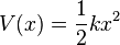
The potential energy stored in a simple harmonic oscillator at position x is

Damped harmonic oscillator


In real oscillators, friction, or damping, slows the motion of the system. Due to frictional force, the velocity decreases in proportion to the acting frictional force. While simple harmonic motion oscillates with only the restoring force acting on the system, damped harmonic motion experiences friction. In many vibrating systems the frictional force Ff can be modeled as being proportional to the velocity v of the object: Ff = −cv, where c is called the viscous damping coefficient.
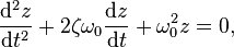
Balance of forces (Newton's second law) for damped harmonic oscillators is then

 ), this can be rewritten into the form
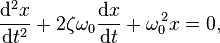
 is called the 'undamped angular frequency of the oscillator' and
 is called the 'undamped
  is called the 'damping ratio'.
 is called the 'damping ratio'.
The value of the damping ratio ζ critically determines the behavior of the system. A damped harmonic oscillator can be:
- Overdamped (ζ > 1): The system returns (exponentially decays) to steady state without oscillating. Larger values of the damping ratio ζ return to equilibrium slower.
- Critically damped (ζ = 1): The system returns to steady state as quickly as possible without oscillating (although overshoot can occur). This is often desired for the damping of systems such as doors.
- Underdamped (ζ < 1): The system oscillates (with a slightly different frequency than the undamped case) with the amplitude gradually decreasing to zero. The angular frequency of the underdamped harmonic oscillator is given by


Driven harmonic oscillators
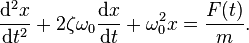
Driven harmonic oscillators are damped oscillators further affected by an externally applied force F(t).Newton's second law takes the form


Step input
In the case ζ < 1 and a unit step input with x(0) = 0:


In electrical engineering, a multiple of τ is called the settling time, i.e. the time necessary to ensure the signal is within a fixed departure from final value, typically within 10%. The term overshoot refers to the extent the maximum response exceeds final value, and undershoot refers to the extent the response falls below final value for times following the maximum response.
Sinusoidal driving force

Steady state variation of amplitude with relative frequency  and damping
  of a driven simple harmonic oscillator.
 and damping
  of a driven simple harmonic oscillator.
In the case of a sinusoidal driving force:

 is the driving amplitude and
  is the driving frequency for a sinusoidal driving mechanism. This type of system appears in AC driven RLC circuits (resistor-inductor-capacitor) and driven spring systems having internal mechanical resistance or external air resistance.
The general solution is a sum of a transient solution that depends on initial conditions, and a steady state that is independent of initial conditions and depends only on the driving amplitude
, driving frequency, , undamped angular frequency  , and the damping ratio
  .
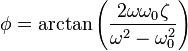
.The steady-state solution is proportional to the driving force with an induced phase change of
 :
:

For a particular driving frequency called the resonance, or resonant frequency
 , the amplitude (for a given ) is maximum. This resonance effect only occurs when
  , i.e. for significantly underdamped systems. For strongly underdamped systems the value of the amplitude can become quite large near the resonance frequency.
The transient solutions are the same as the unforced (
 ) damped harmonic oscillator and represent the systems response to other events that occurred previously. The transient solutions typically die out rapidly enough that they can be ignored.
Parametric oscillators
A parametric oscillator is a driven harmonic oscillator in which the drive energy is provided by varying the parameters of the oscillator, such as the damping or restoring force. A familiar example of parametric oscillation is "pumping" on a playground swing.[1][2][3] A person on a moving swing can increase the amplitude of the swing's oscillations without any external drive force (pushes) being applied, by changing the moment of inertia of the swing by rocking back and forth ("pumping") or alternately standing and squatting, in rhythm with the swing's oscillations.
The varying of the parameters drives the system. Examples of parameters that may be varied are its resonance frequency  and damping
  .
.
Parametric oscillators are used in many applications. The classical varactor parametric oscillator oscillates when the diode's capacitance is varied periodically. The circuit that varies the diode's capacitance is called the "pump" or "driver". In microwave electronics, waveguide/YAG based parametric oscillators operate in the same fashion. The designer varies a parameter periodically to induce oscillations.
Parametric oscillators have been developed as low-noise amplifiers, especially in the radio and microwave frequency range. Thermal noise is minimal, since a reactance (not a resistance) is varied. Another common use is frequency conversion, e.g., conversion from audio to radio frequencies. For example, the Optical parametric oscillator converts an input laser wave into two output waves of lower frequency ( ).
).
Parametric resonance occurs in a mechanical system when a system is parametrically excited and oscillates at one of its resonant frequencies. Parametric excitation differs from forcing, since the action appears as a time varying modification on a system parameter. This effect is different from regular resonance because it exhibits the instability phenomenon.
If the forcing function is f(t) = cos(ωt) = cos(ωtcτ) = cos(ωτ), where ω = ωtc, the equation becomes
![q_t (\tau) = \begin{cases} \mathrm{e}^{-\zeta\tau} \left( c_1 \mathrm{e}^{\tau \sqrt{\zeta^2 - 1}} + c_2 \mathrm{e}^{- \tau \sqrt{\zeta^2 - 1}} \right) & \zeta > 1 \text{ (overdamping)} \\ \mathrm{e}^{-\zeta\tau} (c_1+c_2 \tau) = \mathrm{e}^{-\tau}(c_1+c_2 \tau) & \zeta = 1 \text{ (critical damping)} \\ \mathrm{e}^{-\zeta \tau} \left[ c_1 \cos \left(\sqrt{1-\zeta^2} \tau\right) +c_2 \sin\left(\sqrt{1-\zeta^2} \tau\right) \right] & \zeta < 1 \text{(underdamping)} \end{cases}](//upload.wikimedia.org/math/2/8/8/2885f1873be326d16d8f9daac72ae585.png)
The transient solution is independent of the forcing function.
Squaring both equations and adding them together gives
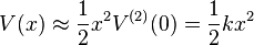
A conservative force is one that has a potential energy function. The potential energy function of a harmonic oscillator is:
 , one can do a Taylor expansion in terms of
  around an energy minimum (
 ) to model the behavior of small perturbations from equilibrium.
 is a minimum, the first derivative evaluated at
  must be zero, so the linear term drops out:
with a non-vanishing second derivative, one can use the solution to the simple harmonic oscillator to provide an approximate solution for small perturbations around the equilibrium point.
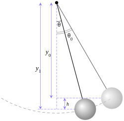
Assuming no damping and small amplitudes, the differential equation governing a simple pendulum is
 is the largest angle attained by the pendulum. The period, the time for one complete oscillation, is given by
  divided by whatever is multiplying the time in the argument of the cosine (
 here).
When a spring is stretched or compressed by a mass, the spring develops a restoring force. Hooke's law gives the relationship of the force exerted by the spring when the spring is compressed or stretched a certain length:
By using either force balance or an energy method, it can be readily shown that the motion of this system is given by the following differential equation:
If the initial displacement is A, and there is no initial velocity, the solution of this equation is given by:
 is the mass on the end of the spring. If the spring itself has mass, its effective mass must be included in .

When the spring is stretched or compressed, kinetic energy of the mass gets converted into potential energy of the spring. By conservation of energy, assuming the datum is defined at the equilibrium position, when the spring reaches its maximum potential energy, the kinetic energy of the mass is zero. When the spring is released, it tries to return to equilibrium, and all its potential energy converts to kinetic energy of the mass.
 and damping
  .
.Parametric oscillators are used in many applications. The classical varactor parametric oscillator oscillates when the diode's capacitance is varied periodically. The circuit that varies the diode's capacitance is called the "pump" or "driver". In microwave electronics, waveguide/YAG based parametric oscillators operate in the same fashion. The designer varies a parameter periodically to induce oscillations.
Parametric oscillators have been developed as low-noise amplifiers, especially in the radio and microwave frequency range. Thermal noise is minimal, since a reactance (not a resistance) is varied. Another common use is frequency conversion, e.g., conversion from audio to radio frequencies. For example, the Optical parametric oscillator converts an input laser wave into two output waves of lower frequency (
 ).
).Parametric resonance occurs in a mechanical system when a system is parametrically excited and oscillates at one of its resonant frequencies. Parametric excitation differs from forcing, since the action appears as a time varying modification on a system parameter. This effect is different from regular resonance because it exhibits the instability phenomenon.
Universal oscillator equation
The equation
If the forcing function is f(t) = cos(ωt) = cos(ωtcτ) = cos(ωτ), where ω = ωtc, the equation becomes

Transient solution
The solution based on solving the ordinary differential equation is for arbitrary constants c1 and c2![q_t (\tau) = \begin{cases} \mathrm{e}^{-\zeta\tau} \left( c_1 \mathrm{e}^{\tau \sqrt{\zeta^2 - 1}} + c_2 \mathrm{e}^{- \tau \sqrt{\zeta^2 - 1}} \right) & \zeta > 1 \text{ (overdamping)} \\ \mathrm{e}^{-\zeta\tau} (c_1+c_2 \tau) = \mathrm{e}^{-\tau}(c_1+c_2 \tau) & \zeta = 1 \text{ (critical damping)} \\ \mathrm{e}^{-\zeta \tau} \left[ c_1 \cos \left(\sqrt{1-\zeta^2} \tau\right) +c_2 \sin\left(\sqrt{1-\zeta^2} \tau\right) \right] & \zeta < 1 \text{(underdamping)} \end{cases}](http://upload.wikimedia.org/math/2/8/8/2885f1873be326d16d8f9daac72ae585.png)
The transient solution is independent of the forcing function.
Steady-state solution
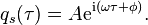
Apply the "complex variables method" by solving the auxiliary equation below and then finding the real part of its solution:


Amplitude part

Squaring both equations and adding them together gives
![\left . \begin{array}{rcl} A^2 (1-\omega^2)^2 & = & \cos^2\phi \\[6pt] (2 \zeta \omega A)^2 & = & \sin^2\phi \end{array} \right \} \Rightarrow A^2[(1-\omega^2)^2 + (2 \zeta \omega)^2] = 1.](http://upload.wikimedia.org/math/6/2/2/622f099529705ddd1b3307db1c99f83f.png)

Phase part
To solve for φ, divide both equations to get
Full solution
Combining the amplitude and phase portions results in the steady-state solution
Equivalent systems
Harmonic oscillators occurring in a number of areas of engineering are equivalent in the sense that their mathematical models are identical (see universal oscillator equation above). Below is a table showing analogous quantities in four harmonic oscillator systems in mechanics and electronics. If analogous parameters on the same line in the table are given numerically equal values, the behavior of the oscillators—their output waveform, resonant frequency, damping factor, etc.—are the same.| Translational Mechanical | Torsional Mechanical | Series RLC Circuit | Parallel RLC Circuit |
|---|---|---|---|
Position  |
Angle  |
Charge  |
Flux linkage  |
Velocity  |
Angular velocity  |
Current  |
Voltage  |
Mass  |
Moment of inertia  |
Inductance  |
Capacitance  |
Spring constant  |
Torsion constant  |
Elastance  |
Susceptance  |
Damping  |
Rotational friction  |
Resistance  |
Conductance  |
Drive force  |
Drive torque  |
Voltage  |
Current  |
Undamped resonant frequency  : : |
|||
 |
 |
 |
|
| Differential equation: | |||
 |
 |
 |
 |
Application to a conservative force
The problem of the simple harmonic oscillator occurs frequently in physics, because a mass at equilibrium under the influence of any conservative force, in the limit of small motions, behaves as a simple harmonic oscillator.A conservative force is one that has a potential energy function. The potential energy function of a harmonic oscillator is:
 , one can do a Taylor expansion in terms of
  around an energy minimum (
 ) to model the behavior of small perturbations from equilibrium.
 is a minimum, the first derivative evaluated at
  must be zero, so the linear term drops out:
 with a non-vanishing second derivative, one can use the solution to the simple harmonic oscillator to provide an approximate solution for small perturbations around the equilibrium point.
Examples
Simple pendulum

A simple pendulum exhibits simple harmonic motion under the conditions of no damping and small amplitude.
Assuming no damping and small amplitudes, the differential equation governing a simple pendulum is


 is the largest angle attained by the pendulum. The period, the time for one complete oscillation, is given by
  divided by whatever is multiplying the time in the argument of the cosine (
 here).
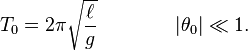
Pendulum swinging over turntable
Simple harmonic motion can in some cases be considered to be the one-dimensional projection of two-dimensional circular motion. Consider a long pendulum swinging over the turntable of a record player. On the edge of the turntable there is an object. If the object is viewed from the same level as the turntable, a projection of the motion of the object seems to be moving backwards and forwards on a straight line orthogonal to the view direction, sinusoidally like the pendulum.Spring/mass system

When a spring is stretched or compressed by a mass, the spring develops a restoring force. Hooke's law gives the relationship of the force exerted by the spring when the spring is compressed or stretched a certain length:

By using either force balance or an energy method, it can be readily shown that the motion of this system is given by the following differential equation:

If the initial displacement is A, and there is no initial velocity, the solution of this equation is given by:
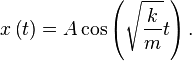
 is the mass on the end of the spring. If the spring itself has mass, its effective mass must be included in .
Energy variation in the spring–damping system
In terms of energy, all systems have two types of energy, potential energy and kinetic energy. When a spring is stretched or compressed, it stores elastic potential energy, which then is transferred into kinetic energy. The potential energy within a spring is determined by the equation
When the spring is stretched or compressed, kinetic energy of the mass gets converted into potential energy of the spring. By conservation of energy, assuming the datum is defined at the equilibrium position, when the spring reaches its maximum potential energy, the kinetic energy of the mass is zero. When the spring is released, it tries to return to equilibrium, and all its potential energy converts to kinetic energy of the mass.


