Stable nuclide

From Wikipedia, the free encyclopedia

https://en.wikipedia.org/wiki/Stable_nuclide 

 

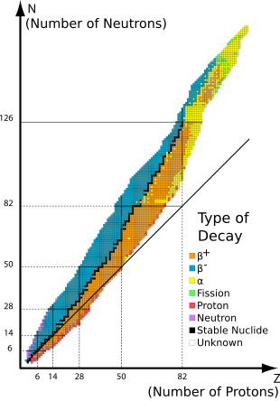
Graph of nuclides (isotopes) by type of decay. Orange and blue nuclides are unstable, with the black squares between these regions representing stable nuclides. The continuous line passing below most of the nuclides comprises the positions on the graph of the (mostly hypothetical) nuclides for which proton number would the same as neutron number. The graph reflects the fact that elements with more than 20 protons either have more neutrons than protons or are unstable.

Stable nuclides are nuclides that are not radioactive and so (unlike radionuclides) do not spontaneously undergo radioactive decay. When such nuclides are referred to in relation to specific elements, they are usually termed stable isotopes.

The 80 elements with one or more stable isotopes comprise a total of 252 nuclides that have not been known to decay using current equipment (see list at the end of this article). Of these elements, 26 have only one stable isotope; they are thus termed monoisotopic. The rest have more than one stable isotope. Tin has ten stable isotopes, the largest number of stable isotopes known for an element.

Definition of stability, and naturally occurring nuclides

Most naturally occurring nuclides are stable (about 252; see list at the end of this article), and about 34 more (total of 286) are known to be radioactive with sufficiently long half-lives (also known) to occur primordially. If the half-life of a nuclide is comparable to, or greater than, the Earth's age (4.5 billion years), a significant amount will have survived since the formation of the Solar System, and then is said to be primordial. It will then contribute in that way to the natural isotopic composition of a chemical element. Primordially present radioisotopes are easily detected with half-lives as short as 700 million years (e.g., ²³⁵U). This is the present limit of detection, as shorter-lived nuclides have not yet been detected undisputedly in nature.

Many naturally occurring radioisotopes (another 53 or so, for a total of about 339) exhibit still shorter half-lives than 700 million years, but they are made freshly, as daughter products of decay processes of primordial nuclides (for example, radium from uranium) or from ongoing energetic reactions, such as cosmogenic nuclides produced by present bombardment of Earth by cosmic rays (for example, ¹⁴C made from nitrogen).

Some isotopes that are classed as stable (i.e. no radioactivity has been observed for them) are predicted to have extremely long half-lives (sometimes as high as 10¹⁸ years or more). If the predicted half-life falls into an experimentally accessible range, such isotopes have a chance to move from the list of stable nuclides to the radioactive category, once their activity is observed. For example, ²⁰⁹Bi and ¹⁸⁰W were formerly classed as stable, but were found to be alpha-active in 2003. However, such nuclides do not change their status as primordial when they are found to be radioactive.

Most stable isotopes on Earth are believed to have been formed in processes of nucleosynthesis, either in the Big Bang, or in generations of stars that preceded the formation of the solar system. However, some stable isotopes also show abundance variations in the earth as a result of decay from long-lived radioactive nuclides. These decay-products are termed radiogenic isotopes, in order to distinguish them from the much larger group of 'non-radiogenic' isotopes.

Isotopes per element

Of the known chemical elements, 80 elements have at least one stable nuclide. These comprise the first 82 elements from hydrogen to lead, with the two exceptions, technetium (element 43) and promethium (element 61), that do not have any stable nuclides. As of December 2016, there were a total of 252 known "stable" nuclides. In this definition, "stable" means a nuclide that has never been observed to decay against the natural background. Thus, these elements have half lives too long to be measured by any means, direct or indirect.

Stable isotopes:

• 1 element (tin) has 10 stable isotopes
• 5 elements have 7 stable isotopes apiece
• 7 elements have 6 stable isotopes apiece
• 11 elements have 5 stable isotopes apiece
• 9 elements have 4 stable isotopes apiece
• 5 elements have 3 stable isotopes apiece
• 16 elements have 2 stable isotopes apiece
• 26 elements have 1 single stable isotope.

These last 26 are thus called monoisotopic elements. The mean number of stable isotopes for elements which have at least one stable isotope is 252/80 = 3.15.

Physical magic numbers and odd and even proton and neutron count

Stability of isotopes is affected by the ratio of protons to neutrons, and also by presence of certain magic numbers of neutrons or protons which represent closed and filled quantum shells. These quantum shells correspond to a set of energy levels within the shell model of the nucleus; filled shells, such as the filled shell of 50 protons for tin, confers unusual stability on the nuclide. As in the case of tin, a magic number for Z, the atomic number, tends to increase the number of stable isotopes for the element.

Just as in the case of electrons, which have the lowest energy state when they occur in pairs in a given orbital, nucleons (both protons and neutrons) exhibit a lower energy state when their number is even, rather than odd. This stability tends to prevent beta decay (in two steps) of many even–even nuclides into another even–even nuclide of the same mass number but lower energy (and of course with two more protons and two fewer neutrons), because decay proceeding one step at a time would have to pass through an odd–odd nuclide of higher energy. Such nuclei thus instead undergo double beta decay (or are theorized to do so) with half-lives several orders of magnitude larger than the age of the universe. This makes for a larger number of stable even-even nuclides, which account for 151 of the 252 total. Stable even–even nuclides number as many as three isobars for some mass numbers, and up to seven isotopes for some atomic numbers.

Conversely, of the 252 known stable nuclides, only five have both an odd number of protons and odd number of neutrons: hydrogen-2 (deuterium), lithium-6, boron-10, nitrogen-14, and tantalum-180m. Also, only four naturally occurring, radioactive odd–odd nuclides have a half-life over a billion years: potassium-40, vanadium-50, lanthanum-138, and lutetium-176. Odd–odd primordial nuclides are rare because most odd–odd nuclei are unstable with respect to beta decay, because the decay products are even–even, and are therefore more strongly bound, due to nuclear pairing effects.

Yet another effect of the instability of an odd number of either type of nucleons is that odd-numbered elements tend to have fewer stable isotopes. Of the 26 monoisotopic elements (those with only a single stable isotope), all but one have an odd atomic number, and all but one has an even number of neutrons—the single exception to both rules being beryllium.

The end of the stable elements in the periodic table occurs after lead, largely due to the fact that nuclei with 128 neutrons are extraordinarily unstable and almost immediately shed alpha particles. This also contributes to the very short half-lives of astatine, radon, and francium relative to heavier elements. This may also be seen to a much lesser extent with 84 neutrons, which exhibits as a certain number of isotopes in the lanthanide series which exhibit alpha decay.

Nuclear isomers, including a "stable" one

The count of 252 known stable nuclides includes tantalum-180m, since even though its decay and instability is automatically implied by its notation of "metastable", this has still not yet been observed. All "stable" isotopes (stable by observation, not theory) are the ground states of nuclei, with the exception of tantalum-180m, which is a nuclear isomer or excited state. The ground state of this particular nucleus, tantalum-180, is radioactive with a comparatively short half-life of 8 hours; in contrast, the decay of the excited nuclear isomer is extremely strongly forbidden by spin-parity selection rules. It has been reported experimentally by direct observation that the half-life of ^180mTa to gamma decay must be more than 10¹⁵ years. Other possible modes of ^180mTa decay (beta decay, electron capture and alpha decay) have also never been observed.

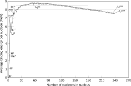
Binding energy per nucleon of common isotopes.

Still-unobserved decay

It is expected that some continual improvement of experimental sensitivity will allow discovery of very mild radioactivity (instability) of some isotopes that are considered to be stable today. For an example of a recent discovery, it was not until 2003 that bismuth-209 (the only primordial isotope of bismuth) was shown to be very mildly radioactive, confirming theoretical predictions from nuclear physics that bismuth-209 would decay very slowly by alpha emission.

Isotopes that are theoretically believed to be unstable but have not been observed to decay are termed as observationally stable.

Summary table for numbers of each class of nuclides

This is a summary table from List of nuclides. Note that numbers are not exact and may change slightly in the future, as nuclides are observed to be radioactive, or new half-lives are determined to some precision.

Type of nuclide by stability class	Number of nuclides in class	Running total of nuclides in all classes to this point	Notes
Theoretically stable to all but proton decay	90	90	Includes first 40 elements. If protons decay, then there are no stable nuclides.
Theoretically stable to alpha decay, beta decay, isomeric transition, and double beta decay but not spontaneous fission, which is possible for "stable" nuclides ≥ niobium-93	56	146	(Note that spontaneous fission has never been observed for nuclides with mass number < 230).
Energetically unstable to one or more known decay modes, but no decay yet seen. Considered stable until radioactivity confirmed.	106	252	Total is the observationally stable nuclides.
Radioactive primordial nuclides.	34	286	Includes Bi, Th, U.
Radioactive nonprimordial, but naturally occurring on Earth.	~61 significant	~347 significant	Cosmogenic nuclides from cosmic rays; daughters of radioactive primordials such as francium, etc.

List of stable nuclides

1. Hydrogen-1
2. Hydrogen-2
3. Helium-3
4. Helium-4

   no mass number 5

5. Lithium-6
6. Lithium-7
   no mass number 8
7. Beryllium-9
8. Boron-10
9. Boron-11
10. Carbon-12
11. Carbon-13
12. Nitrogen-14
13. Nitrogen-15
14. Oxygen-16
15. Oxygen-17
16. Oxygen-18
17. Fluorine-19
18. Neon-20
19. Neon-21
20. Neon-22
21. Sodium-23
22. Magnesium-24
23. Magnesium-25
24. Magnesium-26
25. Aluminium-27
26. Silicon-28
27. Silicon-29
28. Silicon-30
29. Phosphorus-31
30. Sulfur-32
31. Sulfur-33
32. Sulfur-34
33. Sulfur-36
34. Chlorine-35
35. Chlorine-37
36. Argon-36 (2E)
37. Argon-38
38. Argon-40
39. Potassium-39
40. Potassium-41
41. Calcium-40 (2E)*
42. Calcium-42
43. Calcium-43
44. Calcium-44
45. Calcium-46 (2B)*
46. Scandium-45
47. Titanium-46
48. Titanium-47
49. Titanium-48
50. Titanium-49
51. Titanium-50
52. Vanadium-51
53. Chromium-50 (2E)*
54. Chromium-52
55. Chromium-53
56. Chromium-54
57. Manganese-55
58. Iron-54 (2E)*
59. Iron-56
60. Iron-57
61. Iron-58
62. Cobalt-59
63. Nickel-58 (2E)*
64. Nickel-60
65. Nickel-61
66. Nickel-62
67. Nickel-64
68. Copper-63
69. Copper-65
70. Zinc-64 (2E)*
71. Zinc-66
72. Zinc-67
73. Zinc-68
74. Zinc-70 (2B)*
75. Gallium-69
76. Gallium-71
77. Germanium-70
78. Germanium-72
79. Germanium-73
80. Germanium-74
81. Arsenic-75
82. Selenium-74 (2E)
83. Selenium-76
84. Selenium-77
85. Selenium-78
86. Selenium-80 (2B)
87. Bromine-79
88. Bromine-81
89. Krypton-80
90. Krypton-82
91. Krypton-83
92. Krypton-84
93. Krypton-86 (2B)
94. Rubidium-85
95. Strontium-84 (2E)
96. Strontium-86
97. Strontium-87
98. Strontium-88
99. Yttrium-89
100. Zirconium-90
101. Zirconium-91
102. Zirconium-92
103. Zirconium-94 (2B)*
104. Niobium-93
105. Molybdenum-92 (2E)*
106. Molybdenum-94
107. Molybdenum-95
108. Molybdenum-96
109. Molybdenum-97
110. Molybdenum-98 (2B)*
     Technetium - No stable isotopes
111. Ruthenium-96 (2E)*
112. Ruthenium-98
113. Ruthenium-99
114. Ruthenium-100
115. Ruthenium-101
116. Ruthenium-102
117. Ruthenium-104 (2B)
118. Rhodium-103
119. Palladium-102 (2E)
120. Palladium-104
121. Palladium-105
122. Palladium-106
123. Palladium-108
124. Palladium-110 (2B)*
125. Silver-107
126. Silver-109
127. Cadmium-106 (2E)*
128. Cadmium-108 (2E)*
129. Cadmium-110
130. Cadmium-111
131. Cadmium-112
132. Cadmium-114 (2B)*
133. Indium-113
134. Tin-112 (2E)
135. Tin-114
136. Tin-115
137. Tin-116
138. Tin-117
139. Tin-118
140. Tin-119
141. Tin-120
142. Tin-122 (2B)
143. Tin-124 (2B)*
144. Antimony-121
145. Antimony-123
146. Tellurium-120 (2E)*
147. Tellurium-122
148. Tellurium-123 (E)*
149. Tellurium-124
150. Tellurium-125
151. Tellurium-126
152. Iodine-127
153. Xenon-126 (2E)
154. Xenon-128
155. Xenon-129
156. Xenon-130
157. Xenon-131
158. Xenon-132
159. Xenon-134 (2B)*
160. Caesium-133
161. Barium-132 (2E)*
162. Barium-134
163. Barium-135
164. Barium-136
165. Barium-137
166. Barium-138
167. Lanthanum-139
168. Cerium-136 (2E)*
169. Cerium-138 (2E)*
170. Cerium-140
171. Cerium-142 (A, 2B)*
172. Praseodymium-141
173. Neodymium-142
174. Neodymium-143
175. Neodymium-145 (A)*
176. Neodymium-146 (2B)
     no mass number 147
177. Neodymium-148 (A, 2B)*
     Promethium - No stable isotopes
178. Samarium-144 (2E)
179. Samarium-149 (A)*
180. Samarium-150
     no mass number 151
181. Samarium-152
182. Samarium-154 (2B)*
183. Europium-153
184. Gadolinium-154
185. Gadolinium-155
186. Gadolinium-156
187. Gadolinium-157
188. Gadolinium-158
189. Gadolinium-160 (2B)*
190. Terbium-159
191. Dysprosium-156 (A, 2E)*
192. Dysprosium-158
193. Dysprosium-160
194. Dysprosium-161
195. Dysprosium-162
196. Dysprosium-163
197. Dysprosium-164
198. Holmium-165
199. Erbium-162 (A, 2E)*
200. Erbium-164
201. Erbium-166
202. Erbium-167
203. Erbium-168
204. Erbium-170 (A, 2B)*
205. Thulium-169
206. Ytterbium-168 (A, 2E)*
207. Ytterbium-170
208. Ytterbium-171
209. Ytterbium-172
210. Ytterbium-173
211. Ytterbium-174
212. Ytterbium-176 (A, 2B)*
213. Lutetium-175
214. Hafnium-176
215. Hafnium-177
216. Hafnium-178
217. Hafnium-179
218. Hafnium-180
219. Tantalum-180m (A, B, E, IT)* ^
220. Tantalum-181
221. Tungsten-182 (A)*
222. Tungsten-183 (A)*
223. Tungsten-184 (A)*
224. Tungsten-186 (A, 2B)*
225. Rhenium-185
226. Osmium-184 (A, 2E)*
227. Osmium-187
228. Osmium-188
229. Osmium-189
230. Osmium-190
231. Osmium-192 (A, 2B)*
232. Iridium-191
233. Iridium-193
234. Platinum-192 (A)*
235. Platinum-194
236. Platinum-195
237. Platinum-196
238. Platinum-198 (A, 2B)*
239. Gold-197
240. Mercury-196 (A, 2E)*
241. Mercury-198
242. Mercury-199
243. Mercury-200
244. Mercury-201
245. Mercury-202
246. Mercury-204 (2B)
247. Thallium-203
248. Thallium-205
249. Lead-204 (A)*
250. Lead-206 (A)
251. Lead-207 (A)
252. Lead-208 (A)*
     Bismuth ^^ and above – No stable isotopes
     no mass number 209 and above

Abbreviations for predicted unobserved decay:

A for alpha decay, B for beta decay, 2B for double beta decay, E for electron capture, 2E for double electron capture, IT for isomeric transition, SF for spontaneous fission, * for the nuclides whose half-lives have lower bound.

^ Tantalum-180m is a "metastable isotope" meaning that it is an excited nuclear isomer of tantalum-180. See isotopes of tantalum. However, the half-life of this nuclear isomer is so long that it has never been observed to decay, and it thus occurs as an "observationally nonradioactive" primordial nuclide, as a minor isotope of tantalum. This is the only case of a nuclear isomer which has a half-life so long that it has never been observed to decay. It is thus included in this list.

^^ Bismuth-209 had long been believed to be stable, due to its unusually long half-life of 2.01×10¹⁹ years, which is more than a billion (1000 million) times the age of the universe.

Computer simulation

From Wikipedia, the free encyclopedia

https://en.wikipedia.org/wiki/Computer_simulation 

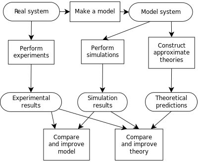
Process of building a computer model, and the interplay between experiment, simulation, and theory.

Computer simulation is the process of mathematical modelling, performed on a computer, which is designed to predict the behaviour of or the outcome of a real-world or physical system. Since they allow to check the reliability of chosen mathematical models, computer simulations have become a useful tool for the mathematical modeling of many natural systems in physics (computational physics), astrophysics, climatology, chemistry, biology and manufacturing, as well as human systems in economics, psychology, social science, health care and engineering. Simulation of a system is represented as the running of the system's model. It can be used to explore and gain new insights into new technology and to estimate the performance of systems too complex for analytical solutions.

Computer simulations are realized by running computer programs that can be either small, running almost instantly on small devices, or large-scale programs that run for hours or days on network-based groups of computers. The scale of events being simulated by computer simulations has far exceeded anything possible (or perhaps even imaginable) using traditional paper-and-pencil mathematical modeling. In 1997, a desert-battle simulation of one force invading another involved the modeling of 66,239 tanks, trucks and other vehicles on simulated terrain around Kuwait, using multiple supercomputers in the DoD High Performance Computer Modernization Program. Other examples include a 1-billion-atom model of material deformation; a 2.64-million-atom model of the complex protein-producing organelle of all living organisms, the ribosome, in 2005; a complete simulation of the life cycle of Mycoplasma genitalium in 2012; and the Blue Brain project at EPFL (Switzerland), begun in May 2005 to create the first computer simulation of the entire human brain, right down to the molecular level.

Because of the computational cost of simulation, computer experiments are used to perform inference such as uncertainty quantification.

Simulation versus model

A computer model is the algorithms and equations used to capture the behavior of the system being modeled. By contrast, computer simulation is the actual running of the program that contains these equations or algorithms. Simulation, therefore, is the process of running a model. Thus one would not "build a simulation"; instead, one would "build a model", and then either "run the model" or equivalently "run a simulation".

History

Computer simulation developed hand-in-hand with the rapid growth of the computer, following its first large-scale deployment during the Manhattan Project in World War II to model the process of nuclear detonation. It was a simulation of 12 hard spheres using a Monte Carlo algorithm. Computer simulation is often used as an adjunct to, or substitute for, modeling systems for which simple closed form analytic solutions are not possible. There are many types of computer simulations; their common feature is the attempt to generate a sample of representative scenarios for a model in which a complete enumeration of all possible states of the model would be prohibitive or impossible.

Data preparation

The external data requirements of simulations and models vary widely. For some, the input might be just a few numbers (for example, simulation of a waveform of AC electricity on a wire), while others might require terabytes of information (such as weather and climate models).

Input sources also vary widely:

• Sensors and other physical devices connected to the model;
• Control surfaces used to direct the progress of the simulation in some way;
• Current or historical data entered by hand;
• Values extracted as a by-product from other processes;
• Values output for the purpose by other simulations, models, or processes.

Lastly, the time at which data is available varies:

• "invariant" data is often built into the model code, either because the value is truly invariant (e.g., the value of π) or because the designers consider the value to be invariant for all cases of interest;
• data can be entered into the simulation when it starts up, for example by reading one or more files, or by reading data from a preprocessor;
• data can be provided during the simulation run, for example by a sensor network.

Because of this variety, and because diverse simulation systems have many common elements, there are a large number of specialized simulation languages. The best-known may be Simula (sometimes called Simula-67, after the year 1967 when it was proposed). There are now many others.

Systems that accept data from external sources must be very careful in knowing what they are receiving. While it is easy for computers to read in values from text or binary files, what is much harder is knowing what the accuracy (compared to measurement resolution and precision) of the values are. Often they are expressed as "error bars", a minimum and maximum deviation from the value range within which the true value (is expected to) lie. Because digital computer mathematics is not perfect, rounding and truncation errors multiply this error, so it is useful to perform an "error analysis" to confirm that values output by the simulation will still be usefully accurate.

Types

Computer models can be classified according to several independent pairs of attributes, including:

• Stochastic or deterministic (and as a special case of deterministic, chaotic) – see external links below for examples of stochastic vs. deterministic simulations
• Steady-state or dynamic
• Continuous or discrete (and as an important special case of discrete, discrete event or DE models)
• Dynamic system simulation, e.g. electric systems, hydraulic systems or multi-body mechanical systems (described primarily by DAE:s) or dynamics simulation of field problems, e.g. CFD of FEM simulations (described by PDE:s).
• Local or distributed.

Another way of categorizing models is to look at the underlying data structures. For time-stepped simulations, there are two main classes:

• Simulations which store their data in regular grids and require only next-neighbor access are called stencil codes. Many CFD applications belong to this category.
• If the underlying graph is not a regular grid, the model may belong to the meshfree method class.

Equations define the relationships between elements of the modeled system and attempt to find a state in which the system is in equilibrium. Such models are often used in simulating physical systems, as a simpler modeling case before dynamic simulation is attempted.

• Dynamic simulations model changes in a system in response to (usually changing) input signals.
• Stochastic models use random number generators to model chance or random events;
• A discrete event simulation (DES) manages events in time. Most computer, logic-test and fault-tree simulations are of this type. In this type of simulation, the simulator maintains a queue of events sorted by the simulated time they should occur. The simulator reads the queue and triggers new events as each event is processed. It is not important to execute the simulation in real time. It is often more important to be able to access the data produced by the simulation and to discover logic defects in the design or the sequence of events.
• A continuous dynamic simulation performs numerical solution of differential-algebraic equations or differential equations (either partial or ordinary). Periodically, the simulation program solves all the equations and uses the numbers to change the state and output of the simulation. Applications include flight simulators, construction and management simulation games, chemical process modeling, and simulations of electrical circuits. Originally, these kinds of simulations were actually implemented on analog computers, where the differential equations could be represented directly by various electrical components such as op-amps. By the late 1980s, however, most "analog" simulations were run on conventional digital computers that emulate the behavior of an analog computer.
• A special type of discrete simulation that does not rely on a model with an underlying equation, but can nonetheless be represented formally, is agent-based simulation. In agent-based simulation, the individual entities (such as molecules, cells, trees or consumers) in the model are represented directly (rather than by their density or concentration) and possess an internal state and set of behaviors or rules that determine how the agent's state is updated from one time-step to the next.
• Distributed models run on a network of interconnected computers, possibly through the Internet. Simulations dispersed across multiple host computers like this are often referred to as "distributed simulations". There are several standards for distributed simulation, including Aggregate Level Simulation Protocol (ALSP), Distributed Interactive Simulation (DIS), the High Level Architecture (simulation) (HLA) and the Test and Training Enabling Architecture (TENA).

Visualization

Formerly, the output data from a computer simulation was sometimes presented in a table or a matrix showing how data were affected by numerous changes in the simulation parameters. The use of the matrix format was related to traditional use of the matrix concept in mathematical models. However, psychologists and others noted that humans could quickly perceive trends by looking at graphs or even moving-images or motion-pictures generated from the data, as displayed by computer-generated-imagery (CGI) animation. Although observers could not necessarily read out numbers or quote math formulas, from observing a moving weather chart they might be able to predict events (and "see that rain was headed their way") much faster than by scanning tables of rain-cloud coordinates. Such intense graphical displays, which transcended the world of numbers and formulae, sometimes also led to output that lacked a coordinate grid or omitted timestamps, as if straying too far from numeric data displays. Today, weather forecasting models tend to balance the view of moving rain/snow clouds against a map that uses numeric coordinates and numeric timestamps of events.

Similarly, CGI computer simulations of CAT scans can simulate how a tumor might shrink or change during an extended period of medical treatment, presenting the passage of time as a spinning view of the visible human head, as the tumor changes.

Other applications of CGI computer simulations are being developed to graphically display large amounts of data, in motion, as changes occur during a simulation run.

Computer simulation in science

Computer simulation of the process of osmosis

Generic examples of types of computer simulations in science, which are derived from an underlying mathematical description:

• a numerical simulation of differential equations that cannot be solved analytically, theories that involve continuous systems such as phenomena in physical cosmology, fluid dynamics (e.g., climate models, roadway noise models, roadway air dispersion models), continuum mechanics and chemical kinetics fall into this category.
• a stochastic simulation, typically used for discrete systems where events occur probabilistically and which cannot be described directly with differential equations (this is a discrete simulation in the above sense). Phenomena in this category include genetic drift, biochemical or gene regulatory networks with small numbers of molecules.
• multiparticle simulation of the response of nanomaterials at multiple scales to an applied force for the purpose of modeling their thermoelastic and thermodynamic properties. Techniques used for such simulations are Molecular dynamics, Molecular mechanics, Monte Carlo method, and Multiscale Green's function.

Specific examples of computer simulations follow:

• statistical simulations based upon an agglomeration of a large number of input profiles, such as the forecasting of equilibrium temperature of receiving waters, allowing the gamut of meteorological data to be input for a specific locale. This technique was developed for thermal pollution forecasting.
• agent based simulation has been used effectively in ecology, where it is often called "individual based modeling" and is used in situations for which individual variability in the agents cannot be neglected, such as population dynamics of salmon and trout (most purely mathematical models assume all trout behave identically).
• time stepped dynamic model. In hydrology there are several such hydrology transport models such as the SWMM and DSSAM Models developed by the U.S. Environmental Protection Agency for river water quality forecasting.
• computer simulations have also been used to formally model theories of human cognition and performance, e.g., ACT-R.
• computer simulation using molecular modeling for drug discovery.
• computer simulation to model viral infection in mammalian cells.
• computer simulation for studying the selective sensitivity of bonds by mechanochemistry during grinding of organic molecules.
• Computational fluid dynamics simulations are used to simulate the behaviour of flowing air, water and other fluids. One-, two- and three-dimensional models are used. A one-dimensional model might simulate the effects of water hammer in a pipe. A two-dimensional model might be used to simulate the drag forces on the cross-section of an aeroplane wing. A three-dimensional simulation might estimate the heating and cooling requirements of a large building.
• An understanding of statistical thermodynamic molecular theory is fundamental to the appreciation of molecular solutions. Development of the Potential Distribution Theorem (PDT) allows this complex subject to be simplified to down-to-earth presentations of molecular theory.

Notable, and sometimes controversial, computer simulations used in science include: Donella Meadows' World3 used in the Limits to Growth, James Lovelock's Daisyworld and Thomas Ray's Tierra.

In social sciences, computer simulation is an integral component of the five angles of analysis fostered by the data percolation methodology, which also includes qualitative and quantitative methods, reviews of the literature (including scholarly), and interviews with experts, and which forms an extension of data triangulation. Of course, similar to any other scientific method, replication is an important part of computational modeling 

Simulation environments for physics and engineering

Graphical environments to design simulations have been developed. Special care was taken to handle events (situations in which the simulation equations are not valid and have to be changed). The open project Open Source Physics was started to develop reusable libraries for simulations in Java, together with Easy Java Simulations, a complete graphical environment that generates code based on these libraries.

Simulation environments for linguistics

Taiwanese Tone Group Parser is a simulator of Taiwanese tone sandhi acquisition. In practical, the method using linguistic theory to implement the Taiwanese tone group parser is a way to apply knowledge engineering technique to build the experiment environment of computer simulation for language acquisition. A work-in-process version of artificial tone group parser that includes a knowledge base and an executable program file for Microsoft Windows system (XP/Win7) can be download for evaluation.

Computer simulation in practical contexts

Computer simulations are used in a wide variety of practical contexts, such as:

• analysis of air pollutant dispersion using atmospheric dispersion modeling
• design of complex systems such as aircraft and also logistics systems.
• design of noise barriers to effect roadway noise mitigation
• modeling of application performance
• flight simulators to train pilots
• weather forecasting
• forecasting of risk
• simulation of electrical circuits
• Power system simulation
• simulation of other computers is emulation.
• forecasting of prices on financial markets (for example Adaptive Modeler)
• behavior of structures (such as buildings and industrial parts) under stress and other conditions
• design of industrial processes, such as chemical processing plants
• strategic management and organizational studies
• reservoir simulation for the petroleum engineering to model the subsurface reservoir
• process engineering simulation tools.
• robot simulators for the design of robots and robot control algorithms
• urban simulation models that simulate dynamic patterns of urban development and responses to urban land use and transportation policies. See a more detailed article on Urban Environment Simulation.
• traffic engineering to plan or redesign parts of the street network from single junctions over cities to a national highway network to transportation system planning, design and operations. See a more detailed article on Simulation in Transportation.
• modeling car crashes to test safety mechanisms in new vehicle models.
• crop-soil systems in agriculture, via dedicated software frameworks (e.g. BioMA, OMS3, APSIM)

The reliability and the trust people put in computer simulations depends on the validity of the simulation model, therefore verification and validation are of crucial importance in the development of computer simulations. Another important aspect of computer simulations is that of reproducibility of the results, meaning that a simulation model should not provide a different answer for each execution. Although this might seem obvious, this is a special point of attention in stochastic simulations, where random numbers should actually be semi-random numbers. An exception to reproducibility are human-in-the-loop simulations such as flight simulations and computer games. Here a human is part of the simulation and thus influences the outcome in a way that is hard, if not impossible, to reproduce exactly.

Vehicle manufacturers make use of computer simulation to test safety features in new designs. By building a copy of the car in a physics simulation environment, they can save the hundreds of thousands of dollars that would otherwise be required to build and test a unique prototype. Engineers can step through the simulation milliseconds at a time to determine the exact stresses being put upon each section of the prototype.

Computer graphics can be used to display the results of a computer simulation. Animations can be used to experience a simulation in real-time, e.g., in training simulations. In some cases animations may also be useful in faster than real-time or even slower than real-time modes. For example, faster than real-time animations can be useful in visualizing the buildup of queues in the simulation of humans evacuating a building. Furthermore, simulation results are often aggregated into static images using various ways of scientific visualization.

In debugging, simulating a program execution under test (rather than executing natively) can detect far more errors than the hardware itself can detect and, at the same time, log useful debugging information such as instruction trace, memory alterations and instruction counts. This technique can also detect buffer overflow and similar "hard to detect" errors as well as produce performance information and tuning data.

Pitfalls

Although sometimes ignored in computer simulations, it is very important to perform a sensitivity analysis to ensure that the accuracy of the results is properly understood. For example, the probabilistic risk analysis of factors determining the success of an oilfield exploration program involves combining samples from a variety of statistical distributions using the Monte Carlo method. If, for instance, one of the key parameters (e.g., the net ratio of oil-bearing strata) is known to only one significant figure, then the result of the simulation might not be more precise than one significant figure, although it might (misleadingly) be presented as having four significant figures.

Model calibration techniques

The following three steps should be used to produce accurate simulation models: calibration, verification, and validation. Computer simulations are good at portraying and comparing theoretical scenarios, but in order to accurately model actual case studies they have to match what is actually happening today. A base model should be created and calibrated so that it matches the area being studied. The calibrated model should then be verified to ensure that the model is operating as expected based on the inputs. Once the model has been verified, the final step is to validate the model by comparing the outputs to historical data from the study area. This can be done by using statistical techniques and ensuring an adequate R-squared value. Unless these techniques are employed, the simulation model created will produce inaccurate results and not be a useful prediction tool.

Model calibration is achieved by adjusting any available parameters in order to adjust how the model operates and simulates the process. For example, in traffic simulation, typical parameters include look-ahead distance, car-following sensitivity, discharge headway, and start-up lost time. These parameters influence driver behavior such as when and how long it takes a driver to change lanes, how much distance a driver leaves between his car and the car in front of it, and how quickly a driver starts to accelerate through an intersection. Adjusting these parameters has a direct effect on the amount of traffic volume that can traverse through the modeled roadway network by making the drivers more or less aggressive. These are examples of calibration parameters that can be fine-tuned to match characteristics observed in the field at the study location. Most traffic models have typical default values but they may need to be adjusted to better match the driver behavior at the specific location being studied.

Model verification is achieved by obtaining output data from the model and comparing them to what is expected from the input data. For example, in traffic simulation, traffic volume can be verified to ensure that actual volume throughput in the model is reasonably close to traffic volumes input into the model. Ten percent is a typical threshold used in traffic simulation to determine if output volumes are reasonably close to input volumes. Simulation models handle model inputs in different ways so traffic that enters the network, for example, may or may not reach its desired destination. Additionally, traffic that wants to enter the network may not be able to, if congestion exists. This is why model verification is a very important part of the modeling process.

The final step is to validate the model by comparing the results with what is expected based on historical data from the study area. Ideally, the model should produce similar results to what has happened historically. This is typically verified by nothing more than quoting the R-squared statistic from the fit. This statistic measures the fraction of variability that is accounted for by the model. A high R-squared value does not necessarily mean the model fits the data well. Another tool used to validate models is graphical residual analysis. If model output values drastically differ from historical values, it probably means there is an error in the model. Before using the model as a base to produce additional models, it is important to verify it for different scenarios to ensure that each one is accurate. If the outputs do not reasonably match historic values during the validation process, the model should be reviewed and updated to produce results more in line with expectations. It is an iterative process that helps to produce more realistic models.

Validating traffic simulation models requires comparing traffic estimated by the model to observed traffic on the roadway and transit systems. Initial comparisons are for trip interchanges between quadrants, sectors, or other large areas of interest. The next step is to compare traffic estimated by the models to traffic counts, including transit ridership, crossing contrived barriers in the study area. These are typically called screenlines, cutlines, and cordon lines and may be imaginary or actual physical barriers. Cordon lines surround particular areas such as a city's central business district or other major activity centers. Transit ridership estimates are commonly validated by comparing them to actual patronage crossing cordon lines around the central business district.

Three sources of error can cause weak correlation during calibration: input error, model error, and parameter error. In general, input error and parameter error can be adjusted easily by the user. Model error however is caused by the methodology used in the model and may not be as easy to fix. Simulation models are typically built using several different modeling theories that can produce conflicting results. Some models are more generalized while others are more detailed. If model error occurs as a result, in may be necessary to adjust the model methodology to make results more consistent.

In order to produce good models that can be used to produce realistic results, these are the necessary steps that need to be taken in order to ensure that simulation models are functioning properly. Simulation models can be used as a tool to verify engineering theories, but they are only valid if calibrated properly. Once satisfactory estimates of the parameters for all models have been obtained, the models must be checked to assure that they adequately perform the intended functions. The validation process establishes the credibility of the model by demonstrating its ability to replicate reality. The importance of model validation underscores the need for careful planning, thoroughness and accuracy of the input data collection program that has this purpose. Efforts should be made to ensure collected data is consistent with expected values. For example, in traffic analysis it is typical for a traffic engineer to perform a site visit to verify traffic counts and become familiar with traffic patterns in the area. The resulting models and forecasts will be no better than the data used for model estimation and validation.

Strogatz, Steven (2007). "The End of Insight". In Brockman, John (ed.). What is your dangerous idea?. HarperCollins. ISBN 9780061214950.

" "Researchers stage largest Military Simulation ever" Archived 2008-01-22 at the Wayback Machine, Jet Propulsion Laboratory, Caltech, December 1997,

"Molecular Simulation of Macroscopic Phenomena". Archived from the original on 2013-05-22.

"Largest computational biology simulation mimics life's most essential nanomachine" (news), News Release, Nancy Ambrosiano, Los Alamos National Laboratory, Los Alamos, NM, October 2005, webpage: LANL-Fuse-story7428 Archived 2007-07-04 at the Wayback Machine.

"Mission to build a simulated brain begins" Archived 2015-02-09 at the Wayback Machine, project of the institute at the École Polytechnique Fédérale de Lausanne (EPFL), Switzerland, New Scientist, June 2005.

Santner, Thomas J; Williams, Brian J; Notz, William I (2003). The design and analysis of computer experiments. Springer Verlag.

Bratley, Paul; Fox, Bennet L.; Schrage, Linus E. (2011-06-28). A Guide to Simulation. Springer Science & Business Media. ISBN 9781441987242.

John Robert Taylor (1999). An Introduction to Error Analysis: The Study of Uncertainties in Physical Measurements. University Science Books. pp. 128–129. ISBN 978-0-935702-75-0. Archived from the original on 2015-03-16.

Gupta, Ankur; Rawlings, James B. (April 2014). "Comparison of Parameter Estimation Methods in Stochastic Chemical Kinetic Models: Examples in Systems Biology". AIChE Journal. 60 (4): 1253–1268. doi:10.1002/aic.14409. ISSN 0001-1541. PMC 4946376. PMID 27429455.

Atanasov, AG; Waltenberger, B; Pferschy-Wenzig, EM; Linder, T; Wawrosch, C; Uhrin, P; Temml, V; Wang, L; Schwaiger, S; Heiss, EH; Rollinger, JM; Schuster, D; Breuss, JM; Bochkov, V; Mihovilovic, MD; Kopp, B; Bauer, R; Dirsch, VM; Stuppner, H (2015). "Discovery and resupply of pharmacologically active plant-derived natural products: A review". Biotechnol Adv. 33 (8): 1582–614. doi:10.1016/j.biotechadv.2015.08.001. PMC 4748402. PMID 26281720.

Mizukami, Koichi ; Saito, Fumio ; Baron, Michel. Study on grinding of pharmaceutical products with an aid of computer simulation Archived 2011-07-21 at the Wayback Machine

Mesly, Olivier (2015). Creating Models in Psychological Research. United States: Springer Psychology: 126 pages. ISBN 978-3-319-15752-8

Wilensky, Uri; Rand, William (2007). "Making Models Match: Replicating an Agent-Based Model". Journal of Artificial Societies and Social Simulation. 10 (4): 2.

Chang, Y. C. (2017). "A Knowledge Representation Method to Implement A Taiwanese Tone Group Parser [In Chinese]". International Journal of Computational Linguistics & Chinese Language Processing. 22 (212): 73–86.

Wescott, Bob (2013). The Every Computer Performance Book, Chapter 7: Modeling Computer Performance. CreateSpace. ISBN 978-1482657753.