Search This Blog

Wednesday, March 31, 2021

General circulation model

From Wikipedia, the free encyclopedia

Climate models are systems of differential equations based on the basic laws of physics, fluid motion, and chemistry. To "run" a model, scientists divide the planet into a 3-dimensional grid, apply the basic equations, and evaluate the results. Atmospheric models calculate winds, heat transfer, radiation, relative humidity, and surface hydrology within each grid and evaluate interactions with neighboring points.
 
This visualization shows early test renderings of a global computational model of Earth's atmosphere based on data from NASA's Goddard Earth Observing System Model, Version 5 (GEOS-5).

A general circulation model (GCM) is a type of climate model. It employs a mathematical model of the general circulation of a planetary atmosphere or ocean. It uses the Navier–Stokes equations on a rotating sphere with thermodynamic terms for various energy sources (radiation, latent heat). These equations are the basis for computer programs used to simulate the Earth's atmosphere or oceans. Atmospheric and oceanic GCMs (AGCM and OGCM) are key components along with sea ice and land-surface components.

GCMs and global climate models are used for weather forecasting, understanding the climate, and forecasting climate change.

Versions designed for decade to century time scale climate applications were originally created by Syukuro Manabe and Kirk Bryan at the Geophysical Fluid Dynamics Laboratory (GFDL) in Princeton, New Jersey. These models are based on the integration of a variety of fluid dynamical, chemical and sometimes biological equations.

Terminology

The acronym GCM originally stood for General Circulation Model. Recently, a second meaning came into use, namely Global Climate Model. While these do not refer to the same thing, General Circulation Models are typically the tools used for modelling climate, and hence the two terms are sometimes used interchangeably. However, the term "global climate model" is ambiguous and may refer to an integrated framework that incorporates multiple components including a general circulation model, or may refer to the general class of climate models that use a variety of means to represent the climate mathematically.

History

In 1956, Norman Phillips developed a mathematical model that could realistically depict monthly and seasonal patterns in the troposphere. It became the first successful climate model. Following Phillips's work, several groups began working to create GCMs. The first to combine both oceanic and atmospheric processes was developed in the late 1960s at the NOAA Geophysical Fluid Dynamics Laboratory. By the early 1980s, the United States' National Center for Atmospheric Research had developed the Community Atmosphere Model; this model has been continuously refined. In 1996, efforts began to model soil and vegetation types. Later the Hadley Centre for Climate Prediction and Research's HadCM3 model coupled ocean-atmosphere elements. The role of gravity waves was added in the mid-1980s. Gravity waves are required to simulate regional and global scale circulations accurately.

Atmospheric and oceanic models

Atmospheric (AGCMs) and oceanic GCMs (OGCMs) can be coupled to form an atmosphere-ocean coupled general circulation model (CGCM or AOGCM). With the addition of submodels such as a sea ice model or a model for evapotranspiration over land, AOGCMs become the basis for a full climate model.

Structure

Three-dimensional (more properly four-dimensional) GCMs apply discrete equations for fluid motion and integrate these forward in time. They contain parameterisations for processes such as convection that occur on scales too small to be resolved directly.

A simple general circulation model (SGCM) consists of a dynamic core that relates properties such as temperature to others such as pressure and velocity. Examples are programs that solve the primitive equations, given energy input and energy dissipation in the form of scale-dependent friction, so that atmospheric waves with the highest wavenumbers are most attenuated. Such models may be used to study atmospheric processes, but are not suitable for climate projections.

Atmospheric GCMs (AGCMs) model the atmosphere (and typically contain a land-surface model as well) using imposed sea surface temperatures (SSTs). They may include atmospheric chemistry.

AGCMs consist of a dynamical core which integrates the equations of fluid motion, typically for:

  • surface pressure
  • horizontal components of velocity in layers
  • temperature and water vapor in layers
  • radiation, split into solar/short wave and terrestrial/infrared/long wave
  • parameters for:

A GCM contains prognostic equations that are a function of time (typically winds, temperature, moisture, and surface pressure) together with diagnostic equations that are evaluated from them for a specific time period. As an example, pressure at any height can be diagnosed by applying the hydrostatic equation to the predicted surface pressure and the predicted values of temperature between the surface and the height of interest. Pressure is used to compute the pressure gradient force in the time-dependent equation for the winds.

OGCMs model the ocean (with fluxes from the atmosphere imposed) and may contain a sea ice model. For example, the standard resolution of HadOM3 is 1.25 degrees in latitude and longitude, with 20 vertical levels, leading to approximately 1,500,000 variables.

AOGCMs (e.g. HadCM3, GFDL CM2.X) combine the two submodels. They remove the need to specify fluxes across the interface of the ocean surface. These models are the basis for model predictions of future climate, such as are discussed by the IPCC. AOGCMs internalise as many processes as possible. They have been used to provide predictions at a regional scale. While the simpler models are generally susceptible to analysis and their results are easier to understand, AOGCMs may be nearly as hard to analyse as the climate itself.

Grid

The fluid equations for AGCMs are made discrete using either the finite difference method or the spectral method. For finite differences, a grid is imposed on the atmosphere. The simplest grid uses constant angular grid spacing (i.e., a latitude / longitude grid). However, non-rectangular grids (e.g., icosahedral) and grids of variable resolution are more often used. The LMDz model can be arranged to give high resolution over any given section of the planet. HadGEM1 (and other ocean models) use an ocean grid with higher resolution in the tropics to help resolve processes believed to be important for the El Niño Southern Oscillation (ENSO). Spectral models generally use a gaussian grid, because of the mathematics of transformation between spectral and grid-point space. Typical AGCM resolutions are between 1 and 5 degrees in latitude or longitude: HadCM3, for example, uses 3.75 in longitude and 2.5 degrees in latitude, giving a grid of 96 by 73 points (96 x 72 for some variables); and has 19 vertical levels. This results in approximately 500,000 "basic" variables, since each grid point has four variables (u,v, T, Q), though a full count would give more (clouds; soil levels). HadGEM1 uses a grid of 1.875 degrees in longitude and 1.25 in latitude in the atmosphere; HiGEM, a high-resolution variant, uses 1.25 x 0.83 degrees respectively. These resolutions are lower than is typically used for weather forecasting. Ocean resolutions tend to be higher, for example HadCM3 has 6 ocean grid points per atmospheric grid point in the horizontal.

For a standard finite difference model, uniform gridlines converge towards the poles. This would lead to computational instabilities (see CFL condition) and so the model variables must be filtered along lines of latitude close to the poles. Ocean models suffer from this problem too, unless a rotated grid is used in which the North Pole is shifted onto a nearby landmass. Spectral models do not suffer from this problem. Some experiments use geodesic grids and icosahedral grids, which (being more uniform) do not have pole-problems. Another approach to solving the grid spacing problem is to deform a Cartesian cube such that it covers the surface of a sphere.

Flux buffering

Some early versions of AOGCMs required an ad hoc process of "flux correction" to achieve a stable climate. This resulted from separately prepared ocean and atmospheric models that each used an implicit flux from the other component different than that component could produce. Such a model failed to match observations. However, if the fluxes were 'corrected', the factors that led to these unrealistic fluxes might be unrecognised, which could affect model sensitivity. As a result, the vast majority of models used in the current round of IPCC reports do not use them. The model improvements that now make flux corrections unnecessary include improved ocean physics, improved resolution in both atmosphere and ocean, and more physically consistent coupling between atmosphere and ocean submodels. Improved models now maintain stable, multi-century simulations of surface climate that are considered to be of sufficient quality to allow their use for climate projections.

Convection

Moist convection releases latent heat and is important to the Earth's energy budget. Convection occurs on too small a scale to be resolved by climate models, and hence it must be handled via parameters. This has been done since the 1950s. Akio Arakawa did much of the early work, and variants of his scheme are still used, although a variety of different schemes are now in use. Clouds are also typically handled with a parameter, for a similar lack of scale. Limited understanding of clouds has limited the success of this strategy, but not due to some inherent shortcoming of the method.

Software

Most models include software to diagnose a wide range of variables for comparison with observations or study of atmospheric processes. An example is the 2-metre temperature, which is the standard height for near-surface observations of air temperature. This temperature is not directly predicted from the model but is deduced from surface and lowest-model-layer temperatures. Other software is used for creating plots and animations.

Projections

Projected annual mean surface air temperature from 1970-2100, based on SRES emissions scenario A1B, using the NOAA GFDL CM2.1 climate model (credit: NOAA Geophysical Fluid Dynamics Laboratory).

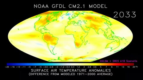
Coupled AOGCMs use transient climate simulations to project/predict climate changes under various scenarios. These can be idealised scenarios (most commonly, CO2 emissions increasing at 1%/yr) or based on recent history (usually the "IS92a" or more recently the SRES scenarios). Which scenarios are most realistic remains uncertain.

The 2001 IPCC Third Assessment Report Figure 9.3 shows the global mean response of 19 different coupled models to an idealised experiment in which emissions increased at 1% per year. Figure 9.5 shows the response of a smaller number of models to more recent trends. For the 7 climate models shown there, the temperature change to 2100 varies from 2 to 4.5 °C with a median of about 3 °C.

Future scenarios do not include unknown events – for example, volcanic eruptions or changes in solar forcing. These effects are believed to be small in comparison to greenhouse gas (GHG) forcing in the long term, but large volcanic eruptions, for example, can exert a substantial temporary cooling effect.

Human GHG emissions are a model input, although it is possible to include an economic/technological submodel to provide these as well. Atmospheric GHG levels are usually supplied as an input, though it is possible to include a carbon cycle model that reflects vegetation and oceanic processes to calculate such levels.

Emissions scenarios

In the 21st century, changes in global mean temperature are projected to vary across the world
Projected change in annual mean surface air temperature from the late 20th century to the middle 21st century, based on SRES emissions scenario A1B (credit: NOAA Geophysical Fluid Dynamics Laboratory).

For the six SRES marker scenarios, IPCC (2007:7–8) gave a "best estimate" of global mean temperature increase (2090–2099 relative to the period 1980–1999) of 1.8 °C to 4.0 °C. Over the same time period, the "likely" range (greater than 66% probability, based on expert judgement) for these scenarios was for a global mean temperature increase of 1.1 to 6.4 °C.

In 2008 a study made climate projections using several emission scenarios. In a scenario where global emissions start to decrease by 2010 and then declined at a sustained rate of 3% per year, the likely global average temperature increase was predicted to be 1.7 °C above pre-industrial levels by 2050, rising to around 2 °C by 2100. In a projection designed to simulate a future where no efforts are made to reduce global emissions, the likely rise in global average temperature was predicted to be 5.5 °C by 2100. A rise as high as 7 °C was thought possible, although less likely.

Another no-reduction scenario resulted in a median warming over land (2090–99 relative to the period 1980–99) of 5.1 °C. Under the same emissions scenario but with a different model, the predicted median warming was 4.1 °C.

Model accuracy

SST errors in HadCM3
 
North American precipitation from various models
 
Temperature predictions from some climate models assuming the SRES A2 emissions scenario

AOGCMs internalise as many processes as are sufficiently understood. However, they are still under development and significant uncertainties remain. They may be coupled to models of other processes in Earth system models, such as the carbon cycle, so as to better model feedbacks. Most recent simulations show "plausible" agreement with the measured temperature anomalies over the past 150 years, when driven by observed changes in greenhouse gases and aerosols. Agreement improves by including both natural and anthropogenic forcings.

Imperfect models may nevertheless produce useful results. GCMs are capable of reproducing the general features of the observed global temperature over the past century.

A debate over how to reconcile climate model predictions that upper air (tropospheric) warming should be greater than observed surface warming, some of which appeared to show otherwise, was resolved in favour of the models, following data revisions.

Cloud effects are a significant area of uncertainty in climate models. Clouds have competing effects on climate. They cool the surface by reflecting sunlight into space; they warm it by increasing the amount of infrared radiation transmitted from the atmosphere to the surface. In the 2001 IPCC report possible changes in cloud cover were highlighted as a major uncertainty in predicting climate.

Climate researchers around the world use climate models to understand the climate system. Thousands of papers have been published about model-based studies. Part of this research is to improve the models.

In 2000, a comparison between measurements and dozens of GCM simulations of ENSO-driven tropical precipitation, water vapor, temperature, and outgoing longwave radiation found similarity between measurements and simulation of most factors. However the simulated change in precipitation was about one-fourth less than what was observed. Errors in simulated precipitation imply errors in other processes, such as errors in the evaporation rate that provides moisture to create precipitation. The other possibility is that the satellite-based measurements are in error. Either indicates progress is required in order to monitor and predict such changes.

The precise magnitude of future changes in climate is still uncertain; for the end of the 21st century (2071 to 2100), for SRES scenario A2, the change of global average SAT change from AOGCMs compared with 1961 to 1990 is +3.0 °C (5.4 °F) and the range is +1.3 to +4.5 °C (+2.3 to 8.1 °F).

The IPCC's Fifth Assessment Report asserted "very high confidence that models reproduce the general features of the global-scale annual mean surface temperature increase over the historical period". However, the report also observed that the rate of warming over the period 1998–2012 was lower than that predicted by 111 out of 114 Coupled Model Intercomparison Project climate models.

Relation to weather forecasting

The global climate models used for climate projections are similar in structure to (and often share computer code with) numerical models for weather prediction, but are nonetheless logically distinct.

Most weather forecasting is done on the basis of interpreting numerical model results. Since forecasts are typically a few days or a week and sea surface temperatures change relatively slowly, such models do not usually contain an ocean model but rely on imposed SSTs. They also require accurate initial conditions to begin the forecast – typically these are taken from the output of a previous forecast, blended with observations. Weather predictions are required at higher temporal resolutions than climate projections, often sub-hourly compared to monthly or yearly averages for climate. However, because weather forecasts only cover around 10 days the models can also be run at higher vertical and horizontal resolutions than climate mode. Currently the ECMWF runs at 9 km (5.6 mi) resolution as opposed to the 100-to-200 km (62-to-124 mi) scale used by typical climate model runs. Often local models are run using global model results for boundary conditions, to achieve higher local resolution: for example, the Met Office runs a mesoscale model with an 11 km (6.8 mi) resolution covering the UK, and various agencies in the US employ models such as the NGM and NAM models. Like most global numerical weather prediction models such as the GFS, global climate models are often spectral models instead of grid models. Spectral models are often used for global models because some computations in modeling can be performed faster, thus reducing run times.

Computations

Climate models use quantitative methods to simulate the interactions of the atmosphere, oceans, land surface and ice.

All climate models take account of incoming energy as short wave electromagnetic radiation, chiefly visible and short-wave (near) infrared, as well as outgoing energy as long wave (far) infrared electromagnetic radiation from the earth. Any imbalance results in a change in temperature.

The most talked-about models of recent years relate temperature to emissions of greenhouse gases. These models project an upward trend in the surface temperature record, as well as a more rapid increase in temperature at higher altitudes.

Three (or more properly, four since time is also considered) dimensional GCM's discretise the equations for fluid motion and energy transfer and integrate these over time. They also contain parametrisations for processes such as convection that occur on scales too small to be resolved directly.

Atmospheric GCMs (AGCMs) model the atmosphere and impose sea surface temperatures as boundary conditions. Coupled atmosphere-ocean GCMs (AOGCMs, e.g. HadCM3, EdGCM, GFDL CM2.X, ARPEGE-Climate) combine the two models.

Models range in complexity:

  • A simple radiant heat transfer model treats the earth as a single point and averages outgoing energy
  • This can be expanded vertically (radiative-convective models), or horizontally
  • Finally, (coupled) atmosphere–ocean–sea ice global climate models discretise and solve the full equations for mass and energy transfer and radiant exchange.
  • Box models treat flows across and within ocean basins.

Other submodels can be interlinked, such as land use, allowing researchers to predict the interaction between climate and ecosystems.

Comparison with other climate models

Earth-system models of intermediate complexity (EMICs)

The Climber-3 model uses a 2.5-dimensional statistical-dynamical model with 7.5° × 22.5° resolution and time step of 1/2 a day. An oceanic submodel is MOM-3 (Modular Ocean Model) with a 3.75° × 3.75° grid and 24 vertical levels.

Radiative-convective models (RCM)

One-dimensional, radiative-convective models were used to verify basic climate assumptions in the 1980s and 1990s.

Earth system models

GCMs can form part of Earth system models, e.g. by coupling ice sheet models for the dynamics of the Greenland and Antarctic ice sheets, and one or more chemical transport models (CTMs) for species important to climate. Thus a carbon chemistry transport model may allow a GCM to better predict anthropogenic changes in carbon dioxide concentrations. In addition, this approach allows accounting for inter-system feedback: e.g. chemistry-climate models allow the effects of climate change on the ozone hole to be studied.

Climate model

From Wikipedia, the free encyclopedia

Climate models are systems of differential equations based on the basic laws of physics, fluid motion, and chemistry. To “run” a model, scientists divide the planet into a 3-dimensional grid, apply the basic equations, and evaluate the results. Atmospheric models calculate winds, heat transfer, radiation, relative humidity, and surface hydrology within each grid and evaluate interactions with neighboring points.

Numerical climate models use quantitative methods to simulate the interactions of the important drivers of climate, including atmosphere, oceans, land surface and ice. They are used for a variety of purposes from study of the dynamics of the climate system to projections of future climate. Climate models may also be qualitative (i.e. not numerical) models and also narratives, largely descriptive, of possible futures.

Quantitative climate models take account of incoming energy from the sun as short wave electromagnetic radiation, chiefly visible and short-wave (near) infrared, as well as outgoing long wave (far) infrared electromagnetic. Any imbalance results in a change in temperature.

Quantitative models vary in complexity:

  • A simple radiant heat transfer model treats the earth as a single point and averages outgoing energy. This can be expanded vertically (radiative-convective models) and/or horizontally
  • Finally, (coupled) atmosphere–ocean–sea ice global climate models solve the full equations for mass and energy transfer and radiant exchange.
  • Other types of modelling can be interlinked, such as land use, in Earth System Models, allowing researchers to predict the interaction between climate and ecosystems.

Box models

Schematic of a simple box model used to illustrate fluxes in geochemical cycles, showing a source (Q), sink (S) and reservoir (M)

Box models are simplified versions of complex systems, reducing them to boxes (or reservoirs) linked by fluxes. The boxes are assumed to be mixed homogeneously. Within a given box, the concentration of any chemical species is therefore uniform. However, the abundance of a species within a given box may vary as a function of time due to the input to (or loss from) the box or due to the production, consumption or decay of this species within the box.

Simple box models, i.e. box model with a small number of boxes whose properties (e.g. their volume) do not change with time, are often useful to derive analytical formulas describing the dynamics and steady-state abundance of a species. More complex box models are usually solved using numerical techniques.

Box models are used extensively to model environmental systems or ecosystems and in studies of ocean circulation and the carbon cycle. They are instances of a multi-compartment model.

Zero-dimensional models

A very simple model of the radiative equilibrium of the Earth is

where

  • the left hand side represents the incoming energy from the Sun
  • the right hand side represents the outgoing energy from the Earth, calculated from the Stefan-Boltzmann law assuming a model-fictive temperature, T, sometimes called the 'equilibrium temperature of the Earth', that is to be found,

and

  • S is the solar constant – the incoming solar radiation per unit area—about 1367 W·m−2
  • is the Earth's average albedo, measured to be 0.3.
  • r is Earth's radius—approximately 6.371×10⁶m
  • π is the mathematical constant (3.141...)
  • is the Stefan-Boltzmann constant—approximately 5.67×10⁻⁸ J·K−4·m−2·s−1
  • is the effective emissivity of earth, about 0.612

The constant πr2 can be factored out, giving

Solving for the temperature,

This yields an apparent effective average earth temperature of 288 K (15 °C; 59 °F). This is because the above equation represents the effective radiative temperature of the Earth (including the clouds and atmosphere).

This very simple model is quite instructive. For example, it easily determines the effect on average earth temperature of changes in solar constant or change of albedo or effective earth emissivity.

The average emissivity of the earth is readily estimated from available data. The emissivities of terrestrial surfaces are all in the range of 0.96 to 0.99 (except for some small desert areas which may be as low as 0.7). Clouds, however, which cover about half of the earth's surface, have an average emissivity of about 0.5 (which must be reduced by the fourth power of the ratio of cloud absolute temperature to average earth absolute temperature) and an average cloud temperature of about 258 K (−15 °C; 5 °F). Taking all this properly into account results in an effective earth emissivity of about 0.64 (earth average temperature 285 K (12 °C; 53 °F)).

This simple model readily determines the effect of changes in solar output or change of earth albedo or effective earth emissivity on average earth temperature. It says nothing, however about what might cause these things to change. Zero-dimensional models do not address the temperature distribution on the earth or the factors that move energy about the earth.

Radiative-convective models

The zero-dimensional model above, using the solar constant and given average earth temperature, determines the effective earth emissivity of long wave radiation emitted to space. This can be refined in the vertical to a one-dimensional radiative-convective model, which considers two processes of energy transport:

  • upwelling and downwelling radiative transfer through atmospheric layers that both absorb and emit infrared radiation
  • upward transport of heat by convection (especially important in the lower troposphere).

The radiative-convective models have advantages over the simple model: they can determine the effects of varying greenhouse gas concentrations on effective emissivity and therefore the surface temperature. But added parameters are needed to determine local emissivity and albedo and address the factors that move energy about the earth.

Effect of ice-albedo feedback on global sensitivity in a one-dimensional radiative-convective climate model.

Higher-dimension models

The zero-dimensional model may be expanded to consider the energy transported horizontally in the atmosphere. This kind of model may well be zonally averaged. This model has the advantage of allowing a rational dependence of local albedo and emissivity on temperature – the poles can be allowed to be icy and the equator warm – but the lack of true dynamics means that horizontal transports have to be specified.

EMICs (Earth-system models of intermediate complexity)

Depending on the nature of questions asked and the pertinent time scales, there are, on the one extreme, conceptual, more inductive models, and, on the other extreme, general circulation models operating at the highest spatial and temporal resolution currently feasible. Models of intermediate complexity bridge the gap. One example is the Climber-3 model. Its atmosphere is a 2.5-dimensional statistical-dynamical model with 7.5° × 22.5° resolution and time step of half a day; the ocean is MOM-3 (Modular Ocean Model) with a 3.75° × 3.75° grid and 24 vertical levels.

GCMs (global climate models or general circulation models)

General Circulation Models (GCMs) discretise the equations for fluid motion and energy transfer and integrate these over time. Unlike simpler models, GCMs divide the atmosphere and/or oceans into grids of discrete "cells", which represent computational units. Unlike simpler models which make mixing assumptions, processes internal to a cell—such as convection—that occur on scales too small to be resolved directly are parameterised at the cell level, while other functions govern the interface between cells.

Atmospheric GCMs (AGCMs) model the atmosphere and impose sea surface temperatures as boundary conditions. Coupled atmosphere-ocean GCMs (AOGCMs, e.g. HadCM3, EdGCM, GFDL CM2.X, ARPEGE-Climat) combine the two models. The first general circulation climate model that combined both oceanic and atmospheric processes was developed in the late 1960s at the NOAA Geophysical Fluid Dynamics Laboratory AOGCMs represent the pinnacle of complexity in climate models and internalise as many processes as possible. However, they are still under development and uncertainties remain. They may be coupled to models of other processes, such as the carbon cycle, so as to better model feedback effects. Such integrated multi-system models are sometimes referred to as either "earth system models" or "global climate models."

Research and development

There are three major types of institution where climate models are developed, implemented and used:

The World Climate Research Programme (WCRP), hosted by the World Meteorological Organization (WMO), coordinates research activities on climate modelling worldwide.

A 2012 U.S. National Research Council report discussed how the large and diverse U.S. climate modeling enterprise could evolve to become more unified. Efficiencies could be gained by developing a common software infrastructure shared by all U.S. climate researchers, and holding an annual climate modeling forum, the report found.

Atmospheric model

From Wikipedia, the free encyclopedia
 
A 96-hour forecast of 850 mbar geopotential height and temperature from the Global Forecast System

An atmospheric model is a mathematical model constructed around the full set of primitive dynamical equations which govern atmospheric motions. It can supplement these equations with parameterizations for turbulent diffusion, radiation, moist processes (clouds and precipitation), heat exchange, soil, vegetation, surface water, the kinematic effects of terrain, and convection. Most atmospheric models are numerical, i.e. they discretize equations of motion. They can predict microscale phenomena such as tornadoes and boundary layer eddies, sub-microscale turbulent flow over buildings, as well as synoptic and global flows. The horizontal domain of a model is either global, covering the entire Earth, or regional (limited-area), covering only part of the Earth. The different types of models run are thermotropic, barotropic, hydrostatic, and nonhydrostatic. Some of the model types make assumptions about the atmosphere which lengthens the time steps used and increases computational speed.

Forecasts are computed using mathematical equations for the physics and dynamics of the atmosphere. These equations are nonlinear and are impossible to solve exactly. Therefore, numerical methods obtain approximate solutions. Different models use different solution methods. Global models often use spectral methods for the horizontal dimensions and finite-difference methods for the vertical dimension, while regional models usually use finite-difference methods in all three dimensions. For specific locations, model output statistics use climate information, output from numerical weather prediction, and current surface weather observations to develop statistical relationships which account for model bias and resolution issues.

Types

The main assumption made by the thermotropic model is that while the magnitude of the thermal wind may change, its direction does not change with respect to height, and thus the baroclinicity in the atmosphere can be simulated using the 500 mb (15 inHg) and 1,000 mb (30 inHg) geopotential height surfaces and the average thermal wind between them.

Barotropic models assume the atmosphere is nearly barotropic, which means that the direction and speed of the geostrophic wind are independent of height. In other words, no vertical wind shear of the geostrophic wind. It also implies that thickness contours (a proxy for temperature) are parallel to upper level height contours. In this type of atmosphere, high and low pressure areas are centers of warm and cold temperature anomalies. Warm-core highs (such as the subtropical ridge and Bermuda-Azores high) and cold-core lows have strengthening winds with height, with the reverse true for cold-core highs (shallow arctic highs) and warm-core lows (such as tropical cyclones). A barotropic model tries to solve a simplified form of atmospheric dynamics based on the assumption that the atmosphere is in geostrophic balance; that is, that the Rossby number of the air in the atmosphere is small. If the assumption is made that the atmosphere is divergence-free, the curl of the Euler equations reduces into the barotropic vorticity equation. This latter equation can be solved over a single layer of the atmosphere. Since the atmosphere at a height of approximately 5.5 kilometres (3.4 mi) is mostly divergence-free, the barotropic model best approximates the state of the atmosphere at a geopotential height corresponding to that altitude, which corresponds to the atmosphere's 500 mb (15 inHg) pressure surface.

Hydrostatic models filter out vertically moving acoustic waves from the vertical momentum equation, which significantly increases the time step used within the model's run. This is known as the hydrostatic approximation. Hydrostatic models use either pressure or sigma-pressure vertical coordinates. Pressure coordinates intersect topography while sigma coordinates follow the contour of the land. Its hydrostatic assumption is reasonable as long as horizontal grid resolution is not small, which is a scale where the hydrostatic assumption fails. Models which use the entire vertical momentum equation are known as nonhydrostatic. A nonhydrostatic model can be solved anelastically, meaning it solves the complete continuity equation for air assuming it is incompressible, or elastically, meaning it solves the complete continuity equation for air and is fully compressible. Nonhydrostatic models use altitude or sigma altitude for their vertical coordinates. Altitude coordinates can intersect land while sigma-altitude coordinates follow the contours of the land.

History

The ENIAC main control panel at the Moore School of Electrical Engineering

The history of numerical weather prediction began in the 1920s through the efforts of Lewis Fry Richardson who utilized procedures developed by Vilhelm Bjerknes. It was not until the advent of the computer and computer simulation that computation time was reduced to less than the forecast period itself. ENIAC created the first computer forecasts in 1950, and more powerful computers later increased the size of initial datasets and included more complicated versions of the equations of motion. In 1966, West Germany and the United States began producing operational forecasts based on primitive-equation models, followed by the United Kingdom in 1972 and Australia in 1977. The development of global forecasting models led to the first climate models. The development of limited area (regional) models facilitated advances in forecasting the tracks of tropical cyclone as well as air quality in the 1970s and 1980s.

Because the output of forecast models based on atmospheric dynamics requires corrections near ground level, model output statistics (MOS) were developed in the 1970s and 1980s for individual forecast points (locations). Even with the increasing power of supercomputers, the forecast skill of numerical weather models only extends to about two weeks into the future, since the density and quality of observations—together with the chaotic nature of the partial differential equations used to calculate the forecast—introduce errors which double every five days. The use of model ensemble forecasts since the 1990s helps to define the forecast uncertainty and extend weather forecasting farther into the future than otherwise possible.

Initialization

A WP-3D Orion weather reconnaissance aircraft in flight

The atmosphere is a fluid. As such, the idea of numerical weather prediction is to sample the state of the fluid at a given time and use the equations of fluid dynamics and thermodynamics to estimate the state of the fluid at some time in the future. On land, terrain maps, available at resolutions down to 1 kilometre (0.62 mi) globally, are used to help model atmospheric circulations within regions of rugged topography, in order to better depict features such as downslope winds, mountain waves, and related cloudiness which affects incoming solar radiation. The main inputs from country-based weather services are surface observations from automated weather stations at ground level over land and from weather buoys at sea. The World Meteorological Organization acts to standardize the instrumentation, observing practices and timing of these observations worldwide. Stations either report hourly in METAR reports, or every six hours in SYNOP reports. Models are initialized using this observed data. The irregularly spaced observations are processed by data assimilation and objective analysis methods, which perform quality control and obtain values at locations usable by the model's mathematical algorithms. The grid used for global models is geodesic or icosahedral, spaced by latitude, longitude, and elevation. The data are then used in the model as the starting point for a forecast.

A variety of methods are used to gather observational data for use in numerical models. Sites launch radiosondes, which rise through the troposphere and well into the stratosphere. Information from weather satellites is used where traditional data sources are not available. Commerce provides pilot reports along aircraft routes and ship reports along shipping routes. Research projects use reconnaissance aircraft to fly in and around weather systems of interest, such as tropical cyclones. Reconnaissance aircraft are also flown over the open oceans during the cold season into systems which cause significant uncertainty in forecast guidance, or are expected to be of high impact 3–7 days into the future over the downstream continent. Sea ice began to be initialized in forecast models in 1971. Efforts to involve sea surface temperature in model initialization began in 1972 due to its role in modulating weather in higher latitudes of the Pacific.

Computation

An example of 500 mbar geopotential height prediction from a numerical weather prediction model.
 
Supercomputers are capable of running highly complex models to help scientists better understand Earth's climate.

A model is a computer program that produces meteorological information for future times at given locations and altitudes. Within any model is a set of equations, known as the primitive equations, used to predict the future state of the atmosphere. These equations are initialized from the analysis data and rates of change are determined. These rates of change predict the state of the atmosphere a short time into the future, with each time increment known as a time step. The equations are then applied to this new atmospheric state to find new rates of change, and these new rates of change predict the atmosphere at a yet further time into the future. Time stepping is repeated until the solution reaches the desired forecast time. The length of the time step chosen within the model is related to the distance between the points on the computational grid, and is chosen to maintain numerical stability. Time steps for global models are on the order of tens of minutes, while time steps for regional models are between one and four minutes. The global models are run at varying times into the future. The UKMET Unified model is run six days into the future, the European Centre for Medium-Range Weather Forecasts model is run out to 10 days into the future, while the Global Forecast System model run by the Environmental Modeling Center is run 16 days into the future.

The equations used are nonlinear partial differential equations which are impossible to solve exactly through analytical methods, with the exception of a few idealized cases. Therefore, numerical methods obtain approximate solutions. Different models use different solution methods: some global models use spectral methods for the horizontal dimensions and finite difference methods for the vertical dimension, while regional models and other global models usually use finite-difference methods in all three dimensions. The visual output produced by a model solution is known as a prognostic chart, or prog.

Parameterization

Weather and climate model gridboxes have sides of between 5 kilometres (3.1 mi) and 300 kilometres (190 mi). A typical cumulus cloud has a scale of less than 1 kilometre (0.62 mi), and would require a grid even finer than this to be represented physically by the equations of fluid motion. Therefore, the processes that such clouds represent are parameterized, by processes of various sophistication. In the earliest models, if a column of air in a model gridbox was unstable (i.e., the bottom warmer than the top) then it would be overturned, and the air in that vertical column mixed. More sophisticated schemes add enhancements, recognizing that only some portions of the box might convect and that entrainment and other processes occur. Weather models that have gridboxes with sides between 5 kilometres (3.1 mi) and 25 kilometres (16 mi) can explicitly represent convective clouds, although they still need to parameterize cloud microphysics. The formation of large-scale (stratus-type) clouds is more physically based, they form when the relative humidity reaches some prescribed value. Still, sub grid scale processes need to be taken into account. Rather than assuming that clouds form at 100% relative humidity, the cloud fraction can be related to a critical relative humidity of 70% for stratus-type clouds, and at or above 80% for cumuliform clouds, reflecting the sub grid scale variation that would occur in the real world.

The amount of solar radiation reaching ground level in rugged terrain, or due to variable cloudiness, is parameterized as this process occurs on the molecular scale. Also, the grid size of the models is large when compared to the actual size and roughness of clouds and topography. Sun angle as well as the impact of multiple cloud layers is taken into account. Soil type, vegetation type, and soil moisture all determine how much radiation goes into warming and how much moisture is drawn up into the adjacent atmosphere. Thus, they are important to parameterize.

Domains

The horizontal domain of a model is either global, covering the entire Earth, or regional, covering only part of the Earth. Regional models also are known as limited-area models, or LAMs. Regional models use finer grid spacing to resolve explicitly smaller-scale meteorological phenomena, since their smaller domain decreases computational demands. Regional models use a compatible global model for initial conditions of the edge of their domain. Uncertainty and errors within LAMs are introduced by the global model used for the boundary conditions of the edge of the regional model, as well as within the creation of the boundary conditions for the LAMs itself.

The vertical coordinate is handled in various ways. Some models, such as Richardson's 1922 model, use geometric height () as the vertical coordinate. Later models substituted the geometric coordinate with a pressure coordinate system, in which the geopotential heights of constant-pressure surfaces become dependent variables, greatly simplifying the primitive equations. This follows since pressure decreases with height through the Earth's atmosphere. The first model used for operational forecasts, the single-layer barotropic model, used a single pressure coordinate at the 500-millibar (15 inHg) level, and thus was essentially two-dimensional. High-resolution models—also called mesoscale models—such as the Weather Research and Forecasting model tend to use normalized pressure coordinates referred to as sigma coordinates.

Global versions

Some of the better known global numerical models are:

Regional versions

Some of the better known regional numerical models are:

  • WRF The Weather Research and Forecasting model was developed cooperatively by NCEP, NCAR, and the meteorological research community. WRF has several configurations, including:
    • WRF-NMM The WRF Nonhydrostatic Mesoscale Model is the primary short-term weather forecast model for the U.S., replacing the Eta model.
    • WRF-ARW Advanced Research WRF developed primarily at the U.S. National Center for Atmospheric Research (NCAR)
  • NAM The term North American Mesoscale model refers to whatever regional model NCEP operates over the North American domain. NCEP began using this designation system in January 2005. Between January 2005 and May 2006 the Eta model used this designation. Beginning in May 2006, NCEP began to use the WRF-NMM as the operational NAM.
  • RAMS the Regional Atmospheric Modeling System developed at Colorado State University for numerical simulations of atmospheric meteorology and other environmental phenomena on scales from meters to hundreds of kilometers – now supported in the public domain
  • MM5 The Fifth Generation Penn State/NCAR Mesoscale Model
  • ARPS the Advanced Region Prediction System developed at the University of Oklahoma is a comprehensive multi-scale nonhydrostatic simulation and prediction system that can be used for regional-scale weather prediction up to the tornado-scale simulation and prediction. Advanced radar data assimilation for thunderstorm prediction is a key part of the system..
  • HIRLAM High Resolution Limited Area Model, is developed by the European NWP research consortia HIRLAM co-funded by 10 European weather services. The meso-scale HIRLAM model is known as HARMONIE and developed in collaboration with Meteo France and ALADIN consortia.
  • GEM-LAM Global Environmental Multiscale Limited Area Model, the high resolution 2.5 km (1.6 mi) GEM by the Meteorological Service of Canada (MSC)
  • ALADIN The high-resolution limited-area hydrostatic and non-hydrostatic model developed and operated by several European and North African countries under the leadership of Météo-France
  • COSMO The COSMO Model, formerly known as LM, aLMo or LAMI, is a limited-area non-hydrostatic model developed within the framework of the Consortium for Small-Scale Modelling (Germany, Switzerland, Italy, Greece, Poland, Romania, and Russia).
  • Meso-NH The Meso-NH Model is a limited-area non-hydrostatic model developed jointly by the Centre National de Recherches Météorologiques and the Laboratoire d'Aérologie (France, Toulouse) since 1998. Its application is from mesoscale to centimetric scales weather simulations.

Model output statistics

Because forecast models based upon the equations for atmospheric dynamics do not perfectly determine weather conditions near the ground, statistical corrections were developed to attempt to resolve this problem. Statistical models were created based upon the three-dimensional fields produced by numerical weather models, surface observations, and the climatological conditions for specific locations. These statistical models are collectively referred to as model output statistics (MOS), and were developed by the National Weather Service for their suite of weather forecasting models. The United States Air Force developed its own set of MOS based upon their dynamical weather model by 1983.

Model output statistics differ from the perfect prog technique, which assumes that the output of numerical weather prediction guidance is perfect. MOS can correct for local effects that cannot be resolved by the model due to insufficient grid resolution, as well as model biases. Forecast parameters within MOS include maximum and minimum temperatures, percentage chance of rain within a several hour period, precipitation amount expected, chance that the precipitation will be frozen in nature, chance for thunderstorms, cloudiness, and surface winds.

Applications

Climate modeling

In 1956, Norman Phillips developed a mathematical model that realistically depicted monthly and seasonal patterns in the troposphere. This was the first successful climate model. Several groups then began working to create general circulation models. The first general circulation climate model combined oceanic and atmospheric processes and was developed in the late 1960s at the Geophysical Fluid Dynamics Laboratory, a component of the U.S. National Oceanic and Atmospheric Administration. By the early 1980s, the U.S. National Center for Atmospheric Research had developed the Community Atmosphere Model (CAM), which can be run by itself or as the atmospheric component of the Community Climate System Model. The latest update (version 3.1) of the standalone CAM was issued on 1 February 2006. In 1986, efforts began to initialize and model soil and vegetation types, resulting in more realistic forecasts. Coupled ocean-atmosphere climate models, such as the Hadley Centre for Climate Prediction and Research's HadCM3 model, are being used as inputs for climate change studies.

Limited area modeling

Model spread with Hurricane Ernesto (2006) within the National Hurricane Center limited area models

Air pollution forecasts depend on atmospheric models to provide fluid flow information for tracking the movement of pollutants. In 1970, a private company in the U.S. developed the regional Urban Airshed Model (UAM), which was used to forecast the effects of air pollution and acid rain. In the mid- to late-1970s, the United States Environmental Protection Agency took over the development of the UAM and then used the results from a regional air pollution study to improve it. Although the UAM was developed for California, it was during the 1980s used elsewhere in North America, Europe, and Asia.

The Movable Fine-Mesh model, which began operating in 1978, was the first tropical cyclone forecast model to be based on atmospheric dynamics. Despite the constantly improving dynamical model guidance made possible by increasing computational power, it was not until the 1980s that numerical weather prediction (NWP) showed skill in forecasting the track of tropical cyclones. And it was not until the 1990s that NWP consistently outperformed statistical or simple dynamical models. Predicting the intensity of tropical cyclones using NWP has also been challenging. As of 2009, dynamical guidance remained less skillful than statistical methods.

Cooperative

From Wikipedia, the free encyclopedia ...