Search This Blog

Saturday, October 8, 2022

Hallmarks of aging

From Wikipedia, the free encyclopedia
https://en.wikipedia.org/wiki/Hallmarks_of_aging

The hallmarks of aging are the types of biochemical changes that occur in all organisms that experience biological aging and lead to a progressive loss of physiological integrity, impaired function and, eventually, death. They were first enumerated in a landmark paper in 2013 to conceptualize the essence of biological aging and its underlying mechanisms.

Overview

The hallmarks of aging

Over time, almost all living organisms experience a gradual and irreversible increase in senescence and an associated loss of proper function of the bodily systems. As aging is the primary risk factor for major human diseases, including cancer, diabetes, cardiovascular disorders, and neurodegenerative diseases, it is important to describe and classify the types of changes that it entails. The nine hallmarks of aging are grouped into three categories as follows:

Primary hallmarks (causes of damage)

Antagonistic hallmarks (responses to damage)

Integrative hallmarks (culprits of the phenotype)

Primary hallmarks are the primary causes of cellular damage. Antagonistic hallmarks are antagonistic or compensatory responses to the manifestation of the primary hallmarks. Integrative hallmarks are the functional result of the previous two groups of hallmarks that lead to further operational deterioration associated with aging.

The hallmarks

Each hallmark was chosen to try to fulfill the following criteria:

  1. manifests during normal aging;
  2. experimentally increasing it accelerates aging;
  3. experimentally amending it slows the normal aging process and increases healthy lifespan.

These conditions are met to different extents by each of these hallmarks. The last criterion is not present in many of the hallmarks, as science has not yet found feasible ways to amend these problems in living organisms.

Genome instability

Proper functioning of the genome is one of the most important prerequisites for the smooth functioning of a cell and the organism as a whole. Alterations in the genetic code have long been considered one of the main causal factors in aging. In multicellular organisms genome instability is central to carcinogenesis, and in humans it is also a factor in some neurodegenerative diseases such as amyotrophic lateral sclerosis or the neuromuscular disease myotonic dystrophy.

Abnormal chemical structures in the DNA are formed mainly through oxidative stress and environmental factors. A number of molecular processes work continuously to repair this damage. Unfortunately, the results are not perfect, and thus damage accumulates over time. Several review articles have shown that deficient DNA repair, allowing greater accumulation of DNA damages, causes premature aging; and that increased DNA repair facilitates greater longevity.

Telomere shortening

Human chromosomes (gray) capped with telomeres (white).

Telomeres are regions of repetitive nucleotide sequences associated with specialized proteins at the ends of linear chromosomes. They protect the terminal regions of chromosomal DNA from progressive degradation and ensure the integrity of linear chromosomes by preventing DNA repair systems from mistaking the ends of the DNA strand for a double strand break.

Telomere shortening is associated with aging, mortality and aging-related diseases. Normal aging is associated with telomere shortening in both humans and mice, and studies on genetically modified animal models suggest causal links between telomere erosion and aging. Leonard Hayflick demonstrated that a normal human fetal cell population will divide between 40 and 60 times in cell culture before entering a senescence phase. Each time a cell undergoes mitosis, the telomeres on the ends of each chromosome shorten slightly. Cell division will cease once telomeres shorten to a critical length. This is useful when uncontrolled cell proliferation (like in cancer) needs to be stopped, but detrimental when normally functioning cells are unable to divide when necessary.

An enzyme called telomerase elongates telomeres in gametes and embryonic stem cells. Telomerase deficiency in humans has been linked to several aging-related diseases related to loss of regenerative capacity of tissues. It has also been shown that premature aging in telomerase-deficient mice is reverted when telomerase is reactivated.

Epigenomic alterations

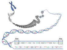
DNA condensation - the DNA chain is wrapped around histones, which form into coils, which wrap into ever larger coils that ultimately make up the chromosome.

Out of all the genes that make up a genome, only a subset are expressed at any given time. The functioning of a genome depends both on the specific order of its nucleotides (genomic factors), and also on which sections of the DNA chain are spooled on histones and thus rendered inaccessible, and which ones are unspooled and available for transcription (epigenomic factors). Depending on the needs of the specific tissue type and environment that a given cell is in, histones can be modified to turn specific genes on or off as needed. The profile of where, when and to what extent these modifications occur (the epigenetic profile) changes with aging, turning useful genes off and unnecessary ones on, disrupting the normal functioning of the cell.

As an example, sirtuins are a type of protein deacetylases that promote the binding of DNA onto histones and thus turn unnecessary genes off. These enzymes use NAD as a cofactor. As we age, the level of NAD in our cells decreases and so does the ability of sirtuins to turn off unneeded genes at the right time. Decreasing the activity of sirtuins has been associated with accelerated aging and increasing their activity has been shown to stave off several age-related diseases.

Loss of proteostasis

Proteostasis is the homeostatic process of maintaining all the proteins necessary for the functioning of the cell in their proper shape, structure and abundance. Protein misfolding, oxidation, abnormal cleavage or undesired post-translational modification can create dysfunctional or even toxic proteins or protein aggregates that hinder the normal functioning of the cell. Though these proteins are continually removed and recycled, formation of damaged or aggregated proteins increases with age, leading to a gradual loss of proteostasis. This can be slowed or suppressed by caloric restriction or by administration of rapamycin, both through inhibiting the mTOR pathway.

Deregulated nutrient sensing

Nutrient sensing is a cell's ability to recognize, and respond to, changes in the concentration of macronutrients such as glucose, fatty acids and amino acids. In times of abundance, anabolism is induced through various pathways, the most well-studied among them the mTOR pathway. When energy and nutrients are scarce, the AMPK receptor senses this and switches off mTOR to conserve resources.

In a growing organism, growth and cell proliferation are important and thus mTOR is upregulated. In a fully grown organism, mTOR-activating signals naturally decline during aging. It has been found that forcibly overactivating these pathways in grown mice leads to accelerated aging and increased incidence of cancer. mTOR inhibition methods like dietary restriction or administering rapamycin have been shown to be one of the most robust methods of increasing lifespan in worms, flies and mice.

Mitochondrial dysfunction

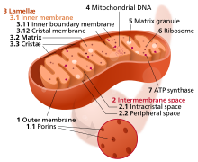
Mitochondrion

The mitochondrion is the powerhouse of the cell. Different human cells contain from 20 to 30 up to several thousand mitochondria, each one converting carbon (in the form of acetyl-CoA) and oxygen into energy (in the form of ATP) and carbon dioxide.

During aging, the efficiency of mitochondria tends to decrease. The reasons for this are still quite unclear, but several mechanisms are suspected - reduced biogenesis, accumulation of damage and mutations in mitochondrial DNA, oxidation of mitochondrial proteins, and defective quality control by mitophagy.

Dysfunctional mitochondria contribute to aging through interfering with intracellular signaling and triggering inflammatory reactions.

Cellular senescence

Under certain conditions, a cell will exit the cell cycle without dying, instead becoming dormant and ceasing its normal function. This is called cellular senescence. Senescence can be induced by several factors, including telomere shortening, DNA damage and stress. Since the immune system is programmed to seek out and eliminate senescent cells, it might be that senescence is one way for the body to rid itself of cells damaged beyond repair.

The links between cell senescence and aging are several:

Stem cell exhaustion

Stem cells are undifferentiated or partially differentiated cells that can proliferate indefinitely. For the first few days after fertilization, the embryo consists almost entirely of stem cells. As the fetus grows, the cells multiply, differentiate and assume their appropriate function within the organism. In adults, stem cells are mostly located in areas that undergo gradual wear (intestine, lung, mucosa, skin) or need continuous replenishment (red blood cells, immune cells, sperm cells, hair follicles).

Loss of regenerative ability is one of the most obvious consequences of aging. This is largely because the proportion of stem cells and the speed of their division gradually lowers over time. It has been found that stem cell rejuvenation can reverse some of the effects of aging at the organismal level.

Altered intercellular communication

Different tissues and the cells they consist of need to orchestrate their work in a tightly controlled manner so that the organism as a whole can function. One of the main ways this is achieved is through excreting signal molecules into the blood where they make their way to other tissues, affecting their behavior. The profile of these molecules changes as we age.

One of the most prominent changes in cell signaling biomarkers is "inflammaging", the development of a chronic low-grade inflammation throughout the body with advanced age. The normal role of inflammation is to recruit the body's immune system and repair mechanisms to a specific damaged area for as long as the damage and threat are present. The constant presence of inflammation markers throughout the body wears out the immune system and damages healthy tissue.

It's also been found that senescent cells excrete a specific set of molecules called the SASP (Senescence-Associated Secretory Phenotype) which induce senescence in neighboring cells. Conversely, lifespan-extending manipulations targeting one tissue can slow the aging process in other tissues as well.

Alternative conceptual models

The Seven Pillars of Aging Model

Other scientists have defined a slightly different conceptual model for aging, called 'The Seven Pillars of Aging', in which just three of the 'hallmarks of aging' are included (stem cells and regeneration, proteostasis, epigenetics). The seven pillars model highlights the interconnectedness between all of the seven pillars which is not highlighted in the nine hallmarks of aging model.

Mass production

From Wikipedia, the free encyclopedia

Mass production, also known as flow production or continuous production, is the production of substantial amounts of standardized products in a constant flow, including and especially on assembly lines. Together with job production and batch production, it is one of the three main production methods.

The term mass production was popularized by a 1926 article in the Encyclopædia Britannica supplement that was written based on correspondence with Ford Motor Company. The New York Times used the term in the title of an article that appeared before publication of the Britannica article.

The concepts of mass production are applied to various kinds of products: from fluids and particulates handled in bulk (food, fuel, chemicals and mined minerals), to parts and assemblies of parts (household appliances and automobiles).

Some mass production techniques, such as standardized sizes and production lines, predate the Industrial Revolution by many centuries; however, it was not until the introduction of machine tools and techniques to produce interchangeable parts were developed in the mid-19th century that modern mass production was possible.

Overview

Mass production involves making many copies of products, very quickly, using assembly line techniques to send partially complete products to workers who each work on an individual step, rather than having a worker work on a whole product from start to finish.

Mass production of fluid matter typically involves pipes with centrifugal pumps or screw conveyors (augers) to transfer raw materials or partially complete products between vessels. Fluid flow processes such as oil refining and bulk materials such as wood chips and pulp are automated using a system of process control which uses various instruments to measure variables such as temperature, pressure, volumetric and level, providing feedback.

Bulk materials such as coal, ores, grains and wood chips are handled by belt, chain, slat, pneumatic or screw conveyors, bucket elevators and mobile equipment such as front-end loaders. Materials on pallets are handled with forklifts. Also used for handling heavy items like reels of paper, steel or machinery are electric overhead cranes, sometimes called bridge cranes because they span large factory bays.

Mass production is capital-intensive and energy-intensive, for it uses a high proportion of machinery and energy in relation to workers. It is also usually automated while total expenditure per unit of product is decreased. However, the machinery that is needed to set up a mass production line (such as robots and machine presses) is so expensive that in order to attain profits there must be some assurance that the product is to be successful to.

One of the descriptions of mass production is that "the skill is built into the tool", which means that the worker using the tool may not need the skill. For example, in the 19th or early 20th century, this could be expressed as "the craftsmanship is in the workbench itself" (not the training of the worker). Rather than having a skilled worker measure every dimension of each part of the product against the plans or the other parts as it is being formed, there were jigs ready at hand to ensure that the part was made to fit this set-up. It had already been checked that the finished part would be to specifications to fit all the other finished parts—and it would be made more quickly, with no time spent on finishing the parts to fit one another. Later, once computerized control came about (for example, CNC), jigs were obviated, but it remained true that the skill (or knowledge) was built into the tool (or process, or documentation) rather than residing in the worker's head. This is the specialized capital required for mass production; each workbench and set of tools (or each CNC cell, or each fractionating column) is different (fine-tuned to its task).

History

Pre-industrial

Sometimes production in series has obvious benefits, as is the case with this 5-sickle casting mold from the Bronze Age on show at a museum in Yekaterinburg, Russia.
 
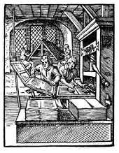
This woodcut from 1568 shows the left printer removing a page from the press while the one at right inks the text-blocks. Such a duo could reach 14,000 hand movements per working day, printing around 3,600 pages in the process.

Standardized parts and sizes and factory production techniques were developed in pre-industrial times; before the invention of machine tools the manufacture of precision parts, especially metal ones, was very labor-intensive.

Crossbows made with bronze parts were produced in China during the Warring States period. The Qin Emperor unified China at least in part by equipping large armies with these weapons, which were equipped with a sophisticated trigger mechanism made of interchangeable parts. The Terracotta Army guarding the Emperor's necropolis is also believed to have been created through the use of standardized molds on an assembly line.

In ancient Carthage, ships of war were mass-produced on a large scale at a moderate cost, allowing them to efficiently maintain their control of the Mediterranean. Many centuries later, the Republic of Venice would follow Carthage in producing ships with prefabricated parts on an assembly line: the Venetian Arsenal produced nearly one ship every day in what was effectively the world's first factory, which at its height employed 16,000 people.

The invention of movable type has allowed for documents such as books to be mass produced. The first movable type system was invented in China by Bi Sheng, during the reign of the Song Dynasty, where it was used to, among other things, issue paper money. The oldest extant book produced using metal type is the Jikji, printed in Korea in the year 1377. Johannes Gutenberg, through his invention of the printing press and production of the Gutenberg Bible, introduced movable type to Europe. Through this introduction, mass production in the European publishing industry was made commonplace, leading to a democratization of knowledge, increased literacy and education, and the beginnings of modern science.

Jean-Baptiste de Gribeauval, a French artillery engineer, introduced the standardization of cannon design in the mid-18th century. He developed a 6-inch (150 mm) field howitzer whose gun barrel, carriage assembly and ammunition specifications were made uniform for all French cannons. The standardized interchangeable parts of these cannons down to the nuts, bolts and screws made their mass production and repair easier than before.

Industrial

In the Industrial Revolution, simple mass production techniques were used at the Portsmouth Block Mills in England to make ships' pulley blocks for the Royal Navy in the Napoleonic Wars. It was achieved in 1803 by Marc Isambard Brunel in cooperation with Henry Maudslay under the management of Sir Samuel Bentham. The first unmistakable examples of manufacturing operations carefully designed to reduce production costs by specialized labour and the use of machines appeared in the 18th century in England.

A pulley block for rigging on a sailing ship. By 1808, annual production in Portsmouth reached 130,000 blocks.

The Navy was in a state of expansion that required 100,000 pulley blocks to be manufactured a year. Bentham had already achieved remarkable efficiency at the docks by introducing power-driven machinery and reorganising the dockyard system. Brunel, a pioneering engineer, and Maudslay, a pioneer of machine tool technology who had developed the first industrially practical screw-cutting lathe in 1800 which standardized screw thread sizes for the first time which in turn allowed the application of interchangeable parts, collaborated on plans to manufacture block-making machinery. By 1805, the dockyard had been fully updated with the revolutionary, purpose-built machinery at a time when products were still built individually with different components. A total of 45 machines were required to perform 22 processes on the blocks, which could be made into one of three possible sizes. The machines were almost entirely made of metal thus improving their accuracy and durability. The machines would make markings and indentations on the blocks to ensure alignment throughout the process. One of the many advantages of this new method was the increase in labour productivity due to the less labour-intensive requirements of managing the machinery. Richard Beamish, assistant to Brunel's son and engineer, Isambard Kingdom Brunel, wrote:

So that ten men, by the aid of this machinery, can accomplish with uniformity, celerity and ease, what formerly required the uncertain labour of one hundred and ten.

By 1808, annual production from the 45 machines had reached 130,000 blocks and some of the equipment was still in operation as late as the mid-twentieth century. Mass production techniques were also used to rather limited extent to make clocks and watches, and to make small arms, though parts were usually non-interchangeable. Though produced on a very small scale, Crimean War gunboat engines designed and assembled by John Penn of Greenwich are recorded as the first instance of the application of mass production techniques (though not necessarily the assembly-line method) to marine engineering. In filling an Admiralty order for 90 sets to his high-pressure and high-revolution horizontal trunk engine design, Penn produced them all in 90 days. He also used Whitworth Standard threads throughout. Prerequisites for the wide use of mass production were interchangeable parts, machine tools and power, especially in the form of electricity.

Some of the organizational management concepts needed to create 20th-century mass production, such as scientific management, had been pioneered by other engineers (most of whom are not famous, but Frederick Winslow Taylor is one of the well-known ones), whose work would later be synthesized into fields such as industrial engineering, manufacturing engineering, operations research, and management consultancy. Although after leaving the Henry Ford Company which was rebranded as Cadillac and later was awarded the Dewar Trophy in 1908 for creating interchangeable mass-produced precision engine parts, Henry Ford downplayed the role of Taylorism in the development of mass production at his company. However, Ford management performed time studies and experiments to mechanize their factory processes, focusing on minimizing worker movements. The difference is that while Taylor focused mostly on efficiency of the worker, Ford also substituted for labor by using machines, thoughtfully arranged, wherever possible.

In 1807, Eli Terry was hired to produce 4,000 wooden movement clocks in the Porter Contract. At this time, the annual yield for wooden clocks did not exceed a few dozen on average. Terry developed a Milling machine in 1795, in which he perfected Interchangeable parts. In 1807, Terry developed a spindle cutting machine, which could produce multiple parts at the same time. Terry hired Silas Hoadley and Seth Thomas to work the Assembly line at the facilities. The Porter Contract was the first contract which called for mass production of clock movements in history. In 1815, Terry began mass-producing the first shelf clock. Chauncey Jerome, an apprentice of Eli Terry mass-produced up to 20,000 brass clocks annually in 1840 when he invented the cheap 30-hour OG clock.

The United States Department of War sponsored the development of interchangeable parts for guns produced at the arsenals at Springfield, Massachusetts and Harpers Ferry, Virginia (now West Virginia) in the early decades of the 19th century, finally achieving reliable interchangeability by about 1850. This period coincided with the development of machine tools, with the armories designing and building many of their own. Some of the methods employed were a system of gauges for checking dimensions of the various parts and jigs and fixtures for guiding the machine tools and properly holding and aligning the work pieces. This system came to be known as armory practice or the American system of manufacturing, which spread throughout New England aided by skilled mechanics from the armories who were instrumental in transferring the technology to the sewing machines manufacturers and other industries such as machine tools, harvesting machines and bicycles. Singer Manufacturing Co., at one time the largest sewing machine manufacturer, did not achieve interchangeable parts until the late 1880s, around the same time Cyrus McCormick adopted modern manufacturing practices in making harvesting machines.

Mass production of Consolidated B-32 Dominator airplanes at Consolidated Aircraft Plant No. 4, near Fort Worth, Texas, during World War II.

During World War II, The United States mass-produced many vehicles and weapons, such as ships (i.e. Liberty Ships, Higgins boats ), aircraft (i.e. North American P-51 Mustang, Consolidated B-24 Liberator, Boeing B-29 Superfortress), jeeps (i.e. Willys MB), trucks, tanks (i.e. M4 Sherman) and M2 Browning and M1919 Browning machine guns. Many vehicles, transported by ships have been shipped in parts and later assembled on-site.

For the ongoing energy transition, many wind turbine components and solar panels are being mass-produced. Wind turbines and solar panels are being used in respectively wind farms and solar farms.

In addition, in the ongoing climate change mitigation, large-scale carbon sequestration (through reforestation, blue carbon restoration, etc) has been proposed. Some projects (such as the Trillion Tree Campaign) involve planting a very large amount of trees. In order to speed up such efforts, fast propagation of trees may be useful. Some automated machines have been produced to allow for fast (vegetative) plant propagation. Also, for some plants that help to sequester carbon (such as seagrass), techniques have been developed to help speed up the process.

Mass production benefited from the development of materials such as inexpensive steel, high strength steel and plastics. Machining of metals was greatly enhanced with high-speed steel and later very hard materials such as tungsten carbide for cutting edges. Fabrication using steel components was aided by the development of electric welding and stamped steel parts, both which appeared in industry in about 1890. Plastics such as polyethylene, polystyrene and polyvinyl chloride (PVC) can be easily formed into shapes by extrusion, blow molding or injection molding, resulting in very low cost manufacture of consumer products, plastic piping, containers and parts.

An influential article that helped to frame and popularize the 20th century's definition of mass production appeared in a 1926 Encyclopædia Britannica supplement. The article was written based on correspondence with Ford Motor Company and is sometimes credited as the first use of the term.

Factory electrification

Electrification of factories began very gradually in the 1890s after the introduction of a practical DC motor by Frank J. Sprague and accelerated after the AC motor was developed by Galileo Ferraris, Nikola Tesla and Westinghouse, Mikhail Dolivo-Dobrovolsky and others. Electrification of factories was fastest between 1900 and 1930, aided by the establishment of electric utilities with central stations and the lowering of electricity prices from 1914 to 1917.

Electric motors were several times more efficient than small steam engines because central station generation were more efficient than small steam engines and because line shafts and belts had high friction losses. Electric motors also allowed more flexibility in manufacturing and required less maintenance than line shafts and belts. Many factories saw a 30% increase in output simply from changing over to electric motors.

Electrification enabled modern mass production, as with Thomas Edison's iron ore processing plant (about 1893) that could process 20,000 tons of ore per day with two shifts, each of five men. At that time it was still common to handle bulk materials with shovels, wheelbarrows and small narrow-gauge rail cars, and for comparison, a canal digger in previous decades typically handled five tons per 12-hour day.

The biggest impact of early mass production was in manufacturing everyday items, such as at the Ball Brothers Glass Manufacturing Company, which electrified its mason jar plant in Muncie, Indiana, U.S., around 1900. The new automated process used glass-blowing machines to replace 210 craftsman glass blowers and helpers. A small electric truck was used to handle 150 dozen bottles at a time where previously a hand truck would carry six dozen. Electric mixers replaced men with shovels handling sand and other ingredients that were fed into the glass furnace. An electric overhead crane replaced 36 day laborers for moving heavy loads across the factory.

According to Henry Ford:

The provision of a whole new system of electric generation emancipated industry from the leather belt and line shaft, for it eventually became possible to provide each tool with its own electric motor. This may seem only a detail of minor importance. In fact, modern industry could not be carried out with the belt and line shaft for a number of reasons. The motor enabled machinery to be arranged in the order of the work, and that alone has probably doubled the efficiency of industry, for it has cut out a tremendous amount of useless handling and hauling. The belt and line shaft were also tremendously wasteful – so wasteful indeed that no factory could be really large, for even the longest line shaft was small according to modern requirements. Also high speed tools were impossible under the old conditions – neither the pulleys nor the belts could stand modern speeds. Without high speed tools and the finer steels which they brought about, there could be nothing of what we call modern industry.

The assembly plant of the Bell Aircraft Corporation in 1944. Note parts of overhead crane at both sides of photo near top.

Mass production was popularized in the late 1910s and 1920s by Henry Ford's Ford Motor Company, which introduced electric motors to the then-well-known technique of chain or sequential production. Ford also bought or designed and built special purpose machine tools and fixtures such as multiple spindle drill presses that could drill every hole on one side of an engine block in one operation and a multiple head milling machine that could simultaneously machine 15 engine blocks held on a single fixture. All of these machine tools were arranged systematically in the production flow and some had special carriages for rolling heavy items into machining position. Production of the Ford Model T used 32,000 machine tools.

Buildings

The process of prefabrication, wherein parts are created separately from the finished product, is at the core of all mass-produced construction. Early examples include movable structures reportedly utilized by Akbar the Great, and the chattel houses built by emancipated slaves on Barbados. The Nissen hut, first used by the British during World War I, married prefabrication and mass production in a way that suited the needs of the military. The simple structures, which cost little and could be erected in just a couple of hours, were highly successful: over 100,000 Nissen huts were produced during World War I alone, and they would go on to serve in other conflicts and inspire a number of similar designs.

Following World War II, in the United States, William Levitt pioneered the building of standardized tract houses in 56 different locations around the country. These communities were dubbed Levittowns, and they were able to be constructed quickly and cheaply through the leveraging of economies of scale, as well as the specialization of construction tasks in a process akin to an assembly line. This era also saw the invention of the mobile home, a small prefabricated house that can be transported cheaply on a truck bed.

In the modern industrialization of construction, mass production is often used for prefabrication of house components.

The use of assembly lines

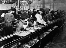
Ford assembly line, 1913. The magneto assembly line was the first.

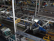
Mass production systems for items made of numerous parts are usually organized into assembly lines. The assemblies pass by on a conveyor, or if they are heavy, hung from an overhead crane or monorail.

In a factory for a complex product, rather than one assembly line, there may be many auxiliary assembly lines feeding sub-assemblies (i.e. car engines or seats) to a backbone "main" assembly line. A diagram of a typical mass-production factory looks more like the skeleton of a fish than a single line.

Vertical integration

Vertical integration is a business practice that involves gaining complete control over a product's production, from raw materials to final assembly.

In the age of mass production, this caused shipping and trade problems in that shipping systems were unable to transport huge volumes of finished automobiles (in Henry Ford's case) without causing damage, and also government policies imposed trade barriers on finished units.

Ford built the Ford River Rouge Complex with the idea of making the company's own iron and steel in the same large factory site where parts and car assembly took place. River Rouge also generated its own electricity.

Upstream vertical integration, such as to raw materials, is away from leading technology toward mature, low-return industries. Most companies chose to focus on their core business rather than vertical integration. This included buying parts from outside suppliers, who could often produce them as cheaply or cheaper.

Standard Oil, the major oil company in the 19th century, was vertically integrated partly because there was no demand for unrefined crude oil, but kerosene and some other products were in great demand. The other reason was that Standard Oil monopolized the oil industry. The major oil companies were, and many still are, vertically integrated, from production to refining and with their own retail stations, although some sold off their retail operations. Some oil companies also have chemical divisions.

Lumber and paper companies at one time owned most of their timber lands and sold some finished products such as corrugated boxes. The tendency has been to divest of timber lands to raise cash and to avoid property taxes.

Advantages and disadvantages

The economies of mass production come from several sources. The primary cause is a reduction of non-productive effort of all types. In craft production, the craftsman must bustle about a shop, getting parts and assembling them. He must locate and use many tools many times for varying tasks. In mass production, each worker repeats one or a few related tasks that use the same tool to perform identical or near-identical operations on a stream of products. The exact tool and parts are always at hand, having been moved down the assembly line consecutively. The worker spends little or no time retrieving and/or preparing materials and tools, and so the time taken to manufacture a product using mass production is shorter than when using traditional methods.

The probability of human error and variation is also reduced, as tasks are predominantly carried out by machinery; error in operating such machinery has more far-reaching consequences. A reduction in labour costs, as well as an increased rate of production, enables a company to produce a larger quantity of one product at a lower cost than using traditional, non-linear methods.

However, mass production is inflexible because it is difficult to alter a design or production process after a production line is implemented. Also, all products produced on one production line will be identical or very similar, and introducing variety to satisfy individual tastes is not easy. However, some variety can be achieved by applying different finishes and decorations at the end of the production line if necessary. The starter cost for the machinery can be expensive so the producer must be sure it sells or the producers will lose a lot of money.

The Ford Model T produced tremendous affordable output but was not very good at responding to demand for variety, customization, or design changes. As a consequence Ford eventually lost market share to General Motors, who introduced annual model changes, more accessories and a choice of colors.

With each passing decade, engineers have found ways to increase the flexibility of mass production systems, driving down the lead times on new product development and allowing greater customization and variety of products.

Compared with other production methods, mass production can create new occupational hazards for workers. This is partly due to the need for workers to operate heavy machinery while also working close together with many other workers. Preventative safety measures, such as fire drills, as well as special training is therefore necessary to minimise the occurrence of industrial accidents.

Socioeconomic impacts

In the 1830s, French political thinker and historian Alexis de Tocqueville identified one of the key characteristics of America that would later make it so amenable to the development of mass production: the homogeneous consumer base. De Tocqueville wrote in his Democracy in America (1835) that "The absence in the United States of those vast accumulations of wealth which favor the expenditures of large sums on articles of mere luxury... impact to the productions of American industry a character distinct from that of other countries' industries. [Production is geared toward] articles suited to the wants of the whole people".

Mass production improved productivity, which was a contributing factor to economic growth and the decline in work week hours, alongside other factors such as transportation infrastructures (canals, railroads and highways) and agricultural mechanization. These factors caused the typical work week to decline from 70 hours in the early 19th century to 60 hours late in the century, then to 50 hours in the early 20th century and finally to 40 hours in the mid-1930s.

Mass production permitted great increases in total production. Using a European crafts system into the late 19th century it was difficult to meet demand for products such as sewing machines and animal powered mechanical harvesters. By the late 1920s many previously scarce goods were in good supply. One economist has argued that this constituted "overproduction" and contributed to high unemployment during the Great Depression. Say's law denies the possibility of general overproduction and for this reason classical economists deny that it had any role in the Great Depression.

Mass production allowed the evolution of consumerism by lowering the unit cost of many goods used.

Reinforcement learning

From Wikipedia, the free encyclopedia

Reinforcement learning (RL) is an area of machine learning concerned with how intelligent agents ought to take actions in an environment in order to maximize the notion of cumulative reward. Reinforcement learning is one of three basic machine learning paradigms, alongside supervised learning and unsupervised learning.

Reinforcement learning differs from supervised learning in not needing labelled input/output pairs be presented, and in not needing sub-optimal actions to be explicitly corrected. Instead the focus is on finding a balance between exploration (of uncharted territory) and exploitation (of current knowledge). Partially supervised RL algorithms can combine the advantages of supervised and RL algorithms.

The environment is typically stated in the form of a Markov decision process (MDP), because many reinforcement learning algorithms for this context use dynamic programming techniques. The main difference between the classical dynamic programming methods and reinforcement learning algorithms is that the latter do not assume knowledge of an exact mathematical model of the MDP and they target large MDPs where exact methods become infeasible.

Introduction

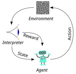
The typical framing of a Reinforcement Learning (RL) scenario: an agent takes actions in an environment, which is interpreted into a reward and a representation of the state, which are fed back into the agent.

Due to its generality, reinforcement learning is studied in many disciplines, such as game theory, control theory, operations research, information theory, simulation-based optimization, multi-agent systems, swarm intelligence, and statistics. In the operations research and control literature, reinforcement learning is called approximate dynamic programming, or neuro-dynamic programming. The problems of interest in reinforcement learning have also been studied in the theory of optimal control, which is concerned mostly with the existence and characterization of optimal solutions, and algorithms for their exact computation, and less with learning or approximation, particularly in the absence of a mathematical model of the environment. In economics and game theory, reinforcement learning may be used to explain how equilibrium may arise under bounded rationality.

Basic reinforcement learning is modeled as a Markov decision process (MDP):

  • a set of environment and agent states, S;
  • a set of actions, A, of the agent;
  • is the probability of transition (at time ) from state to state under action .
  • is the immediate reward after transition from to with action .

The purpose of reinforcement learning is for the agent to learn an optimal, or nearly-optimal, policy that maximizes the "reward function" or other user-provided reinforcement signal that accumulates from the immediate rewards. This is similar to processes that appear to occur in animal psychology. For example, biological brains are hardwired to interpret signals such as pain and hunger as negative reinforcements, and interpret pleasure and food intake as positive reinforcements. In some circumstances, animals can learn to engage in behaviors that optimize these rewards. This suggests that animals are capable of reinforcement learning.

A basic reinforcement learning agent AI interacts with its environment in discrete time steps. At each time t, the agent receives the current state and reward . It then chooses an action from the set of available actions, which is subsequently sent to the environment. The environment moves to a new state and the reward associated with the transition is determined. The goal of a reinforcement learning agent is to learn a policy: , which maximizes the expected cumulative reward.

Formulating the problem as an MDP assumes the agent directly observes the current environmental state; in this case the problem is said to have full observability. If the agent only has access to a subset of states, or if the observed states are corrupted by noise, the agent is said to have partial observability, and formally the problem must be formulated as a Partially observable Markov decision process. In both cases, the set of actions available to the agent can be restricted. For example, the state of an account balance could be restricted to be positive; if the current value of the state is 3 and the state transition attempts to reduce the value by 4, the transition will not be allowed.

When the agent's performance is compared to that of an agent that acts optimally, the difference in performance gives rise to the notion of regret. In order to act near optimally, the agent must reason about the long-term consequences of its actions (i.e., maximize future income), although the immediate reward associated with this might be negative.

Thus, reinforcement learning is particularly well-suited to problems that include a long-term versus short-term reward trade-off. It has been applied successfully to various problems, including robot control, elevator scheduling, telecommunications, backgammon, checkers and Go (AlphaGo).

Two elements make reinforcement learning powerful: the use of samples to optimize performance and the use of function approximation to deal with large environments. Thanks to these two key components, reinforcement learning can be used in large environments in the following situations:

  • A model of the environment is known, but an analytic solution is not available;
  • Only a simulation model of the environment is given (the subject of simulation-based optimization);
  • The only way to collect information about the environment is to interact with it.

The first two of these problems could be considered planning problems (since some form of model is available), while the last one could be considered to be a genuine learning problem. However, reinforcement learning converts both planning problems to machine learning problems.

Exploration

The exploration vs. exploitation trade-off has been most thoroughly studied through the multi-armed bandit problem and for finite state space MDPs in Burnetas and Katehakis (1997).

Reinforcement learning requires clever exploration mechanisms; randomly selecting actions, without reference to an estimated probability distribution, shows poor performance. The case of (small) finite MDPs is relatively well understood. However, due to the lack of algorithms that scale well with the number of states (or scale to problems with infinite state spaces), simple exploration methods are the most practical.

One such method is -greedy, where is a parameter controlling the amount of exploration vs. exploitation. With probability , exploitation is chosen, and the agent chooses the action that it believes has the best long-term effect (ties between actions are broken uniformly at random). Alternatively, with probability , exploration is chosen, and the action is chosen uniformly at random. is usually a fixed parameter but can be adjusted either according to a schedule (making the agent explore progressively less), or adaptively based on heuristics.

Algorithms for control learning

Even if the issue of exploration is disregarded and even if the state was observable (assumed hereafter), the problem remains to use past experience to find out which actions lead to higher cumulative rewards.

Criterion of optimality

Policy

The agent's action selection is modeled as a map called policy:

The policy map gives the probability of taking action when in state . There are also deterministic policies.

State-value function

The value function is defined as the expected return starting with state , i.e. , and successively following policy . Hence, roughly speaking, the value function estimates "how good" it is to be in a given state.

where the random variable denotes the return, and is defined as the sum of future discounted rewards:

where is the reward at step , is the discount-rate. Gamma is less than 1, so events in the distant future are weighted less than events in the immediate future.

The algorithm must find a policy with maximum expected return. From the theory of MDPs it is known that, without loss of generality, the search can be restricted to the set of so-called stationary policies. A policy is stationary if the action-distribution returned by it depends only on the last state visited (from the observation agent's history). The search can be further restricted to deterministic stationary policies. A deterministic stationary policy deterministically selects actions based on the current state. Since any such policy can be identified with a mapping from the set of states to the set of actions, these policies can be identified with such mappings with no loss of generality.

Brute force

The brute force approach entails two steps:

  • For each possible policy, sample returns while following it
  • Choose the policy with the largest expected return

One problem with this is that the number of policies can be large, or even infinite. Another is that the variance of the returns may be large, which requires many samples to accurately estimate the return of each policy.

These problems can be ameliorated if we assume some structure and allow samples generated from one policy to influence the estimates made for others. The two main approaches for achieving this are value function estimation and direct policy search.

Value function

Value function approaches attempt to find a policy that maximizes the return by maintaining a set of estimates of expected returns for some policy (usually either the "current" [on-policy] or the optimal [off-policy] one).

These methods rely on the theory of Markov decision processes, where optimality is defined in a sense that is stronger than the above one: A policy is called optimal if it achieves the best-expected return from any initial state (i.e., initial distributions play no role in this definition). Again, an optimal policy can always be found amongst stationary policies.

To define optimality in a formal manner, define the value of a policy by

where stands for the return associated with following from the initial state . Defining as the maximum possible value of , where is allowed to change,

A policy that achieves these optimal values in each state is called optimal. Clearly, a policy that is optimal in this strong sense is also optimal in the sense that it maximizes the expected return , since , where is a state randomly sampled from the distribution of initial states (so ).

Although state-values suffice to define optimality, it is useful to define action-values. Given a state , an action and a policy , the action-value of the pair under is defined by

where now stands for the random return associated with first taking action in state and following , thereafter.

The theory of MDPs states that if is an optimal policy, we act optimally (take the optimal action) by choosing the action from with the highest value at each state, . The action-value function of such an optimal policy () is called the optimal action-value function and is commonly denoted by . In summary, the knowledge of the optimal action-value function alone suffices to know how to act optimally.

Assuming full knowledge of the MDP, the two basic approaches to compute the optimal action-value function are value iteration and policy iteration. Both algorithms compute a sequence of functions () that converge to . Computing these functions involves computing expectations over the whole state-space, which is impractical for all but the smallest (finite) MDPs. In reinforcement learning methods, expectations are approximated by averaging over samples and using function approximation techniques to cope with the need to represent value functions over large state-action spaces.

Monte Carlo methods

Monte Carlo methods can be used in an algorithm that mimics policy iteration. Policy iteration consists of two steps: policy evaluation and policy improvement.

Monte Carlo is used in the policy evaluation step. In this step, given a stationary, deterministic policy , the goal is to compute the function values (or a good approximation to them) for all state-action pairs . Assume (for simplicity) that the MDP is finite, that sufficient memory is available to accommodate the action-values and that the problem is episodic and after each episode a new one starts from some random initial state. Then, the estimate of the value of a given state-action pair can be computed by averaging the sampled returns that originated from over time. Given sufficient time, this procedure can thus construct a precise estimate of the action-value function . This finishes the description of the policy evaluation step.

In the policy improvement step, the next policy is obtained by computing a greedy policy with respect to : Given a state , this new policy returns an action that maximizes . In practice lazy evaluation can defer the computation of the maximizing actions to when they are needed.

Problems with this procedure include:

1. The procedure may spend too much time evaluating a suboptimal policy.

2. It uses samples inefficiently in that a long trajectory improves the estimate only of the single state-action pair that started the trajectory.

3. When the returns along the trajectories have high variance, convergence is slow.

4. It works in episodic problems only.

5. It works in small, finite MDPs only.

Temporal difference methods

The first problem is corrected by allowing the procedure to change the policy (at some or all states) before the values settle. This too may be problematic as it might prevent convergence. Most current algorithms do this, giving rise to the class of generalized policy iteration algorithms. Many actor-critic methods belong to this category.

The second issue can be corrected by allowing trajectories to contribute to any state-action pair in them. This may also help to some extent with the third problem, although a better solution when returns have high variance is Sutton's temporal difference (TD) methods that are based on the recursive Bellman equation. The computation in TD methods can be incremental (when after each transition the memory is changed and the transition is thrown away), or batch (when the transitions are batched and the estimates are computed once based on the batch). Batch methods, such as the least-squares temporal difference method, may use the information in the samples better, while incremental methods are the only choice when batch methods are infeasible due to their high computational or memory complexity. Some methods try to combine the two approaches. Methods based on temporal differences also overcome the fourth issue.

Another problem specific to TD comes from their reliance on the recursive Bellman equation. Most TD methods have a so-called parameter that can continuously interpolate between Monte Carlo methods that do not rely on the Bellman equations and the basic TD methods that rely entirely on the Bellman equations. This can be effective in palliating this issue.

Function approximation methods

In order to address the fifth issue, function approximation methods are used. Linear function approximation starts with a mapping that assigns a finite-dimensional vector to each state-action pair. Then, the action values of a state-action pair are obtained by linearly combining the components of with some weights :

The algorithms then adjust the weights, instead of adjusting the values associated with the individual state-action pairs. Methods based on ideas from nonparametric statistics (which can be seen to construct their own features) have been explored.

Value iteration can also be used as a starting point, giving rise to the Q-learning algorithm and its many variants.

The problem with using action-values is that they may need highly precise estimates of the competing action values that can be hard to obtain when the returns are noisy, though this problem is mitigated to some extent by temporal difference methods. Using the so-called compatible function approximation method compromises generality and efficiency.

Direct policy search

An alternative method is to search directly in (some subset of) the policy space, in which case the problem becomes a case of stochastic optimization. The two approaches available are gradient-based and gradient-free methods.

Gradient-based methods (policy gradient methods) start with a mapping from a finite-dimensional (parameter) space to the space of policies: given the parameter vector , let denote the policy associated to . Defining the performance function by

under mild conditions this function will be differentiable as a function of the parameter vector . If the gradient of was known, one could use gradient ascent. Since an analytic expression for the gradient is not available, only a noisy estimate is available. Such an estimate can be constructed in many ways, giving rise to algorithms such as Williams' REINFORCE method (which is known as the likelihood ratio method in the simulation-based optimization literature). Policy search methods have been used in the robotics context. Many policy search methods may get stuck in local optima (as they are based on local search).

A large class of methods avoids relying on gradient information. These include simulated annealing, cross-entropy search or methods of evolutionary computation. Many gradient-free methods can achieve (in theory and in the limit) a global optimum.

Policy search methods may converge slowly given noisy data. For example, this happens in episodic problems when the trajectories are long and the variance of the returns is large. Value-function based methods that rely on temporal differences might help in this case. In recent years, actor–critic methods have been proposed and performed well on various problems.

Model-based algorithms

Finally, all of the above methods can be combined with algorithms that first learn a model. For instance, the Dyna algorithm learns a model from experience, and uses that to provide more modelled transitions for a value function, in addition to the real transitions. Such methods can sometimes be extended to use of non-parametric models, such as when the transitions are simply stored and 'replayed' to the learning algorithm.

There are other ways to use models than to update a value function. For instance, in model predictive control the model is used to update the behavior directly.

Theory

Both the asymptotic and finite-sample behaviors of most algorithms are well understood. Algorithms with provably good online performance (addressing the exploration issue) are known.

Efficient exploration of MDPs is given in Burnetas and Katehakis (1997). Finite-time performance bounds have also appeared for many algorithms, but these bounds are expected to be rather loose and thus more work is needed to better understand the relative advantages and limitations.

For incremental algorithms, asymptotic convergence issues have been settled. Temporal-difference-based algorithms converge under a wider set of conditions than was previously possible (for example, when used with arbitrary, smooth function approximation).

Research

Research topics include

  • adaptive methods that work with fewer (or no) parameters under a large number of conditions
  • addressing the exploration problem in large MDPs
  • combinations with logic-based frameworks
  • large-scale empirical evaluations
  • learning and acting under partial information (e.g., using predictive state representation)
  • modular and hierarchical reinforcement learning
  • improving existing value-function and policy search methods
  • algorithms that work well with large (or continuous) action spaces
  • transfer learning
  • lifelong learning
  • efficient sample-based planning (e.g., based on Monte Carlo tree search).
  • bug detection in software projects
  • Intrinsic motivation which differentiates information-seeking, curiosity-type behaviours from task-dependent goal-directed behaviours (typically) by introducing a reward function based on maximising novel information
  • Multiagent or distributed reinforcement learning is a topic of interest. Applications are expanding.
  • Actor-critic reinforcement learning
  • Reinforcement learning algorithms such as TD learning are under investigation as a model for dopamine-based learning in the brain. In this model, the dopaminergic projections from the substantia nigra to the basal ganglia function as the prediction error.
  • Reinforcement learning has been used as a part of the model for human skill learning, especially in relation to the interaction between implicit and explicit learning in skill acquisition (the first publication on this application was in 1995–1996).
  • Occupant-centric control
  • Algorithmic trading and optimal execution
  • Optimization of computing resources

Comparison of reinforcement learning algorithms

Algorithm Description Policy Action Space State Space Operator
Monte Carlo Every visit to Monte Carlo Either Discrete Discrete Sample-means
Q-learning State–action–reward–state Off-policy Discrete Discrete Q-value
SARSA State–action–reward–state–action On-policy Discrete Discrete Q-value
Q-learning - Lambda State–action–reward–state with eligibility traces Off-policy Discrete Discrete Q-value
SARSA - Lambda State–action–reward–state–action with eligibility traces On-policy Discrete Discrete Q-value
DQN Deep Q Network Off-policy Discrete Continuous Q-value
DDPG Deep Deterministic Policy Gradient Off-policy Continuous Continuous Q-value
A3C Asynchronous Advantage Actor-Critic Algorithm On-policy Continuous Continuous Advantage
NAF Q-Learning with Normalized Advantage Functions Off-policy Continuous Continuous Advantage
TRPO Trust Region Policy Optimization On-policy Continuous Continuous Advantage
PPO Proximal Policy Optimization On-policy Continuous Continuous Advantage
TD3 Twin Delayed Deep Deterministic Policy Gradient Off-policy Continuous Continuous Q-value
SAC Soft Actor-Critic Off-policy Continuous Continuous Advantage

Associative reinforcement learning

Associative reinforcement learning tasks combine facets of stochastic learning automata tasks and supervised learning pattern classification tasks. In associative reinforcement learning tasks, the learning system interacts in a closed loop with its environment.

Deep reinforcement learning

This approach extends reinforcement learning by using a deep neural network and without explicitly designing the state space. The work on learning ATARI games by Google DeepMind increased attention to deep reinforcement learning or end-to-end reinforcement learning.

Adversarial deep reinforcement learning

Adversarial deep reinforcement learning is an active area of research in reinforcement learning focusing on vulnerabilities of learned policies. In this research area some studies initially showed that reinforcement learning policies are susceptible to imperceptible adversarial manipulations. While some methods have been proposed to overcome these susceptibilities, in the most recent studies it has been shown that these proposed solutions are far from providing an accurate representation of current vulnerabilities of deep reinforcement learning policies.

Fuzzy reinforcement learning

By introducing fuzzy inference in RL, approximating the state-action value function with fuzzy rules in continuous space becomes possible. The IF - THEN form of fuzzy rules make this approach suitable for expressing the results in a form close to natural language. Extending FRL with Fuzzy Rule Interpolation  allows the use of reduced size sparse fuzzy rule-bases to emphasize cardinal rules (most important state-action values).

Inverse reinforcement learning

In inverse reinforcement learning (IRL), no reward function is given. Instead, the reward function is inferred given an observed behavior from an expert. The idea is to mimic observed behavior, which is often optimal or close to optimal.

Safe reinforcement learning

Safe reinforcement learning (SRL) can be defined as the process of learning policies that maximize the expectation of the return in problems in which it is important to ensure reasonable system performance and/or respect safety constraints during the learning and/or deployment processes.

Partially supervised reinforcement learning (PSRL)

In PSRL algorithms the advantages of supervised and RL based approaches are synergistically combined. For example the control policy learnt by an inverse ANN based approach to control a nonlinear system can be refined using RL thereby avoiding the computational cost incurred by starting from a random policy in traditional RL. Partially supervised approaches can alleviate the need for extensive training data in supervised learning while reducing the need for costly exhaustive random exploration in pure RL.

Common Gateway Interface

From Wikipedia, the free encyclopedia https://en.wikipedia.org/wiki/Com...