Translation (biology)

From Wikipedia, the free encyclopedia
https://en.wikipedia.org/wiki/Translation_(biology)

Overview of the translation of eukaryotic messenger RNA

 

Diagram showing the translation of mRNA and the synthesis of proteins by a ribosome

 

Initiation and elongation stages of translation as seen through zooming in on the nitrogenous bases in RNA, the ribosome, the tRNA, and amino acids, with short explanations.

 

The three phases of translation initiation polymerase bind to the DNA strand and move along until the small ribosomal subunit binds to the DNA. Elongation is initiated when the large subunit attaches and termination ends the process of elongation.

In molecular biology and genetics, translation is the process in which ribosomes in the cytoplasm or endoplasmic reticulum synthesize proteins after the process of transcription of DNA to RNA in the cell's nucleus. The entire process is called gene expression.

In translation, messenger RNA (mRNA) is decoded in a ribosome, outside the nucleus, to produce a specific amino acid chain, or polypeptide. The polypeptide later folds into an active protein and performs its functions in the cell. The ribosome facilitates decoding by inducing the binding of complementary tRNA anticodon sequences to mRNA codons. The tRNAs carry specific amino acids that are chained together into a polypeptide as the mRNA passes through and is "read" by the ribosome.

Translation proceeds in three phases:

1. Initiation: The ribosome assembles around the target mRNA. The first tRNA is attached at the start codon.
2. Elongation: The last tRNA validated by the small ribosomal subunit (accommodation) transfers the amino acid. It carries to the large ribosomal subunit which binds it to the one of the preceding admitted tRNA (transpeptidation). The ribosome then moves to the next mRNA codon to continue the process (translocation), creating an amino acid chain.
3. Termination: When a stop codon is reached, the ribosome releases the polypeptide. The ribosomal complex remains intact and moves on to the next mRNA to be translated.

In prokaryotes (bacteria and archaea), translation occurs in the cytosol, where the large and small subunits of the ribosome bind to the mRNA. In eukaryotes, translation occurs in the cytoplasm or across the membrane of the endoplasmic reticulum in a process called co-translational translocation. In co-translational translocation, the entire ribosome/mRNA complex binds to the outer membrane of the rough endoplasmic reticulum (ER), and the new protein is synthesized and released into the ER; the newly created polypeptide can be stored inside the ER for future vesicle transport and secretion outside the cell, or immediately secreted.

Many types of transcribed RNA, such as transfer RNA, ribosomal RNA, and small nuclear RNA, do not undergo a translation into proteins.

Several antibiotics act by inhibiting translation. These include anisomycin, cycloheximide, chloramphenicol, tetracycline, streptomycin, erythromycin, and puromycin. Prokaryotic ribosomes have a different structure from that of eukaryotic ribosomes, and thus antibiotics can specifically target bacterial infections without any harm to a eukaryotic host's cells.

Basic mechanisms

Further information: Bacterial translation, Archaeal translation, and Eukaryotic translation

 

A ribosome translating a protein that is secreted into the endoplasmic reticulum. tRNAs are colored dark blue.

 

Tertiary structure of tRNA. CCA tail in yellow, Acceptor stem in purple, Variable loop in orange, D arm in red, Anticodon arm in blue with Anticodon in black, T arm in green.

The basic process of protein production is the addition of one amino acid at a time to the end of a protein. This operation is performed by a ribosome. A ribosome is made up of two subunits, a small subunit, and a large subunit. These subunits come together before the translation of mRNA into a protein to provide a location for translation to be carried out and a polypeptide to be produced. The choice of amino acid type to add is determined by an mRNA molecule. Each amino acid added is matched to a three-nucleotide subsequence of the mRNA. For each such triplet possible, the corresponding amino acid is accepted. The successive amino acids added to the chain are matched to successive nucleotide triplets in the mRNA. In this way, the sequence of nucleotides in the template mRNA chain determines the sequence of amino acids in the generated amino acid chain. The addition of an amino acid occurs at the C-terminus of the peptide; thus, translation is said to be amine-to-carboxyl directed.

The mRNA carries genetic information encoded as a ribonucleotide sequence from the chromosomes to the ribosomes. The ribonucleotides are "read" by translational machinery in a sequence of nucleotide triplets called codons. Each of those triplets codes for a specific amino acid.

The ribosome molecules translate this code to a specific sequence of amino acids. The ribosome is a multisubunit structure containing rRNA and proteins. It is the "factory" where amino acids are assembled into proteins. tRNAs are small noncoding RNA chains (74–93 nucleotides) that transport amino acids to the ribosome. The repertoire of tRNA genes varies widely between species, with some Bacteria having between 20 and 30 genes while complex eukaryotes could have thousands. tRNAs have a site for amino acid attachment, and a site called an anticodon. The anticodon is an RNA triplet complementary to the mRNA triplet that codes for their cargo amino acid.

Aminoacyl tRNA synthetases (enzymes) catalyze the bonding between specific tRNAs and the amino acids that their anticodon sequences call for. The product of this reaction is an aminoacyl-tRNA. In bacteria, this aminoacyl-tRNA is carried to the ribosome by EF-Tu, where mRNA codons are matched through complementary base pairing to specific tRNA anticodons. Aminoacyl-tRNA synthetases that mispair tRNAs with the wrong amino acids can produce mischarged aminoacyl-tRNAs, which can result in inappropriate amino acids at the respective position in the protein. This "mistranslation" of the genetic code naturally occurs at low levels in most organisms, but certain cellular environments cause an increase in permissive mRNA decoding, sometimes to the benefit of the cell.

The ribosome has two binding sites for tRNA. They are the aminoacyl site (abbreviated A), and the peptidyl site/ exit site (abbreviated P/E). Concerning the mRNA, the three sites are oriented 5’ to 3’ E-P-A, because ribosomes move toward the 3' end of mRNA. The A-site binds the incoming tRNA with the complementary codon on the mRNA. The P/E-site holds the tRNA with the growing polypeptide chain. When an aminoacyl-tRNA initially binds to its corresponding codon on the mRNA, it is in the A site. Then, a peptide bond forms between the amino acid of the tRNA in the A site and the amino acid of the charged tRNA in the P/E site. The growing polypeptide chain is transferred to the tRNA in the A site. Translocation occurs, moving the tRNA to the P/E site, now without an amino acid; the tRNA that was in the A site, now charged with the polypeptide chain, is moved to the P/E site and the tRNA leaves, and nothinger aminoacyl-tRNA enters the A site to repeat the process.

After the new amino acid is added to the chain, and after the tRNA is released out of the ribosome and into the cytosol, the energy provided by the hydrolysis of a GTP bound to the translocase EF-G (in bacteria) and a/eEF-2 (in eukaryotes and archaea) moves the ribosome down one codon towards the 3' end. The energy required for translation of proteins is significant. For a protein containing n amino acids, the number of high-energy phosphate bonds required to translate it is 4n-1. The rate of translation varies; it is significantly higher in prokaryotic cells (up to 17–21 amino acid residues per second) than in eukaryotic cells (up to 6–9 amino acid residues per second).

Even though the ribosomes are usually considered accurate and processive machines, the translation process is subject to errors that can lead either to the synthesis of erroneous proteins or to the premature abandonment of translation, either because a tRNA couples to a wrong codon or because a tRNA is coupled to the wrong amino acid. The rate of error in synthesizing proteins has been estimated to be between 1 in 10⁵ and 1 in 10³ misincorporated amino acids, depending on the experimental conditions. The rate of premature translation abandonment, instead, has been estimated to be of the order of magnitude of 10⁻⁴ events per translated codon. The correct amino acid is covalently bonded to the correct transfer RNA (tRNA) by amino acyl transferases. The amino acid is joined by its carboxyl group to the 3' OH of the tRNA by an ester bond. When the tRNA has an amino acid linked to it, the tRNA is termed "charged". Initiation involves the small subunit of the ribosome binding to the 5' end of mRNA with the help of initiation factors (IF). In bacteria and a minority of archaea, initiation of protein synthesis involves the recognition of a purine-rich initiation sequence on the mRNA called the Shine-Dalgarno sequence. The Shine-Dalgarno sequence binds to a complementary pyrimidine-rich sequence on the 3' end of the 16S rRNA part of the 30S ribosomal subunit. The binding of these complementary sequences ensures that the 30S ribosomal subunit is bound to the mRNA and is aligned such that the initiation codon is placed in the 30S portion of the P-site. Once the mRNA and 30S subunit are properly bound, an initiation factor brings the initiator tRNA-amino acid complex, f-Met-tRNA, to the 30S P site. The initiation phase is completed once a 50S subunit joins the 30 subunit, forming an active 70S ribosome. Termination of the polypeptide occurs when the A site of the ribosome is occupied by a stop codon (UAA, UAG, or UGA) on the mRNA, creating the primary structure of a protein. tRNA usually cannot recognize or bind to stop codons. Instead, the stop codon induces the binding of a release factor protein (RF1 & RF2) that prompts the disassembly of the entire ribosome/mRNA complex by the hydrolysis of the polypeptide chain from the peptidyl transferase center of the ribosome. Drugs or special sequence motifs on the mRNA can change the ribosomal structure so that near-cognate tRNAs are bound to the stop codon instead of the release factors. In such cases of 'translational readthrough', translation continues until the ribosome encounters the next stop codon.

The process of translation is highly regulated in both eukaryotic and prokaryotic organisms. Regulation of translation can impact the global rate of protein synthesis which is closely coupled to the metabolic and proliferative state of a cell. In addition, recent work has revealed that genetic differences and their subsequent expression as mRNAs can also impact translation rate in an RNA-specific manner.

Clinical significance

Translational control is critical for the development and survival of cancer. Cancer cells must frequently regulate the translation phase of gene expression, though it is not fully understood why translation is targeted over steps like transcription. While cancer cells often have genetically altered translation factors, it is much more common for cancer cells to modify the levels of existing translation factors. Several major oncogenic signaling pathways, including the RAS–MAPK, PI3K/AKT/mTOR, MYC, and WNT–β-catenin pathways, ultimately reprogram the genome via translation. Cancer cells also control translation to adapt to cellular stress. During stress, the cell translates mRNAs that can mitigate the stress and promote survival. An example of this is the expression of AMPK in various cancers; its activation triggers a cascade that can ultimately allow the cancer to escape apoptosis (programmed cell death) triggered by nutrition deprivation. Future cancer therapies may involve disrupting the translation machinery of the cell to counter the downstream effects of cancer.

Mathematical modeling of translation

Figure M0. Basic and the simplest model M0 of protein synthesis. Here, *M – amount of mRNA with translation initiation site not occupied by assembling ribosome, *F – amount of mRNA with translation initiation site occupied by assembling ribosome, *R – amount of ribosomes sitting on mRNA synthesizing proteins, *P – amount of synthesized proteins.

 

Figure M1'. The extended model of protein synthesis M1 with explicit presentation of 40S, 60S and initiation factors (IF) binding.

The transcription-translation process description, mentioning only the most basic ”elementary” processes, consists of:

1. production of mRNA molecules (including splicing),
2. initiation of these molecules with help of initiation factors (e.g., the initiation can include the circularization step though it is not universally required),
3. initiation of translation, recruiting the small ribosomal subunit,
4. assembly of full ribosomes,
5. elongation, (i.e. movement of ribosomes along mRNA with production of protein),
6. termination of translation,
7. degradation of mRNA molecules,
8. degradation of proteins.

The process of amino acid building to create protein in translation is a subject of various physic models for a long time starting from the first detailed kinetic models such as or others taking into account stochastic aspects of translation and using computer simulations. Many chemical kinetics-based models of protein synthesis have been developed and analyzed in the last four decades. Beyond chemical kinetics, various modeling formalisms such as Totally Asymmetric Simple Exclusion Process (TASEP),^[23]Probabilistic Boolean Networks (PBN), Petri Nets and max-plus algebra have been applied to model the detailed kinetics of protein synthesis or some of its stages. A basic model of protein synthesis that takes into account all eight 'elementary' processes has been developed, following the paradigm that "useful models are simple and extendable". The simplest model M0 is represented by the reaction kinetic mechanism (Figure M0). It was generalised to include 40S, 60S and initiation factors (IF) binding (Figure M1'). It was extended further to include effect of microRNA on protein synthesis. Most of models in this hierarchy can be solved analytically. These solutions were used to extract 'kinetic signatures' of different specific mechanisms of synthesis regulation.

Genetic code

Main article: Genetic code

It is also possible to translate either by hand (for short sequences) or by computer (after first programming one appropriately, see section below); this allows biologists and chemists to draw out the chemical structure of the encoded protein on paper.

First, convert each template DNA base to its RNA complement (note that the complement of A is now U), as shown below. Note that the template strand of the DNA is the one the RNA is polymerized against; the other DNA strand would be the same as the RNA, but with thymine instead of uracil.

DNA -> RNA
 A  ->  U
 T  ->  A
 C  ->  G
 G  ->  C
 A=T-> A=U

Then split the RNA into triplets (groups of three bases). Note that there are 3 translation "windows", or reading frames, depending on where you start reading the code. Finally, use the table at Genetic code to translate the above into a structural formula as used in chemistry.

This will give you the primary structure of the protein. However, proteins tend to fold, depending in part on hydrophilic and hydrophobic segments along the chain. Secondary structure can often still be guessed at, but the proper tertiary structure is often very hard to determine.

Whereas other aspects such as the 3D structure, called tertiary structure, of protein can only be predicted using sophisticated algorithms, the amino acid sequence, called primary structure, can be determined solely from the nucleic acid sequence with the aid of a translation table.

This approach may not give the correct amino acid composition of the protein, in particular if unconventional amino acids such as selenocysteine are incorporated into the protein, which is coded for by a conventional stop codon in combination with a downstream hairpin (SElenoCysteine Insertion Sequence, or SECIS).

There are many computer programs capable of translating a DNA/RNA sequence into a protein sequence. Normally this is performed using the Standard Genetic Code, however, few programs can handle all the "special" cases, such as the use of the alternative initiation codons which are biologically significant. For instance, the rare alternative start codon CTG codes for Methionine when used as a start codon, and for Leucine in all other positions.

Example: Condensed translation table for the Standard Genetic Code (from the NCBI Taxonomy webpage).

 AAs    = FFLLSSSSYY**CC*WLLLLPPPPHHQQRRRRIIIMTTTTNNKKSSRRVVVVAAAADDEEGGGG
 Starts = ---M---------------M---------------M----------------------------
 Base1  = TTTTTTTTTTTTTTTTCCCCCCCCCCCCCCCCAAAAAAAAAAAAAAAAGGGGGGGGGGGGGGGG
 Base2  = TTTTCCCCAAAAGGGGTTTTCCCCAAAAGGGGTTTTCCCCAAAAGGGGTTTTCCCCAAAAGGGG
 Base3  = TCAGTCAGTCAGTCAGTCAGTCAGTCAGTCAGTCAGTCAGTCAGTCAGTCAGTCAGTCAGTCAG

The "Starts" row indicate three start codons, UUG, CUG, and the very common AUG. It also indicates the first amino acid residue when interpreted as a start: in this case it is all methionine.

Translation tables

Main articles: List of genetic codes and Genetic code § List of alternative codons

Even when working with ordinary eukaryotic sequences such as the Yeast genome, it is often desired to be able to use alternative translation tables—namely for translation of the mitochondrial genes. Currently the following translation tables are defined by the NCBI Taxonomy Group for the translation of the sequences in GenBank:

1. The standard code
2. The vertebrate mitochondrial code
3. The yeast mitochondrial code
4. The mold, protozoan, and coelenterate mitochondrial code and the mycoplasma/spiroplasma code
5. The invertebrate mitochondrial code
6. The ciliate, dasycladacean and hexamita nuclear code
7. The kinetoplast code
9. The echinoderm and flatworm mitochondrial code
10. The euplotid nuclear code
11. The bacterial, archaeal and plant plastid code
12. The alternative yeast nuclear code
13. The ascidian mitochondrial code
14. The alternative flatworm mitochondrial code
15. The Blepharisma nuclear code
16. The chlorophycean mitochondrial code
21. The trematode mitochondrial code
22. The Scenedesmus obliquus mitochondrial code
23. The Thraustochytrium mitochondrial code
24. The Pterobranchia mitochondrial code
25. The candidate division SR1 and gracilibacteria code
26. The Pachysolen tannophilus nuclear code
27. The karyorelict nuclear code
28. The Condylostoma nuclear code
29. The Mesodinium nuclear code
30. The peritrich nuclear code
31. The Blastocrithidia nuclear code
33. The Cephalodiscidae mitochondrial code

Opioid peptide

From Wikipedia, the free encyclopedia

https://en.wikipedia.org/wiki/Opioid_peptide 

 

Vertebrate endogenous opioids neuropeptide
Identifiers
Symbol	Opiods_neuropep
Pfam	PF01160
InterPro	IPR006024
PROSITE	PDOC00964

Available protein structures:

Structural correlation between met-enkephalin, an opioid peptide, (left) and morphine, an opiate drug, (right)

Opioid peptides or opiate peptides are peptides that bind to opioid receptors in the brain; opiates and opioids mimic the effect of these peptides. Such peptides may be produced by the body itself, for example endorphins. The effects of these peptides vary, but they all resemble those of opiates. Brain opioid peptide systems are known to play an important role in motivation, emotion, attachment behaviour, the response to stress and pain, control of food intake, and the rewarding effects of alcohol and nicotine.

Opioid-like peptides may also be absorbed from partially digested food (casomorphins, exorphins, and rubiscolins). Opioid peptides from food typically have lengths between 4–8 amino acids. Endogenous opioids are generally much longer.

Opioid peptides are released by post-translational proteolytic cleavage of precursor proteins. The precursors consist of the following components: a signal sequence that precedes a conserved region of about 50 residues; a variable-length region; and the sequence of the neuropeptides themselves. Sequence analysis reveals that the conserved N-terminal region of the precursors contains 6 cysteines, which are probably involved in disulfide bond formation. It is speculated that this region might be important for neuropeptide processing.

Endogenous

The human genome contains several homologous genes that are known to code for endogenous opioid peptides.

• The nucleotide sequence of the human gene for proopiomelanocortin (POMC) was characterized in 1980. The POMC gene codes for endogenous opioids such as β-endorphin and γ-endorphin.
• The human gene for the enkephalins was isolated and its sequence described in 1982.
• The human gene for dynorphins (originally called the "Enkephalin B" gene because of sequence similarity to the enkephalin gene) was isolated and its sequence described in 1983.
• The PNOC gene encoding prepronociceptin, which is cleaved into nociceptin and potentially two additional neuropeptides.
• Adrenorphin, amidorphin, and leumorphin were discovered in the 1980s.
• The endomorphins were discovered in the 1990s.
• Opiorphin and spinorphin, enkephalinase inhibitors (i.e., prevent the metabolism of enkephalins).
• Hemorphins, hemoglobin-derived opioid peptides, including hemorphin-4, valorphin, and spinorphin, among others.

While not peptides, codeine and morphine are also produced in the human body.

Exogenous

Exogenous opioid substances are called exorphins, as opposed to endorphins. Exorphins include opioid food peptides like Gluten exorphin and opioid food peptides and are mostly contained in cereals and animal milk. Exorphins mimic the actions of endorphins by binding to an activating opioid receptors in the brain.

Common exorphins include:

• Casomorphin (from casein found in milk of mammals, including cows)
• Gluten exorphin (from gluten found in cereals wheat, rye, barley)
• Gliadorphin/gluteomorphin (from gluten found in cereals wheat, rye, barley)
• Soymorphin-5 (from soybean)
• Rubiscolin (from spinach)

Amphibian

• Deltorphin
• Deltorphin I
• Deltorphin II
• Dermorphin

Synthetic

• Zyklophin – semisynthetic KOR antagonist derived from dynorphin A

Peptide

From Wikipedia, the free encyclopedia

https://en.wikipedia.org/wiki/Peptide

 

A tetrapeptide (example Val-Gly-Ser-Ala) with green marked amino end (L-valine) and
blue marked carboxyl end (L-alanine)

Peptides are short chains of amino acids linked by peptide bonds. A polypeptide is a longer, continuous, unbranched peptide chain. Polypeptides which have a molecular mass of 10,000 Da or more are called proteins. Chains of fewer than twenty amino acids are called oligopeptides, and include dipeptides, tripeptides, and tetrapeptides.

Peptides fall under the broad chemical classes of biological polymers and oligomers, alongside nucleic acids, oligosaccharides, polysaccharides, and others.

Proteins consist of one or more polypeptides arranged in a biologically functional way, often bound to ligands such as coenzymes and cofactors, to another protein or other macromolecule such as DNA or RNA, or to complex macromolecular assemblies.

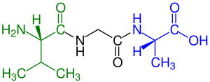
Amino acids that have been incorporated into peptides are termed residues. A water molecule is released during formation of each amide bond. All peptides except cyclic peptides have an N-terminal (amine group) and C-terminal (carboxyl group) residue at the end of the peptide (as shown for the tetrapeptide in the image).

Classes

There are numerous types of peptides that have been classified according to their sources and functions. According to the Handbook of Biologically Active Peptides, some groups of peptides include plant peptides, bacterial/antibiotic peptides, fungal peptides, invertebrate peptides, amphibian/skin peptides, venom peptides, cancer/anticancer peptides, vaccine peptides, immune/inflammatory peptides, brain peptides, endocrine peptides, ingestive peptides, gastrointestinal peptides, cardiovascular peptides, renal peptides, respiratory peptides, opioid peptides, neurotrophic peptides, and blood–brain peptides.

Some ribosomal peptides are subject to proteolysis. These function, typically in higher organisms, as hormones and signaling molecules. Some microbes produce peptides as antibiotics, such as microcins and bacteriocins.

Peptides frequently have post-translational modifications such as phosphorylation, hydroxylation, sulfonation, palmitoylation, glycosylation, and disulfide formation. In general, peptides are linear, although lariat structures have been observed. More exotic manipulations do occur, such as racemization of L-amino acids to D-amino acids in platypus venom.

Nonribosomal peptides are assembled by enzymes, not the ribosome. A common non-ribosomal peptide is glutathione, a component of the antioxidant defenses of most aerobic organisms. Other nonribosomal peptides are most common in unicellular organisms, plants, and fungi and are synthesized by modular enzyme complexes called nonribosomal peptide synthetases.

These complexes are often laid out in a similar fashion, and they can contain many different modules to perform a diverse set of chemical manipulations on the developing product. These peptides are often cyclic and can have highly complex cyclic structures, although linear nonribosomal peptides are also common. Since the system is closely related to the machinery for building fatty acids and polyketides, hybrid compounds are often found. The presence of oxazoles or thiazoles often indicates that the compound was synthesized in this fashion.

Peptones are derived from animal milk or meat digested by proteolysis. In addition to containing small peptides, the resulting material includes fats, metals, salts, vitamins, and many other biological compounds. Peptones are used in nutrient media for growing bacteria and fungi.

Peptide fragments refer to fragments of proteins that are used to identify or quantify the source protein. Often these are the products of enzymatic degradation performed in the laboratory on a controlled sample, but can also be forensic or paleontological samples that have been degraded by natural effects.

Chemical synthesis

Main article: Peptide synthesis

 

Solid-phase peptide synthesis on a rink amide resin using Fmoc-α-amine-protected amino acid

Protein-peptide interactions

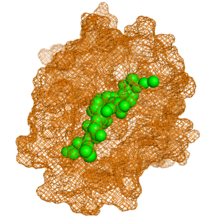
Example of a protein (orange) and peptide (green) interaction. Obtained from Propedia: a peptide-protein interactions database.

Peptides can perform interactions with proteins and other macromolecules. They are responsible for several important function in human cells, such as cell signaling and act as immune modulators. Indeed, studies have reported that 15-40% of all protein-protein interactions in human cells are mediated by peptides. Additionally, it is estimated that at least 10% of pharmaceutical market is based on peptides products.

Example families

The peptide families in this section are ribosomal peptides, usually with hormonal activity. All of these peptides are synthesized by cells as longer "propeptides" or "proproteins" and truncated prior to exiting the cell. They are released into the bloodstream where they perform their signaling functions.

Antimicrobial peptides

• Magainin family
• Cecropin family
• Cathelicidin family
• Defensin family

Tachykinin peptides

Main article: Tachykinin peptides

• Substance P
• Kassinin
• Neurokinin A
• Eledoisin
• Neurokinin B

Vasoactive intestinal peptides

Main article: Secretin family

• VIP (Vasoactive Intestinal Peptide; PHM27)
• PACAP Pituitary Adenylate Cyclase Activating Peptide
• Peptide PHI 27 (Peptide Histidine Isoleucine 27)
• GHRH 1-24 (Growth Hormone Releasing Hormone 1-24)
• Glucagon
• Secretin

Pancreatic polypeptide-related peptides

• NPY (NeuroPeptide Y)
• PYY (Peptide YY)
• APP (Avian Pancreatic Polypeptide)
• PPY Pancreatic PolYpeptide

Opioid peptides

Main article: Opioid peptide

• Proopiomelanocortin (POMC) peptides
• Enkephalin pentapeptides
• Prodynorphin peptides

Calcitonin peptides

• Calcitonin
• Amylin
• AGG01

Self-assembling peptides

• Aromatic short peptides
• Biomimetic peptides
• Peptide amphiphiles
• Peptide dendrimers

Other peptides

• B-type Natriuretic Peptide (BNP) - produced in the myocardium and useful in medical diagnosis
• Lactotripeptides - Lactotripeptides might reduce blood pressure, although the evidence is mixed.
• Peptidic components from traditional Chinese medicine Colla Corii Asini in hematopoiesis.

Terminology

Length

Several terms related to peptides have no strict length definitions, and there is often overlap in their usage:

• A polypeptide is a single linear chain of many amino acids (any length), held together by amide bonds.
• A protein consists of one or more polypeptides (more than about 50 amino acids long).
• An oligopeptide consists of only a few amino acids (between two and twenty).

Number of amino acids

A tripeptide (example Val-Gly-Ala) with green marked amino end (L-valine) and blue marked  carboxyl end (L-alanine)

Peptides and proteins are often described by the number of amino acids in their chain, e.g. a protein with 158 amino acids may be described as a "158 amino-acid-long protein". Peptides of specific shorter lengths are named using IUPAC numerical multiplier prefixes:

• A monopeptide has one amino acid.
• A dipeptide has two amino acids.
• A tripeptide has three amino acids.
• A tetrapeptide has four amino acids.
• A pentapeptide has five amino acids. (e.g., enkephalin).
• A hexapeptide has six amino acids. (e.g., angiotensin IV).
• A heptapeptide has seven amino acids. (e.g., spinorphin).
• An octapeptide has eight amino acids (e.g., angiotensin II).
• A nonapeptide has nine amino acids (e.g., oxytocin).
• A decapeptide has ten amino acids (e.g., gonadotropin-releasing hormone and angiotensin I).
• A undecapeptide has eleven amino acids (e.g., substance P).

The same words are also used to describe a group of residues in a larger polypeptide (e.g., RGD motif).

Function

• A neuropeptide is a peptide that is active in association with neural tissue.
• A lipopeptide is a peptide that has a lipid connected to it, and pepducins are lipopeptides that interact with GPCRs.
• A peptide hormone is a peptide that acts as a hormone.
• A proteose is a mixture of peptides produced by the hydrolysis of proteins. The term is somewhat archaic.
• A peptidergic agent (or drug) is a chemical which functions to directly modulate the peptide systems in the body or brain. An example is opioidergics, which are neuropeptidergics.
• A cell-penetrating peptide is a peptide able to penetrate the cell membrane.

Correlation

From Wikipedia, the free encyclopedia

https://en.wikipedia.org/wiki/Correlation

 

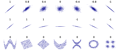
Several sets of (x, y) points, with the Pearson correlation coefficient of x and y for each set. The correlation reflects the noisiness and direction of a linear relationship (top row), but not the slope of that relationship (middle), nor many aspects of nonlinear relationships (bottom). N.B.: the figure in the center has a slope of 0 but in that case, the correlation coefficient is undefined because the variance of Y is zero.

In statistics, correlation or dependence is any statistical relationship, whether causal or not, between two random variables or bivariate data. Although in the broadest sense, "correlation" may indicate any type of association, in statistics it usually refers to the degree to which a pair of variables are linearly related. Familiar examples of dependent phenomena include the correlation between the height of parents and their offspring, and the correlation between the price of a good and the quantity the consumers are willing to purchase, as it is depicted in the so-called demand curve.

Correlations are useful because they can indicate a predictive relationship that can be exploited in practice. For example, an electrical utility may produce less power on a mild day based on the correlation between electricity demand and weather. In this example, there is a causal relationship, because extreme weather causes people to use more electricity for heating or cooling. However, in general, the presence of a correlation is not sufficient to infer the presence of a causal relationship (i.e., correlation does not imply causation).

Formally, random variables are dependent if they do not satisfy a mathematical property of probabilistic independence. In informal parlance, correlation is synonymous with dependence. However, when used in a technical sense, correlation refers to any of several specific types of mathematical operations between the tested variables and their respective expected values. Essentially, correlation is the measure of how two or more variables are related to one another. There are several correlation coefficients, often denoted ${\displaystyle \rho }$ or ${\displaystyle r}$, measuring the degree of correlation. The most common of these is the Pearson correlation coefficient, which is sensitive only to a linear relationship between two variables (which may be present even when one variable is a nonlinear function of the other). Other correlation coefficients – such as Spearman's rank correlation – have been developed to be more robust than Pearson's, that is, more sensitive to nonlinear relationships. Mutual information can also be applied to measure dependence between two variables.

Pearson's product-moment coefficient

Main article: Pearson product-moment correlation coefficient

 

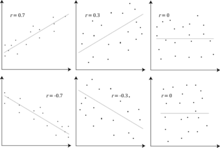
Example scatterplots of various datasets with various correlation coefficients.

The most familiar measure of dependence between two quantities is the Pearson product-moment correlation coefficient (PPMCC), or "Pearson's correlation coefficient", commonly called simply "the correlation coefficient". It is obtained by taking the ratio of the covariance of the two variables in question of our numerical dataset, normalized to the square root of their variances. Mathematically, one simply divides the covariance of the two variables by the product of their standard deviations. Karl Pearson developed the coefficient from a similar but slightly different idea by Francis Galton.

A Pearson product-moment correlation coefficient attempts to establish a line of best fit through a dataset of two variables by essentially laying out the expected values and the resulting Pearson's correlation coefficient indicates how far away the actual dataset is from the expected values. Depending on the sign of our Pearson's correlation coefficient, we can end up with either a negative or positive correlation if there is any sort of relationship between the variables of our data set.

The population correlation coefficient ${\displaystyle {\rho }_{X,Y}}$ between two random variables ${\displaystyle X}$ and ${\displaystyle Y}$ with expected values ${\displaystyle {\mu }_X}$ and ${\displaystyle {\mu }_Y}$ and standard deviations ${\displaystyle {\sigma }_X}$ and ${\displaystyle {\sigma }_Y}$ is defined as:

$${\displaystyle {\rho }_{X,Y}=\mathrm{corr}(X,Y)=\frac{\mathrm{cov}(X,Y)}{{\sigma }_X{\sigma }_Y}=\frac{\mathrm{E}[(X-{\mu }_X)(Y-{\mu }_Y)]}{{\sigma }_X{\sigma }_Y},\text{if}{\sigma }_X{\sigma }_Y>0.}$$

where ${\displaystyle \mathrm{E}}$ is the expected value operator, ${\displaystyle \mathrm{cov}}$ means covariance, and ${\displaystyle \mathrm{corr}}$ is a widely used alternative notation for the correlation coefficient. The Pearson correlation is defined only if both standard deviations are finite and positive. An alternative formula purely in terms of moments is:

$${\displaystyle {\rho }_{X,Y}=\frac{\mathrm{E}(XY)-\mathrm{E}(X)\mathrm{E}(Y)}{\sqrt{\mathrm{E}(X^2)-\mathrm{E}(X{)}^2}\cdot \sqrt{\mathrm{E}(Y^2)-\mathrm{E}(Y{)}^2}}}$$

Correlation and independence

It is a corollary of the Cauchy–Schwarz inequality that the absolute value of the Pearson correlation coefficient is not bigger than 1. Therefore, the value of a correlation coefficient ranges between −1 and +1. The correlation coefficient is +1 in the case of a perfect direct (increasing) linear relationship (correlation), −1 in the case of a perfect inverse (decreasing) linear relationship (anti-correlation), and some value in the open interval ${\displaystyle (-1,1)}$ in all other cases, indicating the degree of linear dependence between the variables. As it approaches zero there is less of a relationship (closer to uncorrelated). The closer the coefficient is to either −1 or 1, the stronger the correlation between the variables.

If the variables are independent, Pearson's correlation coefficient is 0, but the converse is not true because the correlation coefficient detects only linear dependencies between two variables.

$${\displaystyle \begin{array}{rl}X,Y\text{ independent}& \Rightarrow {\rho }_{X,Y}=0(X,Y\text{ uncorrelated})\\ {\rho }_{X,Y}=0(X,Y\text{ uncorrelated})& \nRightarrow X,Y\text{ independent}\end{array}}$$

For example, suppose the random variable ${\displaystyle X}$ is symmetrically distributed about zero, and ${\displaystyle Y=X^2}$. Then ${\displaystyle Y}$ is completely determined by ${\displaystyle X}$, so that ${\displaystyle X}$ and ${\displaystyle Y}$ are perfectly dependent, but their correlation is zero; they are uncorrelated. However, in the special case when ${\displaystyle X}$ and ${\displaystyle Y}$ are jointly normal, uncorrelatedness is equivalent to independence.

Even though uncorrelated data does not necessarily imply independence, one can check if random variables are independent if their mutual information is 0.

Sample correlation coefficient

Given a series of ${\displaystyle n}$ measurements of the pair ${\displaystyle (X_i,Y_i)}$ indexed by ${\displaystyle i=1,\dots ,n}$, the sample correlation coefficient can be used to estimate the population Pearson correlation ${\displaystyle {\rho }_{X,Y}}$ between ${\displaystyle X}$ and ${\displaystyle Y}$. The sample correlation coefficient is defined as

${\displaystyle r_{xy}\stackrel{\underset{\mathrm{d}\mathrm{e}\mathrm{f}}{}}{=}\frac{\sum _{i=1}^n(x_i-\overline{x})(y_i-\overline{y})}{(n-1)s_x{s}_y}=\frac{\sum _{i=1}^n(x_i-\overline{x})(y_i-\overline{y})}{\sqrt{\sum _{i=1}^n(x_i-\overline{x}{)}^2\sum _{i=1}^n(y_i-\overline{y}{)}^2}},}$

where ${\displaystyle \overline{x}}$ and ${\displaystyle \overline{y}}$ are the sample means of ${\displaystyle X}$ and ${\displaystyle Y}$, and ${\displaystyle s_x}$ and ${\displaystyle s_y}$ are the corrected sample standard deviations of ${\displaystyle X}$ and ${\displaystyle Y}$.

Equivalent expressions for ${\displaystyle r_{xy}}$ are

${\displaystyle \begin{array}{rl}{r}_{xy}& =\frac{\sum x_i{y}_i-n\overline{x}\overline{y}}{n{s}_x^{\prime }{s}_y^{\prime }}\\ & =\frac{n\sum x_i{y}_i-\sum x_i\sum y_i}{\sqrt{n\sum x_i^2-(\sum x_i{)}^2}\sqrt{n\sum y_i^2-(\sum y_i{)}^2}}.\end{array}}$

where ${\displaystyle s_x^{\prime }}$ and ${\displaystyle s_y^{\prime }}$ are the uncorrected sample standard deviations of ${\displaystyle X}$ and ${\displaystyle Y}$.

If ${\displaystyle x}$ and ${\displaystyle y}$ are results of measurements that contain measurement error, the realistic limits on the correlation coefficient are not −1 to +1 but a smaller range. For the case of a linear model with a single independent variable, the coefficient of determination (R squared) is the square of ${\displaystyle r_{xy}}$, Pearson's product-moment coefficient.

Example

Consider the joint probability distribution of X and Y given in the table below.

${\displaystyle \mathrm{P}(X=x,Y=y)}$

y x	−1	0	1
0	0	1/3	0
1	1/3	0	1/3

For this joint distribution, the marginal distributions are:

${\displaystyle \mathrm{P}(X=x)=\{\begin{array}{ll}\frac{1}{3}& \text{for }x=0\\ \frac{2}{3}& \text{for }x=1\end{array}}$

${\displaystyle \mathrm{P}(Y=y)=\{\begin{array}{ll}\frac{1}{3}& \text{for }y=-1\\ \frac{1}{3}& \text{for }y=0\\ \frac{1}{3}& \text{for }y=1\end{array}}$

This yields the following expectations and variances:

${\displaystyle {\mu }_X=\frac{2}{3}}$

${\displaystyle {\mu }_Y=0}$

${\displaystyle {\sigma }_X^2=\frac{2}{9}}$

${\displaystyle {\sigma }_Y^2=\frac{2}{3}}$

Therefore:

${\displaystyle \begin{array}{rl}{\rho }_{X,Y}& =\frac{1}{{\sigma }_X{\sigma }_Y}\mathrm{E}[(X-{\mu }_X)(Y-{\mu }_Y)]\\ & =\frac{1}{{\sigma }_X{\sigma }_Y}\sum _{x,y}(x-{\mu }_X)(y-{\mu }_Y)\mathrm{P}(X=x,Y=y)\\ & =\left(1-\frac{2}{3}\right)(-1-0)\frac{1}{3}+\left(0-\frac{2}{3}\right)(0-0)\frac{1}{3}+\left(1-\frac{2}{3}\right)(1-0)\frac{1}{3}=0.\end{array}}$

Rank correlation coefficients

Main articles: Spearman's rank correlation coefficient and Kendall tau rank correlation coefficient

Rank correlation coefficients, such as Spearman's rank correlation coefficient and Kendall's rank correlation coefficient (τ) measure the extent to which, as one variable increases, the other variable tends to increase, without requiring that increase to be represented by a linear relationship. If, as the one variable increases, the other decreases, the rank correlation coefficients will be negative. It is common to regard these rank correlation coefficients as alternatives to Pearson's coefficient, used either to reduce the amount of calculation or to make the coefficient less sensitive to non-normality in distributions. However, this view has little mathematical basis, as rank correlation coefficients measure a different type of relationship than the Pearson product-moment correlation coefficient, and are best seen as measures of a different type of association, rather than as an alternative measure of the population correlation coefficient.

To illustrate the nature of rank correlation, and its difference from linear correlation, consider the following four pairs of numbers ${\displaystyle (x,y)}$:

(0, 1), (10, 100), (101, 500), (102, 2000).

As we go from each pair to the next pair ${\displaystyle x}$ increases, and so does ${\displaystyle y}$. This relationship is perfect, in the sense that an increase in ${\displaystyle x}$ is always accompanied by an increase in ${\displaystyle y}$. This means that we have a perfect rank correlation, and both Spearman's and Kendall's correlation coefficients are 1, whereas in this example Pearson product-moment correlation coefficient is 0.7544, indicating that the points are far from lying on a straight line. In the same way if ${\displaystyle y}$ always decreases when ${\displaystyle x}$ increases, the rank correlation coefficients will be −1, while the Pearson product-moment correlation coefficient may or may not be close to −1, depending on how close the points are to a straight line. Although in the extreme cases of perfect rank correlation the two coefficients are both equal (being both +1 or both −1), this is not generally the case, and so values of the two coefficients cannot meaningfully be compared. For example, for the three pairs (1, 1) (2, 3) (3, 2) Spearman's coefficient is 1/2, while Kendall's coefficient is 1/3.

Other measures of dependence among random variables

See also: Pearson product-moment correlation coefficient § Variants

The information given by a correlation coefficient is not enough to define the dependence structure between random variables. The correlation coefficient completely defines the dependence structure only in very particular cases, for example when the distribution is a multivariate normal distribution. (See diagram above.) In the case of elliptical distributions it characterizes the (hyper-)ellipses of equal density; however, it does not completely characterize the dependence structure (for example, a multivariate t-distribution's degrees of freedom determine the level of tail dependence).

Distance correlation was introduced to address the deficiency of Pearson's correlation that it can be zero for dependent random variables; zero distance correlation implies independence.

The Randomized Dependence Coefficient is a computationally efficient, copula-based measure of dependence between multivariate random variables. RDC is invariant with respect to non-linear scalings of random variables, is capable of discovering a wide range of functional association patterns and takes value zero at independence.

For two binary variables, the odds ratio measures their dependence, and takes range non-negative numbers, possibly infinity: ${\displaystyle [0,+\mathrm{\infty }]}$. Related statistics such as Yule's Y and Yule's Q normalize this to the correlation-like range ${\displaystyle [-1,1]}$. The odds ratio is generalized by the logistic model to model cases where the dependent variables are discrete and there may be one or more independent variables.

The correlation ratio, entropy-based mutual information, total correlation, dual total correlation and polychoric correlation are all also capable of detecting more general dependencies, as is consideration of the copula between them, while the coefficient of determination generalizes the correlation coefficient to multiple regression.

Sensitivity to the data distribution

Further information: Pearson product-moment correlation coefficient § Sensitivity to the data distribution

The degree of dependence between variables X and Y does not depend on the scale on which the variables are expressed. That is, if we are analyzing the relationship between X and Y, most correlation measures are unaffected by transforming X to a + bX and Y to c + dY, where a, b, c, and d are constants (b and d being positive). This is true of some correlation statistics as well as their population analogues. Some correlation statistics, such as the rank correlation coefficient, are also invariant to monotone transformations of the marginal distributions of X and/or Y.

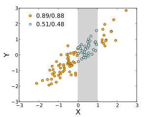
Pearson/Spearman correlation coefficients between X and Y are shown when the two variables' ranges are unrestricted, and when the range of X is restricted to the interval (0,1).

Most correlation measures are sensitive to the manner in which X and Y are sampled. Dependencies tend to be stronger if viewed over a wider range of values. Thus, if we consider the correlation coefficient between the heights of fathers and their sons over all adult males, and compare it to the same correlation coefficient calculated when the fathers are selected to be between 165 cm and 170 cm in height, the correlation will be weaker in the latter case. Several techniques have been developed that attempt to correct for range restriction in one or both variables, and are commonly used in meta-analysis; the most common are Thorndike's case II and case III equations.

Various correlation measures in use may be undefined for certain joint distributions of X and Y. For example, the Pearson correlation coefficient is defined in terms of moments, and hence will be undefined if the moments are undefined. Measures of dependence based on quantiles are always defined. Sample-based statistics intended to estimate population measures of dependence may or may not have desirable statistical properties such as being unbiased, or asymptotically consistent, based on the spatial structure of the population from which the data were sampled.

Sensitivity to the data distribution can be used to an advantage. For example, scaled correlation is designed to use the sensitivity to the range in order to pick out correlations between fast components of time series. By reducing the range of values in a controlled manner, the correlations on long time scale are filtered out and only the correlations on short time scales are revealed.

Correlation matrices

The correlation matrix of ${\displaystyle n}$ random variables ${\displaystyle X_1,\dots ,X_n}$ is the ${\displaystyle n\times n}$ matrix ${\displaystyle C}$ whose ${\displaystyle (i,j)}$ entry is

${\displaystyle c_{ij}:=\mathrm{corr}(X_i,X_j)=\frac{\mathrm{cov}(X_i,X_j)}{{\sigma }_{X_i}{\sigma }_{X_j}},\text{if}{\sigma }_{X_i}{\sigma }_{X_j}>0.}$

Thus the diagonal entries are all identically one. If the measures of correlation used are product-moment coefficients, the correlation matrix is the same as the covariance matrix of the standardized random variables ${\displaystyle X_i/\sigma (X_i)}$ for ${\displaystyle i=1,\dots ,n}$. This applies both to the matrix of population correlations (in which case ${\displaystyle \sigma }$ is the population standard deviation), and to the matrix of sample correlations (in which case ${\displaystyle \sigma }$ denotes the sample standard deviation). Consequently, each is necessarily a positive-semidefinite matrix. Moreover, the correlation matrix is strictly positive definite if no variable can have all its values exactly generated as a linear function of the values of the others.

The correlation matrix is symmetric because the correlation between ${\displaystyle X_i}$ and ${\displaystyle X_j}$ is the same as the correlation between ${\displaystyle X_j}$ and ${\displaystyle X_i}$.

A correlation matrix appears, for example, in one formula for the coefficient of multiple determination, a measure of goodness of fit in multiple regression.

In statistical modelling, correlation matrices representing the relationships between variables are categorized into different correlation structures, which are distinguished by factors such as the number of parameters required to estimate them. For example, in an exchangeable correlation matrix, all pairs of variables are modeled as having the same correlation, so all non-diagonal elements of the matrix are equal to each other. On the other hand, an autoregressive matrix is often used when variables represent a time series, since correlations are likely to be greater when measurements are closer in time. Other examples include independent, unstructured, M-dependent, and Toeplitz.

In exploratory data analysis, the iconography of correlations consists in replacing a correlation matrix by a diagram where the “remarkable” correlations are represented by a solid line (positive correlation), or a dotted line (negative correlation).

Nearest valid correlation matrix

In some applications (e.g., building data models from only partially observed data) one wants to find the "nearest" correlation matrix to an "approximate" correlation matrix (e.g., a matrix which typically lacks semi-definite positiveness due to the way it has been computed).

In 2002, Higham formalized the notion of nearness using the Frobenius norm and provided a method for computing the nearest correlation matrix using the Dykstra's projection algorithm, of which an implementation is available as an online Web API.

This sparked interest in the subject, with new theoretical (e.g., computing the nearest correlation matrix with factor structure) and numerical (e.g. usage the Newton's method for computing the nearest correlation matrix) results obtained in the subsequent years.

Uncorrelatedness and independence of stochastic processes

Similarly for two stochastic processes ${\displaystyle {\left\{X_t\right\}}_{t\in \mathcal{T}}}$ and ${\displaystyle {\left\{Y_t\right\}}_{t\in \mathcal{T}}}$: If they are independent, then they are uncorrelated. The opposite of this statement might not be true. Even if two variables are uncorrelated, they might not be independent to each other.

Common misconceptions

Correlation and causality

Main article: Correlation does not imply causation

See also: Normally distributed and uncorrelated does not imply independent

The conventional dictum that "correlation does not imply causation" means that correlation cannot be used by itself to infer a causal relationship between the variables. This dictum should not be taken to mean that correlations cannot indicate the potential existence of causal relations. However, the causes underlying the correlation, if any, may be indirect and unknown, and high correlations also overlap with identity relations (tautologies), where no causal process exists. Consequently, a correlation between two variables is not a sufficient condition to establish a causal relationship (in either direction).

A correlation between age and height in children is fairly causally transparent, but a correlation between mood and health in people is less so. Does improved mood lead to improved health, or does good health lead to good mood, or both? Or does some other factor underlie both? In other words, a correlation can be taken as evidence for a possible causal relationship, but cannot indicate what the causal relationship, if any, might be.

Simple linear correlations

Anscombe's quartet: four sets of data with the same correlation of 0.816

The Pearson correlation coefficient indicates the strength of a linear relationship between two variables, but its value generally does not completely characterize their relationship. In particular, if the conditional mean of ${\displaystyle Y}$ given ${\displaystyle X}$, denoted ${\displaystyle \mathrm{E}(Y\mid X)}$, is not linear in ${\displaystyle X}$, the correlation coefficient will not fully determine the form of ${\displaystyle \mathrm{E}(Y\mid X)}$.

The adjacent image shows scatter plots of Anscombe's quartet, a set of four different pairs of variables created by Francis Anscombe. The four ${\displaystyle y}$ variables have the same mean (7.5), variance (4.12), correlation (0.816) and regression line (y = 3 + 0.5x). However, as can be seen on the plots, the distribution of the variables is very different. The first one (top left) seems to be distributed normally, and corresponds to what one would expect when considering two variables correlated and following the assumption of normality. The second one (top right) is not distributed normally; while an obvious relationship between the two variables can be observed, it is not linear. In this case the Pearson correlation coefficient does not indicate that there is an exact functional relationship: only the extent to which that relationship can be approximated by a linear relationship. In the third case (bottom left), the linear relationship is perfect, except for one outlier which exerts enough influence to lower the correlation coefficient from 1 to 0.816. Finally, the fourth example (bottom right) shows another example when one outlier is enough to produce a high correlation coefficient, even though the relationship between the two variables is not linear.

These examples indicate that the correlation coefficient, as a summary statistic, cannot replace visual examination of the data. The examples are sometimes said to demonstrate that the Pearson correlation assumes that the data follow a normal distribution, but this is only partially correct. The Pearson correlation can be accurately calculated for any distribution that has a finite covariance matrix, which includes most distributions encountered in practice. However, the Pearson correlation coefficient (taken together with the sample mean and variance) is only a sufficient statistic if the data is drawn from a multivariate normal distribution. As a result, the Pearson correlation coefficient fully characterizes the relationship between variables if and only if the data are drawn from a multivariate normal distribution.

Bivariate normal distribution

If a pair ${\displaystyle (X,Y)}$ of random variables follows a bivariate normal distribution, the conditional mean ${\displaystyle \mathrm{E}(X\mid Y)}$ is a linear function of ${\displaystyle Y}$, and the conditional mean ${\displaystyle \mathrm{E}(Y\mid X)}$ is a linear function of ${\displaystyle X}$. The correlation coefficient ${\displaystyle {\rho }_{X,Y}}$ between ${\displaystyle X}$ and ${\displaystyle Y}$, along with the marginal means and variances of ${\displaystyle X}$ and ${\displaystyle Y}$, determines this linear relationship:

${\displaystyle \mathrm{E}(Y\mid X)=\mathrm{E}(Y)+{\rho }_{X,Y}\cdot {\sigma }_Y\frac{X-\mathrm{E}(X)}{{\sigma }_X},}$

where ${\displaystyle \mathrm{E}(X)}$ and ${\displaystyle \mathrm{E}(Y)}$ are the expected values of ${\displaystyle X}$ and ${\displaystyle Y}$, respectively, and ${\displaystyle {\sigma }_X}$ and ${\displaystyle {\sigma }_Y}$ are the standard deviations of ${\displaystyle X}$ and ${\displaystyle Y}$, respectively.

The empirical correlation ${\displaystyle r}$ is an estimate of the correlation coefficient ${\displaystyle \rho }$. A distribution estimate for ${\displaystyle \rho }$ is given by

$${\displaystyle \pi (\rho |r)=\frac{\mathrm{\Gamma }(\nu +1)}{\sqrt{2\pi }\mathrm{\Gamma }(\nu +\frac{1}{2})}(1-r^2{)}^{\frac{\nu -1}{2}}\cdot (1-{\rho }^2{)}^{\frac{\nu -2}{2}}\cdot (1-r\rho {)}^{\frac{1-2\nu }{2}}F\left(\frac{3}{2},-\frac{1}{2};\nu +\frac{1}{2};\frac{1+r\rho }{2}\right)}$$

where ${\displaystyle F}$ is the Gaussian hypergeometric function and ${\displaystyle \nu =N-1>1}$ . This density is both a Bayesian posterior density and an exact optimal confidence distribution density.