Convolutional neural network (CNN) is a regularized type of feed-forward neural network that learns feature engineering by itself via filters (or kernel) optimization. Vanishing gradients and exploding gradients, seen during backpropagation in earlier neural networks, are prevented by using regularized weights over fewer connections. For example, for each neuron in the fully-connected layer 10,000 weights would be required for processing an image sized 100 × 100 pixels. However, applying cascaded convolution (or cross-correlation) kernels, only 25 neurons are required to process 5x5-sized tiles. Higher-layer features are extracted from wider context windows, compared to lower-layer features.
They have applications in:
- image and video recognition,
- recommender systems,
- image classification,
- image segmentation,
- medical image analysis,
- natural language processing,
- brain–computer interfaces, and
- financial time series.
CNNs are also known as Shift Invariant or Space Invariant Artificial Neural Networks (SIANN), based on the shared-weight architecture of the convolution kernels or filters that slide along input features and provide translation-equivariant responses known as feature maps. Counter-intuitively, most convolutional neural networks are not invariant to translation, due to the downsampling operation they apply to the input.
Feed-forward neural networks are usually fully connected networks, that is, each neuron in one layer is connected to all neurons in the next layer. The "full connectivity" of these networks make them prone to overfitting data. Typical ways of regularization, or preventing overfitting, include: penalizing parameters during training (such as weight decay) or trimming connectivity (skipped connections, dropout, etc.) Robust datasets also increases the probability that CNNs will learn the generalized principles that characterize a given dataset rather than the biases of a poorly-populated set.
Convolutional networks were inspired by biological processes in that the connectivity pattern between neurons resembles the organization of the animal visual cortex. Individual cortical neurons respond to stimuli only in a restricted region of the visual field known as the receptive field. The receptive fields of different neurons partially overlap such that they cover the entire visual field.
CNNs use relatively little pre-processing compared to other image classification algorithms. This means that the network learns to optimize the filters (or kernels) through automated learning, whereas in traditional algorithms these filters are hand-engineered. This independence from prior knowledge and human intervention in feature extraction is a major advantage.
Architecture
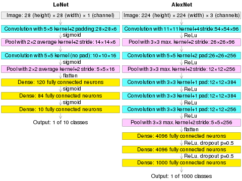
(AlexNet image size should be 227×227×3, instead of 224×224×3, so the math will come out right. The original paper said different numbers, but Andrej Karpathy, the head of computer vision at Tesla, said it should be 227×227×3 (he said Alex didn't describe why he put 224×224×3). The next convolution should be 11×11 with stride 4: 55×55×96 (instead of 54×54×96). It would be calculated, for example, as: [(input width 227 - kernel width 11) / stride 4] + 1 = [(227 - 11) / 4] + 1 = 55. Since the kernel output is the same length as width, its area is 55×55.)
A convolutional neural network consists of an input layer, hidden layers and an output layer. In a convolutional neural network, the hidden layers include one or more layers that perform convolutions. Typically this includes a layer that performs a dot product of the convolution kernel with the layer's input matrix. This product is usually the Frobenius inner product, and its activation function is commonly ReLU. As the convolution kernel slides along the input matrix for the layer, the convolution operation generates a feature map, which in turn contributes to the input of the next layer. This is followed by other layers such as pooling layers, fully connected layers, and normalization layers.
Convolutional layers
In a CNN, the input is a tensor with shape: (number of inputs) × (input height) × (input width) × (input channels). After passing through a convolutional layer, the image becomes abstracted to a feature map, also called an activation map, with shape: (number of inputs) × (feature map height) × (feature map width) × (feature map channels).
Convolutional layers convolve the input and pass its result to the next layer. This is similar to the response of a neuron in the visual cortex to a specific stimulus. Each convolutional neuron processes data only for its receptive field. Although fully connected feedforward neural networks can be used to learn features and classify data, this architecture is generally impractical for larger inputs (e.g., high-resolution images), which would require massive numbers of neurons because each pixel is a relevant input feature. A fully connected layer for an image of size 100 × 100 has 10,000 weights for each neuron in the second layer. Convolution reduces the number of free parameters, allowing the network to be deeper. For example, using a 5 × 5 tiling region, each with the same shared weights, requires only 25 neurons. Using regularized weights over fewer parameters avoids the vanishing gradients and exploding gradients problems seen during backpropagation in earlier neural networks.
To speed processing, standard convolutional layers can be replaced by depthwise separable convolutional layers, which are based on a depthwise convolution followed by a pointwise convolution. The depthwise convolution is a spatial convolution applied independently over each channel of the input tensor, while the pointwise convolution is a standard convolution restricted to the use of kernels.
Pooling layers
Convolutional networks may include local and/or global pooling layers along with traditional convolutional layers. Pooling layers reduce the dimensions of data by combining the outputs of neuron clusters at one layer into a single neuron in the next layer. Local pooling combines small clusters, tiling sizes such as 2 × 2 are commonly used. Global pooling acts on all the neurons of the feature map. There are two common types of pooling in popular use: max and average. Max pooling uses the maximum value of each local cluster of neurons in the feature map, while average pooling takes the average value.
Fully connected layers
Fully connected layers connect every neuron in one layer to every neuron in another layer. It is the same as a traditional multilayer perceptron neural network (MLP). The flattened matrix goes through a fully connected layer to classify the images.
Receptive field
In neural networks, each neuron receives input from some number of locations in the previous layer. In a convolutional layer, each neuron receives input from only a restricted area of the previous layer called the neuron's receptive field. Typically the area is a square (e.g. 5 by 5 neurons). Whereas, in a fully connected layer, the receptive field is the entire previous layer. Thus, in each convolutional layer, each neuron takes input from a larger area in the input than previous layers. This is due to applying the convolution over and over, which takes the value of a pixel into account, as well as its surrounding pixels. When using dilated layers, the number of pixels in the receptive field remains constant, but the field is more sparsely populated as its dimensions grow when combining the effect of several layers.
To manipulate the receptive field size as desired, there are some alternatives to the standard convolutional layer. For example, atrous or dilated convolution expands the receptive field size without increasing the number of parameters by interleaving visible and blind regions. Moreover, a single dilated convolutional layer can comprise filters with multiple dilation ratios, thus having a variable receptive field size.
Weights
Each neuron in a neural network computes an output value by applying a specific function to the input values received from the receptive field in the previous layer. The function that is applied to the input values is determined by a vector of weights and a bias (typically real numbers). Learning consists of iteratively adjusting these biases and weights.
The vectors of weights and biases are called filters and represent particular features of the input (e.g., a particular shape). A distinguishing feature of CNNs is that many neurons can share the same filter. This reduces the memory footprint because a single bias and a single vector of weights are used across all receptive fields that share that filter, as opposed to each receptive field having its own bias and vector weighting.
History
CNN are often compared to the way the brain achieves vision processing in living organisms.
Receptive fields in the visual cortex
Work by Hubel and Wiesel in the 1950s and 1960s showed that cat visual cortices contain neurons that individually respond to small regions of the visual field. Provided the eyes are not moving, the region of visual space within which visual stimuli affect the firing of a single neuron is known as its receptive field. Neighboring cells have similar and overlapping receptive fields. Receptive field size and location varies systematically across the cortex to form a complete map of visual space. The cortex in each hemisphere represents the contralateral visual field.
Their 1968 paper identified two basic visual cell types in the brain:
- simple cells, whose output is maximized by straight edges having particular orientations within their receptive field
- complex cells, which have larger receptive fields, whose output is insensitive to the exact position of the edges in the field.
Hubel and Wiesel also proposed a cascading model of these two types of cells for use in pattern recognition tasks.
Neocognitron, origin of the CNN architecture
The "neocognitron" was introduced by Kunihiko Fukushima in 1980. It was inspired by the above-mentioned work of Hubel and Wiesel. The neocognitron introduced the two basic types of layers in CNNs: convolutional layers, and downsampling layers. A convolutional layer contains units whose receptive fields cover a patch of the previous layer. The weight vector (the set of adaptive parameters) of such a unit is often called a filter. Units can share filters. Downsampling layers contain units whose receptive fields cover patches of previous convolutional layers. Such a unit typically computes the average of the activations of the units in its patch. This downsampling helps to correctly classify objects in visual scenes even when the objects are shifted.
In 1969, Kunihiko Fukushima also introduced the ReLU (rectified linear unit) activation function. The rectifier has become the most popular activation function for CNNs and deep neural networks in general.
In a variant of the neocognitron called the cresceptron, instead of using Fukushima's spatial averaging, J. Weng et al. in 1993 introduced a method called max-pooling where a downsampling unit computes the maximum of the activations of the units in its patch. Max-pooling is often used in modern CNNs.
Several supervised and unsupervised learning algorithms have been proposed over the decades to train the weights of a neocognitron. Today, however, the CNN architecture is usually trained through backpropagation.
The neocognitron is the first CNN which requires units located at multiple network positions to have shared weights.
Convolutional neural networks were presented at the Neural Information Processing Workshop in 1987, automatically analyzing time-varying signals by replacing learned multiplication with convolution in time, and demonstrated for speech recognition.
Time delay neural networks
The time delay neural network (TDNN) was introduced in 1987 by Alex Waibel et al. and was one of the first convolutional networks, as it achieved shift invariance. It did so by utilizing weight sharing in combination with backpropagation training. Thus, while also using a pyramidal structure as in the neocognitron, it performed a global optimization of the weights instead of a local one.
TDNNs are convolutional networks that share weights along the temporal dimension. They allow speech signals to be processed time-invariantly. In 1990 Hampshire and Waibel introduced a variant which performs a two dimensional convolution. Since these TDNNs operated on spectrograms, the resulting phoneme recognition system was invariant to both shifts in time and in frequency. This inspired translation invariance in image processing with CNNs. The tiling of neuron outputs can cover timed stages.
TDNNs now achieve the best performance in far distance speech recognition.
Max pooling
In 1990 Yamaguchi et al. introduced the concept of max pooling, which is a fixed filtering operation that calculates and propagates the maximum value of a given region. They did so by combining TDNNs with max pooling in order to realize a speaker independent isolated word recognition system. In their system they used several TDNNs per word, one for each syllable. The results of each TDNN over the input signal were combined using max pooling and the outputs of the pooling layers were then passed on to networks performing the actual word classification.
Image recognition with CNNs trained by gradient descent
A system to recognize hand-written ZIP Code numbers involved convolutions in which the kernel coefficients had been laboriously hand designed.
Yann LeCun et al. (1989) used back-propagation to learn the convolution kernel coefficients directly from images of hand-written numbers. Learning was thus fully automatic, performed better than manual coefficient design, and was suited to a broader range of image recognition problems and image types.
Wei Zhang et al. (1988) used back-propagation to train the convolution kernels of a CNN for alphabets recognition. The model was called Shift-Invariant Artificial Neural Network (SIANN) before the name CNN was coined later in the early 1990s. Wei Zhang et al. also applied the same CNN without the last fully connected layer for medical image object segmentation (1991) and breast cancer detection in mammograms (1994).
This approach became a foundation of modern computer vision.
LeNet-5
LeNet-5, a pioneering 7-level convolutional network by LeCun et al. in 1995, that classifies digits, was applied by several banks to recognize hand-written numbers on checks (British English: cheques) digitized in 32x32 pixel images. The ability to process higher-resolution images requires larger and more layers of convolutional neural networks, so this technique is constrained by the availability of computing resources.
Shift-invariant neural network
A shift-invariant neural network was proposed by Wei Zhang et al. for image character recognition in 1988. It is a modified Neocognitron by keeping only the convolutional interconnections between the image feature layers and the last fully connected layer. The model was trained with back-propagation. The training algorithm were further improved in 1991 to improve its generalization ability. The model architecture was modified by removing the last fully connected layer and applied for medical image segmentation (1991) and automatic detection of breast cancer in mammograms (1994).
A different convolution-based design was proposed in 1988 for application to decomposition of one-dimensional electromyography convolved signals via de-convolution. This design was modified in 1989 to other de-convolution-based designs.
Neural abstraction pyramid

The feed-forward architecture of convolutional neural networks was extended in the neural abstraction pyramid by lateral and feedback connections. The resulting recurrent convolutional network allows for the flexible incorporation of contextual information to iteratively resolve local ambiguities. In contrast to previous models, image-like outputs at the highest resolution were generated, e.g., for semantic segmentation, image reconstruction, and object localization tasks.
GPU implementations
Although CNNs were invented in the 1980s, their breakthrough in the 2000s required fast implementations on graphics processing units (GPUs).
In 2004, it was shown by K. S. Oh and K. Jung that standard neural networks can be greatly accelerated on GPUs. Their implementation was 20 times faster than an equivalent implementation on CPU. In 2005, another paper also emphasised the value of GPGPU for machine learning.
The first GPU-implementation of a CNN was described in 2006 by K. Chellapilla et al. Their implementation was 4 times faster than an equivalent implementation on CPU. Subsequent work also used GPUs, initially for other types of neural networks (different from CNNs), especially unsupervised neural networks.
In 2010, Dan Ciresan et al. at IDSIA showed that even deep standard neural networks with many layers can be quickly trained on GPU by supervised learning through the old method known as backpropagation. Their network outperformed previous machine learning methods on the MNIST handwritten digits benchmark. In 2011, they extended this GPU approach to CNNs, achieving an acceleration factor of 60, with impressive results. In 2011, they used such CNNs on GPU to win an image recognition contest where they achieved superhuman performance for the first time. Between May 15, 2011 and September 30, 2012, their CNNs won no less than four image competitions. In 2012, they also significantly improved on the best performance in the literature for multiple image databases, including the MNIST database, the NORB database, the HWDB1.0 dataset (Chinese characters) and the CIFAR10 dataset (dataset of 60000 32x32 labeled RGB images).
Subsequently, a similar GPU-based CNN by Alex Krizhevsky et al. won the ImageNet Large Scale Visual Recognition Challenge 2012. A very deep CNN with over 100 layers by Microsoft won the ImageNet 2015 contest.
Intel Xeon Phi implementations
Compared to the training of CNNs using GPUs, not much attention was given to the Intel Xeon Phi coprocessor. A notable development is a parallelization method for training convolutional neural networks on the Intel Xeon Phi, named Controlled Hogwild with Arbitrary Order of Synchronization (CHAOS). CHAOS exploits both the thread- and SIMD-level parallelism that is available on the Intel Xeon Phi.
Distinguishing features
In the past, traditional multilayer perceptron (MLP) models were used for image recognition. However, the full connectivity between nodes caused the curse of dimensionality, and was computationally intractable with higher-resolution images. A 1000×1000-pixel image with RGB color channels has 3 million weights per fully-connected neuron, which is too high to feasibly process efficiently at scale.

For example, in CIFAR-10, images are only of size 32×32×3 (32 wide, 32 high, 3 color channels), so a single fully connected neuron in the first hidden layer of a regular neural network would have 32*32*3 = 3,072 weights. A 200×200 image, however, would lead to neurons that have 200*200*3 = 120,000 weights.
Also, such network architecture does not take into account the spatial structure of data, treating input pixels which are far apart in the same way as pixels that are close together. This ignores locality of reference in data with a grid-topology (such as images), both computationally and semantically. Thus, full connectivity of neurons is wasteful for purposes such as image recognition that are dominated by spatially local input patterns.
Convolutional neural networks are variants of multilayer perceptrons, designed to emulate the behavior of a visual cortex. These models mitigate the challenges posed by the MLP architecture by exploiting the strong spatially local correlation present in natural images. As opposed to MLPs, CNNs have the following distinguishing features:
- 3D volumes of neurons. The layers of a CNN have neurons arranged in 3 dimensions: width, height and depth. Where each neuron inside a convolutional layer is connected to only a small region of the layer before it, called a receptive field. Distinct types of layers, both locally and completely connected, are stacked to form a CNN architecture.
- Local connectivity: following the concept of receptive fields, CNNs exploit spatial locality by enforcing a local connectivity pattern between neurons of adjacent layers. The architecture thus ensures that the learned "filters" produce the strongest response to a spatially local input pattern. Stacking many such layers leads to nonlinear filters that become increasingly global (i.e. responsive to a larger region of pixel space) so that the network first creates representations of small parts of the input, then from them assembles representations of larger areas.
- Shared weights: In CNNs, each filter is replicated across the entire visual field. These replicated units share the same parameterization (weight vector and bias) and form a feature map. This means that all the neurons in a given convolutional layer respond to the same feature within their specific response field. Replicating units in this way allows for the resulting activation map to be equivariant under shifts of the locations of input features in the visual field, i.e. they grant translational equivariance - given that the layer has a stride of one.
- Pooling: In a CNN's pooling layers, feature maps are divided into rectangular sub-regions, and the features in each rectangle are independently down-sampled to a single value, commonly by taking their average or maximum value. In addition to reducing the sizes of feature maps, the pooling operation grants a degree of local translational invariance to the features contained therein, allowing the CNN to be more robust to variations in their positions.
Together, these properties allow CNNs to achieve better generalization on vision problems. Weight sharing dramatically reduces the number of free parameters learned, thus lowering the memory requirements for running the network and allowing the training of larger, more powerful networks.
Building blocks
A CNN architecture is formed by a stack of distinct layers that transform the input volume into an output volume (e.g. holding the class scores) through a differentiable function. A few distinct types of layers are commonly used. These are further discussed below.

Convolutional layer
The convolutional layer is the core building block of a CNN. The layer's parameters consist of a set of learnable filters (or kernels), which have a small receptive field, but extend through the full depth of the input volume. During the forward pass, each filter is convolved across the width and height of the input volume, computing the dot product between the filter entries and the input, producing a 2-dimensional activation map of that filter. As a result, the network learns filters that activate when it detects some specific type of feature at some spatial position in the input.
Stacking the activation maps for all filters along the depth dimension forms the full output volume of the convolution layer. Every entry in the output volume can thus also be interpreted as an output of a neuron that looks at a small region in the input and shares parameters with neurons in the same activation map.
Self-supervised learning has been adapted for use in convolutional layers by using sparse patches with a high-mask ratio and a global response normalization layer.
Local connectivity

When dealing with high-dimensional inputs such as images, it is impractical to connect neurons to all neurons in the previous volume because such a network architecture does not take the spatial structure of the data into account. Convolutional networks exploit spatially local correlation by enforcing a sparse local connectivity pattern between neurons of adjacent layers: each neuron is connected to only a small region of the input volume.
The extent of this connectivity is a hyperparameter called the receptive field of the neuron. The connections are local in space (along width and height), but always extend along the entire depth of the input volume. Such an architecture ensures that the learned (British English: learnt) filters produce the strongest response to a spatially local input pattern.
Spatial arrangement
Three hyperparameters control the size of the output volume of the convolutional layer: the depth, stride, and padding size:
- The depth of the output volume controls the number of neurons in a layer that connect to the same region of the input volume. These neurons learn to activate for different features in the input. For example, if the first convolutional layer takes the raw image as input, then different neurons along the depth dimension may activate in the presence of various oriented edges, or blobs of color.
- Stride controls how depth columns around the width and height are allocated. If the stride is 1, then we move the filters one pixel at a time. This leads to heavily overlapping receptive fields between the columns, and to large output volumes. For any integer a stride S means that the filter is translated S units at a time per output. In practice, is rare. A greater stride means smaller overlap of receptive fields and smaller spatial dimensions of the output volume.
- Sometimes, it is convenient to pad the input with zeros (or other values, such as the average of the region) on the border of the input volume. The size of this padding is a third hyperparameter. Padding provides control of the output volume's spatial size. In particular, sometimes it is desirable to exactly preserve the spatial size of the input volume, this is commonly referred to as "same" padding.
The spatial size of the output volume is a function of the input volume size , the kernel field size of the convolutional layer neurons, the stride , and the amount of zero padding on the border. The number of neurons that "fit" in a given volume is then:
If this number is not an integer, then the strides are incorrect and the neurons cannot be tiled to fit across the input volume in a symmetric way. In general, setting zero padding to be when the stride is ensures that the input volume and output volume will have the same size spatially. However, it is not always completely necessary to use all of the neurons of the previous layer. For example, a neural network designer may decide to use just a portion of padding.
Parameter sharing
A parameter sharing scheme is used in convolutional layers to control the number of free parameters. It relies on the assumption that if a patch feature is useful to compute at some spatial position, then it should also be useful to compute at other positions. Denoting a single 2-dimensional slice of depth as a depth slice, the neurons in each depth slice are constrained to use the same weights and bias.
Since all neurons in a single depth slice share the same parameters, the forward pass in each depth slice of the convolutional layer can be computed as a convolution of the neuron's weights with the input volume. Therefore, it is common to refer to the sets of weights as a filter (or a kernel), which is convolved with the input. The result of this convolution is an activation map, and the set of activation maps for each different filter are stacked together along the depth dimension to produce the output volume. Parameter sharing contributes to the translation invariance of the CNN architecture.
Sometimes, the parameter sharing assumption may not make sense. This is especially the case when the input images to a CNN have some specific centered structure; for which we expect completely different features to be learned on different spatial locations. One practical example is when the inputs are faces that have been centered in the image: we might expect different eye-specific or hair-specific features to be learned in different parts of the image. In that case it is common to relax the parameter sharing scheme, and instead simply call the layer a "locally connected layer".
Pooling layer

Another important concept of CNNs is pooling, which is a form of non-linear down-sampling. There are several non-linear functions to implement pooling, where max pooling is the most common. It partitions the input image into a set of rectangles and, for each such sub-region, outputs the maximum.
Intuitively, the exact location of a feature is less important than its rough location relative to other features. This is the idea behind the use of pooling in convolutional neural networks. The pooling layer serves to progressively reduce the spatial size of the representation, to reduce the number of parameters, memory footprint and amount of computation in the network, and hence to also control overfitting. This is known as down-sampling. It is common to periodically insert a pooling layer between successive convolutional layers (each one typically followed by an activation function, such as a ReLU layer) in a CNN architecture. While pooling layers contribute to local translation invariance, they do not provide global translation invariance in a CNN, unless a form of global pooling is used. The pooling layer commonly operates independently on every depth, or slice, of the input and resizes it spatially. A very common form of max pooling is a layer with filters of size 2×2, applied with a stride of 2, which subsamples every depth slice in the input by 2 along both width and height, discarding 75% of the activations:
In addition to max pooling, pooling units can use other functions, such as average pooling or ℓ2-norm pooling. Average pooling was often used historically but has recently fallen out of favor compared to max pooling, which generally performs better in practice.
Due to the effects of fast spatial reduction of the size of the representation, there is a recent trend towards using smaller filters or discarding pooling layers altogether.

"Region of Interest" pooling (also known as RoI pooling) is a variant of max pooling, in which output size is fixed and input rectangle is a parameter.
Pooling is a downsampling method and an important component of convolutional neural networks for object detection based on the Fast R-CNN architecture.
Channel Max Pooling
A CMP operation layer conducts the MP operation along the channel side among the corresponding positions of the consecutive feature maps for the purpose of redundant information elimination. The CMP makes the significant features gather together within fewer channels, which is important for fine-grained image classification that needs more discriminating features. Meanwhile, another advantage of the CMP operation is to make the channel number of feature maps smaller before it connects to the first fully connected (FC) layer. Similar to the MP operation, we denote the input feature maps and output feature maps of a CMP layer as F ∈ R(C×M×N) and C ∈ R(c×M×N), respectively, where C and c are the channel numbers of the input and output feature maps, M and N are the widths and the height of the feature maps, respectively. Note that the CMP operation only changes the channel number of the feature maps. The width and the height of the feature maps are not changed, which is different from the MP operation.
ReLU layer
ReLU is the abbreviation of rectified linear unit introduced by Kunihiko Fukushima in 1969. ReLU applies the non-saturating activation function . It effectively removes negative values from an activation map by setting them to zero. It introduces nonlinearity to the decision function and in the overall network without affecting the receptive fields of the convolution layers. In 2011, Xavier Glorot, Antoine Bordes and Yoshua Bengio found that ReLU enables better training of deeper networks, compared to widely used activation functions prior to 2011.
Other functions can also be used to increase nonlinearity, for example the saturating hyperbolic tangent , , and the sigmoid function . ReLU is often preferred to other functions because it trains the neural network several times faster without a significant penalty to generalization accuracy.
Fully connected layer
After several convolutional and max pooling layers, the final classification is done via fully connected layers. Neurons in a fully connected layer have connections to all activations in the previous layer, as seen in regular (non-convolutional) artificial neural networks. Their activations can thus be computed as an affine transformation, with matrix multiplication followed by a bias offset (vector addition of a learned or fixed bias term).
Loss layer
The "loss layer", or "loss function", specifies how training penalizes the deviation between the predicted output of the network, and the true data labels (during supervised learning). Various loss functions can be used, depending on the specific task.
The Softmax loss function is used for predicting a single class of K mutually exclusive classes. Sigmoid cross-entropy loss is used for predicting K independent probability values in . Euclidean loss is used for regressing to real-valued labels .
Hyperparameters
Hyperparameters are various settings that are used to control the learning process. CNNs use more hyperparameters than a standard multilayer perceptron (MLP).
Kernel size
The kernel is the number of pixels processed together. It is typically expressed as the kernel's dimensions, e.g., 2x2, or 3x3.
Padding
Padding is the addition of (typically) 0-valued pixels on the borders of an image. This is done so that the border pixels are not undervalued (lost) from the output because they would ordinarily participate in only a single receptive field instance. The padding applied is typically one less than the corresponding kernel dimension. For example, a convolutional layer using 3x3 kernels would receive a 2-pixel pad, that is 1 pixel on each side of the image.
Stride
The stride is the number of pixels that the analysis window moves on each iteration. A stride of 2 means that each kernel is offset by 2 pixels from its predecessor.
Number of filters
Since feature map size decreases with depth, layers near the input layer tend to have fewer filters while higher layers can have more. To equalize computation at each layer, the product of feature values va with pixel position is kept roughly constant across layers. Preserving more information about the input would require keeping the total number of activations (number of feature maps times number of pixel positions) non-decreasing from one layer to the next.
The number of feature maps directly controls the capacity and depends on the number of available examples and task complexity.
Filter size
Common filter sizes found in the literature vary greatly, and are usually chosen based on the data set.
The challenge is to find the right level of granularity so as to create abstractions at the proper scale, given a particular data set, and without overfitting.
Pooling type and size
Max pooling is typically used, often with a 2x2 dimension. This implies that the input is drastically downsampled, reducing processing cost.
Large input volumes may warrant 4×4 pooling in the lower layers. Greater pooling reduces the dimension of the signal, and may result in unacceptable information loss. Often, non-overlapping pooling windows perform best.
Dilation
Dilation involves ignoring pixels within a kernel. This reduces processing/memory potentially without significant signal loss. A dilation of 2 on a 3x3 kernel expands the kernel to 5x5, while still processing 9 (evenly spaced) pixels. Accordingly, dilation of 4 expands the kernel to 9x9.
Translation equivariance and aliasing
It is commonly assumed that CNNs are invariant to shifts of the input. Convolution or pooling layers within a CNN that do not have a stride greater than one are indeed equivariant to translations of the input. However, layers with a stride greater than one ignore the Nyquist-Shannon sampling theorem and might lead to aliasing of the input signal While, in principle, CNNs are capable of implementing anti-aliasing filters, it has been observed that this does not happen in practice and yield models that are not equivariant to translations. Furthermore, if a CNN makes use of fully connected layers, translation equivariance does not imply translation invariance, as the fully connected layers are not invariant to shifts of the input. One solution for complete translation invariance is avoiding any down-sampling throughout the network and applying global average pooling at the last layer. Additionally, several other partial solutions have been proposed, such as anti-aliasing before downsampling operations, spatial transformer networks, data augmentation, subsampling combined with pooling, and capsule neural networks.
Evaluation
The accuracy of the final model is based on a sub-part of the dataset set apart at the start, often called a test-set. Other times methods such as k-fold cross-validation are applied. Other strategies include using conformal prediction.
Regularization methods
Regularization is a process of introducing additional information to solve an ill-posed problem or to prevent overfitting. CNNs use various types of regularization.
Empirical
Dropout
Because a fully connected layer occupies most of the parameters, it is prone to overfitting. One method to reduce overfitting is dropout, introduced in 2014. At each training stage, individual nodes are either "dropped out" of the net (ignored) with probability or kept with probability , so that a reduced network is left; incoming and outgoing edges to a dropped-out node are also removed. Only the reduced network is trained on the data in that stage. The removed nodes are then reinserted into the network with their original weights.
In the training stages, is usually 0.5; for input nodes, it is typically much higher because information is directly lost when input nodes are ignored.
At testing time after training has finished, we would ideally like to find a sample average of all possible dropped-out networks; unfortunately this is unfeasible for large values of . However, we can find an approximation by using the full network with each node's output weighted by a factor of , so the expected value of the output of any node is the same as in the training stages. This is the biggest contribution of the dropout method: although it effectively generates neural nets, and as such allows for model combination, at test time only a single network needs to be tested.
By avoiding training all nodes on all training data, dropout decreases overfitting. The method also significantly improves training speed. This makes the model combination practical, even for deep neural networks. The technique seems to reduce node interactions, leading them to learn more robust features that better generalize to new data.
DropConnect
DropConnect is the generalization of dropout in which each connection, rather than each output unit, can be dropped with probability . Each unit thus receives input from a random subset of units in the previous layer.
DropConnect is similar to dropout as it introduces dynamic sparsity within the model, but differs in that the sparsity is on the weights, rather than the output vectors of a layer. In other words, the fully connected layer with DropConnect becomes a sparsely connected layer in which the connections are chosen at random during the training stage.
Stochastic pooling
A major drawback to Dropout is that it does not have the same benefits for convolutional layers, where the neurons are not fully connected.
Even before Dropout, in 2013 a technique called stochastic pooling, the conventional deterministic pooling operations were replaced with a stochastic procedure, where the activation within each pooling region is picked randomly according to a multinomial distribution, given by the activities within the pooling region. This approach is free of hyperparameters and can be combined with other regularization approaches, such as dropout and data augmentation.
An alternate view of stochastic pooling is that it is equivalent to standard max pooling but with many copies of an input image, each having small local deformations. This is similar to explicit elastic deformations of the input images, which delivers excellent performance on the MNIST data set. Using stochastic pooling in a multilayer model gives an exponential number of deformations since the selections in higher layers are independent of those below.
Artificial data
Because the degree of model overfitting is determined by both its power and the amount of training it receives, providing a convolutional network with more training examples can reduce overfitting. Because there is often not enough available data to train, especially considering that some part should be spared for later testing, two approaches are to either generate new data from scratch (if possible) or perturb existing data to create new ones. The latter one is used since mid-1990s. For example, input images can be cropped, rotated, or rescaled to create new examples with the same labels as the original training set.
Explicit
Early stopping
One of the simplest methods to prevent overfitting of a network is to simply stop the training before overfitting has had a chance to occur. It comes with the disadvantage that the learning process is halted.
Number of parameters
Another simple way to prevent overfitting is to limit the number of parameters, typically by limiting the number of hidden units in each layer or limiting network depth. For convolutional networks, the filter size also affects the number of parameters. Limiting the number of parameters restricts the predictive power of the network directly, reducing the complexity of the function that it can perform on the data, and thus limits the amount of overfitting. This is equivalent to a "zero norm".
Weight decay
A simple form of added regularizer is weight decay, which simply adds an additional error, proportional to the sum of weights (L1 norm) or squared magnitude (L2 norm) of the weight vector, to the error at each node. The level of acceptable model complexity can be reduced by increasing the proportionality constant('alpha' hyperparameter), thus increasing the penalty for large weight vectors.
L2 regularization is the most common form of regularization. It can be implemented by penalizing the squared magnitude of all parameters directly in the objective. The L2 regularization has the intuitive interpretation of heavily penalizing peaky weight vectors and preferring diffuse weight vectors. Due to multiplicative interactions between weights and inputs this has the useful property of encouraging the network to use all of its inputs a little rather than some of its inputs a lot.
L1 regularization is also common. It makes the weight vectors sparse during optimization. In other words, neurons with L1 regularization end up using only a sparse subset of their most important inputs and become nearly invariant to the noisy inputs. L1 with L2 regularization can be combined; this is called elastic net regularization.
Max norm constraints
Another form of regularization is to enforce an absolute upper bound on the magnitude of the weight vector for every neuron and use projected gradient descent to enforce the constraint. In practice, this corresponds to performing the parameter update as normal, and then enforcing the constraint by clamping the weight vector of every neuron to satisfy . Typical values of are order of 3–4. Some papers report improvements when using this form of regularization.
Hierarchical coordinate frames
Pooling loses the precise spatial relationships between high-level parts (such as nose and mouth in a face image). These relationships are needed for identity recognition. Overlapping the pools so that each feature occurs in multiple pools, helps retain the information. Translation alone cannot extrapolate the understanding of geometric relationships to a radically new viewpoint, such as a different orientation or scale. On the other hand, people are very good at extrapolating; after seeing a new shape once they can recognize it from a different viewpoint.
An earlier common way to deal with this problem is to train the network on transformed data in different orientations, scales, lighting, etc. so that the network can cope with these variations. This is computationally intensive for large data-sets. The alternative is to use a hierarchy of coordinate frames and use a group of neurons to represent a conjunction of the shape of the feature and its pose relative to the retina. The pose relative to the retina is the relationship between the coordinate frame of the retina and the intrinsic features' coordinate frame.
Thus, one way to represent something is to embed the coordinate frame within it. This allows large features to be recognized by using the consistency of the poses of their parts (e.g. nose and mouth poses make a consistent prediction of the pose of the whole face). This approach ensures that the higher-level entity (e.g. face) is present when the lower-level (e.g. nose and mouth) agree on its prediction of the pose. The vectors of neuronal activity that represent pose ("pose vectors") allow spatial transformations modeled as linear operations that make it easier for the network to learn the hierarchy of visual entities and generalize across viewpoints. This is similar to the way the human visual system imposes coordinate frames in order to represent shapes.
Applications
Image recognition
CNNs are often used in image recognition systems. In 2012, an error rate of 0.23% on the MNIST database was reported. Another paper on using CNN for image classification reported that the learning process was "surprisingly fast"; in the same paper, the best published results as of 2011 were achieved in the MNIST database and the NORB database. Subsequently, a similar CNN called AlexNet won the ImageNet Large Scale Visual Recognition Challenge 2012.
When applied to facial recognition, CNNs achieved a large decrease in error rate. Another paper reported a 97.6% recognition rate on "5,600 still images of more than 10 subjects". CNNs were used to assess video quality in an objective way after manual training; the resulting system had a very low root mean square error.
The ImageNet Large Scale Visual Recognition Challenge is a benchmark in object classification and detection, with millions of images and hundreds of object classes. In the ILSVRC 2014, a large-scale visual recognition challenge, almost every highly ranked team used CNN as their basic framework. The winner GoogLeNet (the foundation of DeepDream) increased the mean average precision of object detection to 0.439329, and reduced classification error to 0.06656, the best result to date. Its network applied more than 30 layers. That performance of convolutional neural networks on the ImageNet tests was close to that of humans. The best algorithms still struggle with objects that are small or thin, such as a small ant on a stem of a flower or a person holding a quill in their hand. They also have trouble with images that have been distorted with filters, an increasingly common phenomenon with modern digital cameras. By contrast, those kinds of images rarely trouble humans. Humans, however, tend to have trouble with other issues. For example, they are not good at classifying objects into fine-grained categories such as the particular breed of dog or species of bird, whereas convolutional neural networks handle this.
In 2015, a many-layered CNN demonstrated the ability to spot faces from a wide range of angles, including upside down, even when partially occluded, with competitive performance. The network was trained on a database of 200,000 images that included faces at various angles and orientations and a further 20 million images without faces. They used batches of 128 images over 50,000 iterations.
Video analysis
Compared to image data domains, there is relatively little work on applying CNNs to video classification. Video is more complex than images since it has another (temporal) dimension. However, some extensions of CNNs into the video domain have been explored. One approach is to treat space and time as equivalent dimensions of the input and perform convolutions in both time and space. Another way is to fuse the features of two convolutional neural networks, one for the spatial and one for the temporal stream. Long short-term memory (LSTM) recurrent units are typically incorporated after the CNN to account for inter-frame or inter-clip dependencies. Unsupervised learning schemes for training spatio-temporal features have been introduced, based on Convolutional Gated Restricted Boltzmann Machines and Independent Subspace Analysis. It's Application can be seen in Text-to-Video model.
Natural language processing
CNNs have also been explored for natural language processing. CNN models are effective for various NLP problems and achieved excellent results in semantic parsing, search query retrieval, sentence modeling, classification, prediction and other traditional NLP tasks. Compared to traditional language processing methods such as recurrent neural networks, CNNs can represent different contextual realities of language that do not rely on a series-sequence assumption, while RNNs are better suitable when classical time series modeling is required.
Anomaly Detection
A CNN with 1-D convolutions was used on time series in the frequency domain (spectral residual) by an unsupervised model to detect anomalies in the time domain.
Drug discovery
CNNs have been used in drug discovery. Predicting the interaction between molecules and biological proteins can identify potential treatments. In 2015, Atomwise introduced AtomNet, the first deep learning neural network for structure-based drug design. The system trains directly on 3-dimensional representations of chemical interactions. Similar to how image recognition networks learn to compose smaller, spatially proximate features into larger, complex structures, AtomNet discovers chemical features, such as aromaticity, sp3 carbons, and hydrogen bonding. Subsequently, AtomNet was used to predict novel candidate biomolecules for multiple disease targets, most notably treatments for the Ebola virus and multiple sclerosis.
Checkers game
CNNs have been used in the game of checkers. From 1999 to 2001, Fogel and Chellapilla published papers showing how a convolutional neural network could learn to play checker using co-evolution. The learning process did not use prior human professional games, but rather focused on a minimal set of information contained in the checkerboard: the location and type of pieces, and the difference in number of pieces between the two sides. Ultimately, the program (Blondie24) was tested on 165 games against players and ranked in the highest 0.4%. It also earned a win against the program Chinook at its "expert" level of play.
Go
CNNs have been used in computer Go. In December 2014, Clark and Storkey published a paper showing that a CNN trained by supervised learning from a database of human professional games could outperform GNU Go and win some games against Monte Carlo tree search Fuego 1.1 in a fraction of the time it took Fuego to play. Later it was announced that a large 12-layer convolutional neural network had correctly predicted the professional move in 55% of positions, equalling the accuracy of a 6 dan human player. When the trained convolutional network was used directly to play games of Go, without any search, it beat the traditional search program GNU Go in 97% of games, and matched the performance of the Monte Carlo tree search program Fuego simulating ten thousand playouts (about a million positions) per move.
A couple of CNNs for choosing moves to try ("policy network") and evaluating positions ("value network") driving MCTS were used by AlphaGo, the first to beat the best human player at the time.
Time series forecasting
Recurrent neural networks are generally considered the best neural network architectures for time series forecasting (and sequence modeling in general), but recent studies show that convolutional networks can perform comparably or even better. Dilated convolutions might enable one-dimensional convolutional neural networks to effectively learn time series dependences. Convolutions can be implemented more efficiently than RNN-based solutions, and they do not suffer from vanishing (or exploding) gradients. Convolutional networks can provide an improved forecasting performance when there are multiple similar time series to learn from. CNNs can also be applied to further tasks in time series analysis (e.g., time series classification or quantile forecasting).
Cultural Heritage and 3D-datasets
As archaeological findings like clay tablets with cuneiform writing are increasingly acquired using 3D scanners first benchmark datasets are becoming available like HeiCuBeDa providing almost 2.000 normalized 2D- and 3D-datasets prepared with the GigaMesh Software Framework. So curvature-based measures are used in conjunction with Geometric Neural Networks (GNNs) e.g. for period classification of those clay tablets being among the oldest documents of human history.
Fine-tuning
For many applications, the training data is less available. Convolutional neural networks usually require a large amount of training data in order to avoid overfitting. A common technique is to train the network on a larger data set from a related domain. Once the network parameters have converged an additional training step is performed using the in-domain data to fine-tune the network weights, this is known as transfer learning. Furthermore, this technique allows convolutional network architectures to successfully be applied to problems with tiny training sets.
Human interpretable explanations
End-to-end training and prediction are common practice in computer vision. However, human interpretable explanations are required for critical systems such as a self-driving cars. With recent advances in visual salience, spatial attention, and temporal attention, the most critical spatial regions/temporal instants could be visualized to justify the CNN predictions.
Related architectures
Deep Q-networks
A deep Q-network (DQN) is a type of deep learning model that combines a deep neural network with Q-learning, a form of reinforcement learning. Unlike earlier reinforcement learning agents, DQNs that utilize CNNs can learn directly from high-dimensional sensory inputs via reinforcement learning.
Preliminary results were presented in 2014, with an accompanying paper in February 2015. The research described an application to Atari 2600 gaming. Other deep reinforcement learning models preceded it.
Deep belief networks
Convolutional deep belief networks (CDBN) have structure very similar to convolutional neural networks and are trained similarly to deep belief networks. Therefore, they exploit the 2D structure of images, like CNNs do, and make use of pre-training like deep belief networks. They provide a generic structure that can be used in many image and signal processing tasks. Benchmark results on standard image datasets like CIFAR have been obtained using CDBNs.
Notable libraries
- Caffe: A library for convolutional neural networks. Created by the Berkeley Vision and Learning Center (BVLC). It supports both CPU and GPU. Developed in C++, and has Python and MATLAB wrappers.
- Deeplearning4j: Deep learning in Java and Scala on multi-GPU-enabled Spark. A general-purpose deep learning library for the JVM production stack running on a C++ scientific computing engine. Allows the creation of custom layers. Integrates with Hadoop and Kafka.
- Dlib: A toolkit for making real world machine learning and data analysis applications in C++.
- Microsoft Cognitive Toolkit: A deep learning toolkit written by Microsoft with several unique features enhancing scalability over multiple nodes. It supports full-fledged interfaces for training in C++ and Python and with additional support for model inference in C# and Java.
- TensorFlow: Apache 2.0-licensed Theano-like library with support for CPU, GPU, Google's proprietary tensor processing unit (TPU), and mobile devices.
- Theano: The reference deep-learning library for Python with an API largely compatible with the popular NumPy library. Allows user to write symbolic mathematical expressions, then automatically generates their derivatives, saving the user from having to code gradients or backpropagation. These symbolic expressions are automatically compiled to CUDA code for a fast, on-the-GPU implementation.
- Torch: A scientific computing framework with wide support for machine learning algorithms, written in C and Lua.


![[0,1]](https://wikimedia.org/api/rest_v1/media/math/render/svg/738f7d23bb2d9642bab520020873cccbef49768d)


