Van Allen radiation belt

From Wikipedia, the free encyclopedia

 

A cross section of Van Allen radiation belts

 

A Van Allen radiation belt is a zone of energetic charged particles, most of which originate from the solar wind, that are captured by and held around a planet by that planet's magnetic field. Earth has two such belts and sometimes others may be temporarily created. The discovery of the belts is credited to James Van Allen, and as a result, Earth's belts are known as the Van Allen belts. Earth's two main belts extend from an altitude of about 640 to 58,000 km (400 to 36,040 mi) above the surface in which region radiation levels vary. Most of the particles that form the belts are thought to come from solar wind and other particles by cosmic rays. By trapping the solar wind, the magnetic field deflects those energetic particles and protects the atmosphere from destruction.

The belts are located in the inner region of Earth's magnetosphere. The belts trap energetic electrons and protons. Other nuclei, such as alpha particles, are less prevalent. The belts endanger satellites, which must have their sensitive components protected with adequate shielding if they spend significant time near that zone. In 2013, NASA reported that the Van Allen Probes had discovered a transient, third radiation belt, which was observed for four weeks until it was destroyed by a powerful, interplanetary shock wave from the Sun.

Discovery

Kristian Birkeland, Carl Størmer, and Nicholas Christofilos had investigated the possibility of trapped charged particles before the Space Age. Explorer 1 and Explorer 3 confirmed the existence of the belt in early 1958 under James Van Allen at the University of Iowa. The trapped radiation was first mapped by Explorer 4, Pioneer 3 and Luna 1. 

The term Van Allen belts refers specifically to the radiation belts surrounding Earth; however, similar radiation belts have been discovered around other planets. The Sun does not support long-term radiation belts, as it lacks a stable, global, dipole field. The Earth's atmosphere limits the belts' particles to regions above 200–1,000 km, (124–620 miles) while the belts do not extend past 8 Earth radii R_E. The belts are confined to a volume which extends about 65° on either side of the celestial equator.

Research

Jupiter's variable radiation belts

 

The NASA Van Allen Probes mission aims at understanding (to the point of predictability) how populations of relativistic electrons and ions in space form or change in response to changes in solar activity and the solar wind. NASA Institute for Advanced Concepts–funded studies have proposed magnetic scoops to collect antimatter that naturally occurs in the Van Allen belts of Earth, although only about 10 micrograms of antiprotons are estimated to exist in the entire belt.

The Van Allen Probes mission successfully launched on August 30, 2012. The primary mission is scheduled to last two years with expendables expected to last four. NASA's Goddard Space Flight Center manages the Living With a Star program of which the Van Allen Probes is a project, along with Solar Dynamics Observatory (SDO). The Applied Physics Laboratory is responsible for the implementation and instrument management for the Van Allen Probes.

Radiation belts exist around other planets and moons in the solar system that have magnetic fields powerful enough to sustain them. To date, most of these radiation belts have been poorly mapped. The Voyager Program (namely Voyager 2) only nominally confirmed the existence of similar belts around Uranus and Neptune.

Inner belt

Cutaway drawing of two radiation belts around Earth: the inner belt (red) dominated by protons and the outer one (blue) by electrons. Image Credit: NASA

 

The inner Van Allen Belt extends typically from an altitude of 0.2 to 2 Earth radii (L values of 1 to 3) or 1,000 km (620 mi) to 6,000 km (3,700 mi) above the Earth. In certain cases when solar activity is stronger or in geographical areas such as the South Atlantic Anomaly, the inner boundary may decline to roughly 200 kilometers above the Earth's surface. The inner belt contains high concentrations of electrons in the range of hundreds of keV and energetic protons with energies exceeding 100 MeV, trapped by the strong (relative to the outer belts) magnetic fields in the region.

It is believed that proton energies exceeding 50 MeV in the lower belts at lower altitudes are the result of the beta decay of neutrons created by cosmic ray collisions with nuclei of the upper atmosphere. The source of lower energy protons is believed to be proton diffusion due to changes in the magnetic field during geomagnetic storms.

Due to the slight offset of the belts from Earth's geometric center, the inner Van Allen belt makes its closest approach to the surface at the South Atlantic Anomaly.

On March 2014, a pattern resembling 'zebra stripes' was observed in the radiation belts by the Radiation Belt Storm Probes Ion Composition Experiment (RBSPICE) onboard Van Allen Probes. The reason reported was that due to the tilt in Earth's magnetic field axis, the planet's rotation generated an oscillating, weak electric field that permeates through the entire inner radiation belt. It was later demonstrated that the zebra stripes were in fact an imprint of ionospheric winds on radiation belts.

Outer belt

Laboratory simulation of the Van Allen belt's influence on the Solar Wind; these aurora-like Birkeland currents were created by the scientist Kristian Birkeland in his terrella, a magnetized anode globe in an evacuated chamber

 

The outer belt consists mainly of high energy (0.1–10 MeV) electrons trapped by the Earth's magnetosphere. It is more variable than the inner belt as it is more easily influenced by solar activity. It is almost toroidal in shape, beginning at an altitude of three and extending to ten Earth radii (R_E) 13,000 to 60,000 kilometres (8,100 to 37,300 mi) above the Earth's surface. Its greatest intensity is usually around 4–5 R_E. The outer electron radiation belt is mostly produced by the inward radial diffusion and local acceleration due to transfer of energy from whistler-mode plasma waves to radiation belt electrons. Radiation belt electrons are also constantly removed by collisions with Earth's atmosphere, losses to the magnetopause, and their outward radial diffusion. The gyroradii of energetic protons would be large enough to bring them into contact with the Earth's atmosphere. Within this belt, the electrons have a high flux and at the outer edge (close to the magnetopause), where geomagnetic field lines open into the geomagnetic "tail", the flux of energetic electrons can drop to the low interplanetary levels within about 100 km (62 mi), a decrease by a factor of 1,000.

In 2014 it was discovered that the inner edge of the outer belt is characterized by a very sharp transition, below which highly relativistic electrons (> 5MeV) cannot penetrate. The reason for this shield-like behavior is not well understood. 

The trapped particle population of the outer belt is varied, containing electrons and various ions. Most of the ions are in the form of energetic protons, but a certain percentage are alpha particles and O⁺ oxygen ions, similar to those in the ionosphere but are much more energetic. This mixture of ions suggests that ring current particles probably come from more than one source.

The outer belt is larger than the inner belt and its particle population fluctuates widely. Energetic (radiation) particle fluxes can increase and decrease dramatically in response to geomagnetic storms, which are themselves triggered by magnetic field and plasma disturbances produced by the Sun. The increases are due to storm-related injections and acceleration of particles from the tail of the magnetosphere.

On February 28, 2013, a third radiation belt, consisting of high-energy ultrarelativistic charged particles, was reported to be discovered. In a news conference by NASA's Van Allen Probe team, it was stated that this third belt is a product of coronal mass ejection from the Sun. It has been represented as a separate creation which splits the Outer Belt, like a knife, on its outer side, and exists separately as a storage container of particles for a month's time, before merging once again with the Outer Belt.

The unusual stability of this third, transient belt has been explained as due to a 'trapping' by the Earth's magnetic field of ultrarelativistic particles as they are lost from the second, traditional outer belt. While the outer zone, which forms and disappears over a day, is highly variable due to interactions with the atmosphere, the ultrarelativistic particles of the third belt are thought to not scatter into the atmosphere, as they are too energetic to interact with atmospheric waves at low latitudes. This absence of scattering and the trapping allows them to persist for a long time, finally only being destroyed by an unusual event, such as the shock wave from the Sun.

Flux values

In the belts, at a given point, the flux of particles of a given energy decreases sharply with energy.

At the magnetic equator, electrons of energies exceeding 500 keV (resp. 5 MeV) have omnidirectional fluxes ranging from 1.2×10⁶ (resp. 3.7×10⁴) up to 9.4×10⁹ (resp. 2×10⁷) particles per square centimeter per second.

The proton belts contain protons with kinetic energies ranging from about 100 keV (which can penetrate 0.6 µm of lead) to over 400 MeV (which can penetrate 143 mm of lead).

Most published flux values for the inner and outer belts may not show the maximum probable flux densities that are possible in the belts. There is a reason for this discrepancy: the flux density and the location of the peak flux is variable (depending primarily on solar activity), and the number of spacecraft with instruments observing the belt in real time has been limited. The Earth has not experienced a solar storm of Carrington event intensity and duration while spacecraft with the proper instruments have been available to observe the event.

Regardless of the differences of the flux levels in the Inner and Outer Van Allen belts, the beta radiation levels would be dangerous to humans if they were exposed for an extended period of time. The Apollo missions minimised hazards for astronauts by sending spacecraft at high speeds through the thinner areas of the upper belts, bypassing inner belts completely.

• Flux values, normal solar conditions
• 

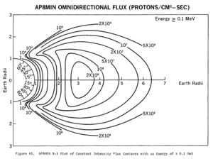  AP8 MIN omnidirectional proton flux ≥ 100 keV
  
• 

  AP8 MIN omnidirectional proton flux ≥ 1 MeV
  
• 

  AP8 MIN omnidirectional proton flux ≥ 400 MeV
  

Antimatter confinement

In 2011, a study confirmed earlier speculation that the Van Allen belt could confine antiparticles. The PAMELA experiment detected levels of antiprotons orders of magnitude higher than are expected from normal particle decays while passing through the South Atlantic Anomaly. This suggests the Van Allen belts confine a significant flux of antiprotons produced by the interaction of the Earth's upper atmosphere with cosmic rays. The energy of the antiprotons has been measured in the range from 60–750 MeV. 

Research funded by the NASA Institute for Advanced Concepts concluded that harnessing these antiprotons for spacecraft propulsion would be feasible. Researchers believed that this approach would have advantages over antiproton generation at CERN because collecting the particles in situ eliminates transportation losses and costs. Jupiter and Saturn are also possible sources but the Earth belt is the most productive. Jupiter is less productive than might be expected due to magnetic shielding from cosmic rays of much of its atmosphere. In 2019 CMS announced, that the construction of such device, which would be capable of collecting these particles has already begun. NASA will use this device to collect these particles and transport them to institutes all around the world for further examination. These so-called „Antimatter- Containers“ could be used for industrial purpose as well in the future.

Implications for space travel

Comparison of geostationary, GPS, GLONASS, Galileo, Compass (MEO), International Space Station, Hubble Space Telescope, Iridium constellation and graveyard orbits, with the Van Allen radiation belts and the Earth to scale. The Moon's orbit is around 9 times larger than geostationary orbit.

 

Spacecraft travelling beyond low Earth orbit enter the zone of radiation of the Van Allen belts. Beyond the belts, they face additional hazards from cosmic rays and solar particle events. A region between the inner and outer Van Allen belts lies at two to four Earth radii and is sometimes referred to as the "safe zone".

Solar cells, integrated circuits, and sensors can be damaged by radiation. Geomagnetic storms occasionally damage electronic components on spacecraft. Miniaturization and digitization of electronics and logic circuits have made satellites more vulnerable to radiation, as the total electric charge in these circuits is now small enough so as to be comparable with the charge of incoming ions. Electronics on satellites must be hardened against radiation to operate reliably. The Hubble Space Telescope, among other satellites, often has its sensors turned off when passing through regions of intense radiation. A satellite shielded by 3 mm of aluminium in an elliptic orbit (200 by 20,000 miles (320 by 32,190 km)) passing the radiation belts will receive about 2,500 rem (25 Sv) per year (for comparison, a full-body dose of 5 Sv is deadly). Almost all radiation will be received while passing the inner belt.

The Apollo missions marked the first event where humans traveled through the Van Allen belts, which was one of several radiation hazards known by mission planners. The astronauts had low exposure in the Van Allen belts due to the short period of time spent flying through them. Apollo flight trajectories bypassed the inner belts completely, passing through the thinner areas of the outer belts.

Astronauts' overall exposure was actually dominated by solar particles once outside Earth's magnetic field. The total radiation received by the astronauts varied from mission to mission but was measured to be between 0.16 and 1.14 rads (1.6 and 11.4 mGy), much less than the standard of 5 rem (50 mSv) per year set by the United States Atomic Energy Commission for people who work with radioactivity.

Causes

It is generally understood that the inner and outer Van Allen belts result from different processes. The inner belt, consisting mainly of energetic protons, is the product of the decay of so-called "albedo" neutrons which are themselves the result of cosmic ray collisions in the upper atmosphere. The outer belt consists mainly of electrons. They are injected from the geomagnetic tail following geomagnetic storms, and are subsequently energized through wave-particle interactions. 

In the inner belt, particles that originate from the Sun are trapped in the Earth's magnetic field. Particles spiral along the magnetic lines of flux as they move "longitudinally" along those lines. As particles move toward the poles, the magnetic field line density increases and their "longitudinal" velocity is slowed and can be reversed, reflecting the particle and causing them to bounce back and forth between the Earth's poles. In addition to the spiral about and motion along the flux lines, the electrons move slowly in an eastward direction, while the ions move westward. 

A gap between the inner and outer Van Allen belts, sometimes called safe zone or safe slot, is caused by the Very Low Frequency (VLF) waves which scatter particles in pitch angle which results in the gain of particles to the atmosphere. Solar outbursts can pump particles into the gap but they drain again in a matter of days. The radio waves were originally thought to be generated by turbulence in the radiation belts, but recent work by James L. Green of the Goddard Space Flight Center comparing maps of lightning activity collected by the Microlab 1 spacecraft with data on radio waves in the radiation-belt gap from the IMAGE spacecraft suggests that they are actually generated by lightning within Earth's atmosphere. The radio waves that generate strike the ionosphere at the correct angle to pass through only at high latitudes, where the lower ends of the gap approach the upper atmosphere. These results are still under scientific debate.

Proposed removal

High Voltage Orbiting Long Tether, or HiVOLT, is a concept proposed by Russian physicist V. V. Danilov and further refined by Robert P. Hoyt and Robert L. Forward for draining and removing the radiation fields of the Van Allen radiation belts that surround the Earth. A proposed configuration consists of a system of five 100 km long conducting tethers deployed from satellites, and charged to a large voltage. This would cause charged particles that encounter the tethers to have their pitch angle changed; thus, over time, dissolving the inner belts. Hoyt and Forward's company, Tethers Unlimited, performed a preliminary analysis simulation in 2011, and produced a chart depicting a theoretical radiation flux reduction, to less than 1% of current levels within two months for the inner belts that threaten LEO objects.

Cyclone

From Wikipedia, the free encyclopedia

 

An extratropical cyclone near Iceland on September 4, 2003

 

In meteorology, a cyclone is a large scale air mass that rotates around a strong center of low atmospheric pressure. Cyclones are characterized by inward spiraling winds that rotate about a zone of low pressure. The largest low-pressure systems are polar vortices and extratropical cyclones of the largest scale (the synoptic scale). Warm-core cyclones such as tropical cyclones and subtropical cyclones also lie within the synoptic scale. Mesocyclones, tornadoes, and dust devils lie within smaller mesoscale. Upper level cyclones can exist without the presence of a surface low, and can pinch off from the base of the tropical upper tropospheric trough during the summer months in the Northern Hemisphere. Cyclones have also been seen on extraterrestrial planets, such as Mars, Jupiter, and Neptune. Cyclogenesis is the process of cyclone formation and intensification. Extratropical cyclones begin as waves in large regions of enhanced mid-latitude temperature contrasts called baroclinic zones. These zones contract and form weather fronts as the cyclonic circulation closes and intensifies. Later in their life cycle, extratropical cyclones occlude as cold air masses undercut the warmer air and become cold core systems. A cyclone's track is guided over the course of its 2 to 6 day life cycle by the steering flow of the subtropical jet stream. 

Weather fronts mark the boundary between two masses of air of different temperature, humidity, and densities, and are associated with the most prominent meteorological phenomena. Strong cold fronts typically feature narrow bands of thunderstorms and severe weather, and may on occasion be preceded by squall lines or dry lines. Such fronts form west of the circulation center and generally move from west to east; warm fronts form east of the cyclone center and are usually preceded by stratiform precipitation and fog. Warm fronts move poleward ahead of the cyclone path. Occluded fronts form late in the cyclone life cycle near the center of the cyclone and often wrap around the storm center.

Tropical cyclogenesis describes the process of development of tropical cyclones. Tropical cyclones form due to latent heat driven by significant thunderstorm activity, and are warm core. Cyclones can transition between extratropical, subtropical, and tropical phases. Mesocyclones form as warm core cyclones over land, and can lead to tornado formation. Waterspouts can also form from mesocyclones, but more often develop from environments of high instability and low vertical wind shear. In the Atlantic and the northeastern Pacific oceans, a tropical cyclone is generally referred to as a hurricane (from the name of the ancient Central American deity of wind, Huracan), in the Indian and south Pacific oceans it is called a cyclone, and in the northwestern Pacific it is called a typhoon. The growth of instability in the vortices is not universal. For example, the size, intensity, moist-convection, surface evaporation, the value of potential temperature at each potential height can affect the nonlinear evolution of a vortex.

Nomenclature

Henry Piddington published 40 papers dealing with tropical storms from Calcutta between 1836 and 1855 in The Journal of the Asiatic Society. He also coined the term cyclone, meaning the coil of a snake. In 1842, he published his landmark thesis, Laws of the Storms.

Structure

Comparison between extratropical and tropical cyclones on surface analysis

 

There are a number of structural characteristics common to all cyclones. A cyclone is a low-pressure area. A cyclone's center (often known in a mature tropical cyclone as the eye), is the area of lowest atmospheric pressure in the region. Near the center, the pressure gradient force (from the pressure in the center of the cyclone compared to the pressure outside the cyclone) and the force from the Coriolis effect must be in an approximate balance, or the cyclone would collapse on itself as a result of the difference in pressure.

Because of the Coriolis effect, the wind flow around a large cyclone is counterclockwise in the Northern Hemisphere and clockwise in the Southern Hemisphere. In the Northern Hemisphere, the fastest winds relative to the surface of the Earth therefore occur on the eastern side of a northward-moving cyclone and on the northern side of a westward-moving one; the opposite occurs in the Southern Hemisphere. In contrast to low pressure systems, the wind flow around high pressure systems are clockwise (anticyclonic) in the northern hemisphere, and counterclockwise in the southern hemisphere.

Formation

The initial extratropical low-pressure area forms at the location of the red dot on the image. It is usually perpendicular (at a right angle to) the leaf-like cloud formation seen on satellite during the early stage of cyclogenesis. The location of the axis of the upper level jet stream is in light blue.

 

Tropical cyclones form when the energy released by the condensation of moisture in rising air causes a positive feedback loop over warm ocean waters.

Cyclogenesis is the development or strengthening of cyclonic circulation in the atmosphere. Cyclogenesis is an umbrella term for several different processes that all result in the development of some sort of cyclone. It can occur at various scales, from the microscale to the synoptic scale. 

Extratropical cyclones begin as waves along weather fronts before occluding later in their life cycle as cold-core systems. However, some intense extratropical cyclones can become warm-core systems when a warm seclusion occurs. 

Tropical cyclones form as a result of significant convective activity, and are warm core. Mesocyclones form as warm core cyclones over land, and can lead to tornado formation. Waterspouts can also form from mesocyclones, but more often develop from environments of high instability and low vertical wind shear. Cyclolysis is the opposite of cyclogenesis, and is the high-pressure system equivalent, which deals with the formation of high-pressure areas—Anticyclogenesis.

A surface low can form in a variety of ways. Topography can create a surface low. Mesoscale convective systems can spawn surface lows that are initially warm core. The disturbance can grow into a wave-like formation along the front and the low is positioned at the crest. Around the low, the flow becomes cyclonic. This rotational flow moves polar air towards the equator on the west side of the low, while warm air move towards the pole on the east side. A cold front appears on the west side, while a warm front forms on the east side. Usually, the cold front moves at a quicker pace than the warm front and "catches up" with it due to the slow erosion of higher density air mass out ahead of the cyclone. In addition, the higher density air mass sweeping in behind the cyclone strengthens the higher pressure, denser cold air mass. The cold front over takes the warm front, and reduces the length of the warm front. At this point an occluded front forms where the warm air mass is pushed upwards into a trough of warm air aloft, which is also known as a trowal.

Tropical cyclogenesis is the development and strengthening of a tropical cyclone. The mechanisms by which tropical cyclogenesis occurs are distinctly different from those that produce mid-latitude cyclones. Tropical cyclogenesis, the development of a warm-core cyclone, begins with significant convection in a favorable atmospheric environment. There are six main requirements for tropical cyclogenesis:

1. sufficiently warm sea surface temperatures,
2. atmospheric instability,
3. high humidity in the lower to middle levels of the troposphere
4. enough Coriolis force to develop a low-pressure center
5. a preexisting low-level focus or disturbance
6. low vertical wind shear.

An average of 86 tropical cyclones of tropical storm intensity form annually worldwide, with 47 reaching hurricane/typhoon strength, and 20 becoming intense tropical cyclones (at least Category 3 intensity on the Saffir–Simpson Hurricane Scale).

Synoptic scale

A fictitious synoptic chart of an extratropical cyclone affecting the UK and Ireland. The blue arrows between isobars indicate the direction of the wind, while the "L" symbol denotes the centre of the "low". Note the occluded, cold and warm frontal boundaries.

 

The following types of cyclones are identifiable in synoptic charts.

Surface-based types

There are three main types of surface-based cyclones: Extratropical cyclones, Subtropical cyclones and Tropical cyclones

Extratropical cyclone

An extratropical cyclone is a synoptic scale of low-pressure weather system that does not have tropical characteristics, as it is connected with fronts and horizontal gradients (rather than vertical) in temperature and dew point otherwise known as "baroclinic zones".

"Extratropical" is applied to cyclones outside the tropics, in the middle latitudes. These systems may also be described as "mid-latitude cyclones" due to their area of formation, or "post-tropical cyclones" when a tropical cyclone has moved (extratropical transition) beyond the tropics. They are often described as "depressions" or "lows" by weather forecasters and the general public. These are the everyday phenomena that, along with anti-cyclones, drive weather over much of the Earth. 

Although extratropical cyclones are almost always classified as baroclinic since they form along zones of temperature and dewpoint gradient within the westerlies, they can sometimes become barotropic late in their life cycle when the temperature distribution around the cyclone becomes fairly uniform with radius. An extratropical cyclone can transform into a subtropical storm, and from there into a tropical cyclone, if it dwells over warm waters sufficient to warm its core, and as a result develops central convection. A particularly intense type of extratropical cyclone that strikes during winter is known colloquially as a nor'easter.

Polar low

A polar low over the Sea of Japan in December 2009

 

A polar low is a small-scale, short-lived atmospheric low-pressure system (depression) that is found over the ocean areas poleward of the main polar front in both the Northern and Southern Hemispheres. Polar lows were first identified on the meteorological satellite imagery that became available in the 1960s, which revealed many small-scale cloud vortices at high latitudes. The most active polar lows are found over certain ice-free maritime areas in or near the Arctic during the winter, such as the Norwegian Sea, Barents Sea, Labrador Sea and Gulf of Alaska. Polar lows dissipate rapidly when they make landfall. Antarctic systems tend to be weaker than their northern counterparts since the air-sea temperature differences around the continent are generally smaller. However, vigorous polar lows can be found over the Southern Ocean. During winter, when cold-core lows with temperatures in the mid-levels of the troposphere reach −45 °C (−49 °F) move over open waters, deep convection forms, which allows polar low development to become possible. The systems usually have a horizontal length scale of less than 1,000 kilometres (620 mi) and exist for no more than a couple of days. They are part of the larger class of mesoscale weather systems. Polar lows can be difficult to detect using conventional weather reports and are a hazard to high-latitude operations, such as shipping and gas and oil platforms. Polar lows have been referred to by many other terms, such as polar mesoscale vortex, Arctic hurricane, Arctic low, and cold air depression. Today the term is usually reserved for the more vigorous systems that have near-surface winds of at least 17 m/s.

Subtropical

Subtropical Storm Alex in the north Atlantic Ocean in January 2016

A subtropical cyclone is a weather system that has some characteristics of a tropical cyclone and some characteristics of an extratropical cyclone. They can form between the equator and the 50th parallel. As early as the 1950s, meteorologists were unclear whether they should be characterized as tropical cyclones or extratropical cyclones, and used terms such as quasi-tropical and semi-tropical to describe the cyclone hybrids. By 1972, the National Hurricane Center officially recognized this cyclone category. Subtropical cyclones began to receive names off the official tropical cyclone list in the Atlantic Basin in 2002. They have broad wind patterns with maximum sustained winds located farther from the center than typical tropical cyclones, and exist in areas of weak to moderate temperature gradient.

Since they form from extratropical cyclones, which have colder temperatures aloft than normally found in the tropics, the sea surface temperatures required is around 23 degrees Celsius (73 °F) for their formation, which is three degrees Celsius (5 °F) lower than for tropical cyclones. This means that subtropical cyclones are more likely to form outside the traditional bounds of the hurricane season. Although subtropical storms rarely have hurricane-force winds, they may become tropical in nature as their cores warm.

Tropical

2017 Atlantic hurricane season summary map

 

A tropical cyclone is a storm system characterized by a low-pressure center and numerous thunderstorms that produce strong winds and flooding rain. A tropical cyclone feeds on heat released when moist air rises, resulting in condensation of water vapour contained in the moist air. They are fueled by a different heat mechanism than other cyclonic windstorms such as nor'easters, European windstorms, and polar lows, leading to their classification as "warm core" storm systems.

Hurricane Catarina, a rare South Atlantic tropical cyclone viewed from the International Space Station on March 26, 2004

 

The term "tropical" refers to both the geographic origin of these systems, which form almost exclusively in tropical regions of the globe, and their dependence on Maritime Tropical air masses for their formation. The term "cyclone" refers to the storms' cyclonic nature, with counterclockwise rotation in the Northern Hemisphere and clockwise rotation in the Southern Hemisphere. Depending on their location and strength, tropical cyclones are referred to by other names, such as hurricane, typhoon, tropical storm, cyclonic storm, tropical depression, or simply as a cyclone.

While tropical cyclones can produce extremely powerful winds and torrential rain, they are also able to produce high waves and a damaging storm surge. Their winds increase the wave size, and in so doing they draw more heat and moisture into their system, thereby increasing their strength. They develop over large bodies of warm water, and hence lose their strength if they move over land. This is the reason coastal regions can receive significant damage from a tropical cyclone, while inland regions are relatively safe from strong winds. Heavy rains, however, can produce significant flooding inland. Storm surges are rises in sea level caused by the reduced pressure of the core that in effect "sucks" the water upward and from winds that in effect "pile" the water up. Storm surges can produce extensive coastal flooding up to 40 kilometres (25 mi) from the coastline. Although their effects on human populations can be devastating, tropical cyclones can also relieve drought conditions. They also carry heat and energy away from the tropics and transport it toward temperate latitudes, which makes them an important part of the global atmospheric circulation mechanism. As a result, tropical cyclones help to maintain equilibrium in the Earth's troposphere. 

Many tropical cyclones develop when the atmospheric conditions around a weak disturbance in the atmosphere are favorable. Others form when other types of cyclones acquire tropical characteristics. Tropical systems are then moved by steering winds in the troposphere; if the conditions remain favorable, the tropical disturbance intensifies, and can even develop an eye. On the other end of the spectrum, if the conditions around the system deteriorate or the tropical cyclone makes landfall, the system weakens and eventually dissipates. A tropical cyclone can become extratropical as it moves toward higher latitudes if its energy source changes from heat released by condensation to differences in temperature between air masses. A tropical cyclone is usually not considered to become subtropical during its extratropical transition.

Upper level types

Polar cyclone

A polar, sub-polar, or Arctic cyclone (also known as a polar vortex) is a vast area of low pressure that strengthens in the winter and weakens in the summer. A polar cyclone is a low-pressure weather system, usually spanning 1,000 kilometres (620 mi) to 2,000 kilometres (1,200 mi), in which the air circulates in a counterclockwise direction in the northern hemisphere, and a clockwise direction in the southern hemisphere. The Coriolis acceleration acting on the air masses moving poleward at high altitude, causes a counterclockwise circulation at high altitude. The poleward movement of air originates from the air circulation of the Polar cell. The polar low is not driven by convection as are tropical cyclones, nor the cold and warm air mass interactions as are extratropical cyclones, but is an artifact of the global air movement of the Polar cell. The base of the polar low is in the mid to upper troposphere. In the Northern Hemisphere, the polar cyclone has two centers on average. One center lies near Baffin Island and the other over northeast Siberia. In the southern hemisphere, it tends to be located near the edge of the Ross ice shelf near 160 west longitude. When the polar vortex is strong, its effect can be felt at the surface as a westerly wind (toward the east). When the polar cyclone is weak, significant cold outbreaks occur.

TUTT cell

Under specific circumstances, upper level cold lows can break off from the base of the Tropical Upper Tropospheric Trough (TUTT), which is located mid-ocean in the Northern Hemisphere during the summer months. These upper tropospheric cyclonic vortices, also known as TUTT cells or TUTT lows, usually move slowly from east-northeast to west-southwest, and their bases generally do not extend below 20,000 feet (6,100 m) in altitude. A weak inverted surface trough within the trade wind is generally found underneath them, and they may also be associated with broad areas of high-level clouds. Downward development results in an increase of cumulus clouds and the appearance of a surface vortex. In rare cases, they become warm-core tropical cyclones. Upper cyclones and the upper troughs that trail tropical cyclones can cause additional outflow channels and aid in their intensification. Developing tropical disturbances can help create or deepen upper troughs or upper lows in their wake due to the outflow jet emanating from the developing tropical disturbance/cyclone.

Mesoscale

The following types of cyclones are not identifiable in synoptic charts.

Mesocyclone

A mesocyclone is a vortex of air, 2.0 kilometres (1.2 mi) to 10 kilometres (6.2 mi) in diameter (the mesoscale of meteorology), within a convective storm. Air rises and rotates around a vertical axis, usually in the same direction as low-pressure systems in both northern and southern hemisphere. They are most often cyclonic, that is, associated with a localized low-pressure region within a supercell. Such storms can feature strong surface winds and severe hail. Mesocyclones often occur together with updrafts in supercells, where tornadoes may form. About 1,700 mesocyclones form annually across the United States, but only half produce tornadoes.

Tornado

A tornado is a violently rotating column of air that is in contact with both the surface of the earth and a cumulonimbus cloud or, in rare cases, the base of a cumulus cloud. Also referred to as twisters, a colloquial term in America, or cyclones, although the word cyclone is used in meteorology, in a wider sense, to name any closed low-pressure circulation.

Dust devil

A dust devil is a strong, well-formed, and relatively long-lived whirlwind, ranging from small (half a metre wide and a few metres tall) to large (more than 10 metres wide and more than 1000 metres tall). The primary vertical motion is upward. Dust devils are usually harmless, but can on rare occasions grow large enough to pose a threat to both people and property.

Waterspout

A waterspout is a columnar vortex forming over water that is, in its most common form, a non-supercell tornado over water that is connected to a cumuliform cloud. While it is often weaker than most of its land counterparts, stronger versions spawned by mesocyclones do occur.

Steam devil

A gentle vortex over calm water or wet land made visible by rising water vapour.

Fire whirl

A fire whirl – also colloquially known as a fire devil, fire tornado, firenado, or fire twister – is a whirlwind induced by a fire and often made up of flame or ash.

Climate change

Scientists warn that climate change could increase the intensity of typhoons as climate change projections show that the difference in temperature between the ocean – the heat source for cyclones – and the storm tops – the cold parts of cyclones – are likely to increase. Climate change is predicted to increase the frequency of high-intensity storms in selected ocean basins. While the effect changing climate is having on tropical storms remains largely unresolved scientists and president of Vanuatu Baldwin Lonsdale say the devastation caused by Pam, was aggravated by climate change.

Other planets

Cyclone on Mars, imaged by the Hubble Space Telescope

 

Cyclones are not unique to Earth. Cyclonic storms are common on Jovian planets, such as the Small Dark Spot on Neptune. It is about one third the diameter of the Great Dark Spot and received the nickname "Wizard's Eye" because it looks like an eye. This appearance is caused by a white cloud in the middle of the Wizard's Eye. Mars has also exhibited cyclonic storms. Jovian storms like the Great Red Spot are usually mistakenly named as giant hurricanes or cyclonic storms. However, this is inaccurate, as the Great Red Spot is, in fact, the inverse phenomenon, an anticyclone.

SETI@home

From Wikipedia, the free encyclopedia

SETI@home

Developer(s)	University Of California, Berkeley
Initial release	May 17, 1999
Stable release	SETI@home v8：8.00 / December 30, 2015; 3 years ago SETI@home v8 for nVidia and AMD/ATi GPU Card：8.12/ May 19, 2016; 3 years ago AstroPulse v7：7.00/ October 7, 2014; 4 years ago AstroPulse v7 for nVidia and AMD/ATi GPU Card：7.10/ April 23, 2015; 4 years ago
Development status	Online
Project goal(s)	Discovery of radio evidence of extraterrestrial life
Funding	Public funding and private donations
Operating system	Microsoft Windows, Linux, Android, macOS, Solaris, IBM AIX, FreeBSD, DragonflyBSD, OpenBSD, NetBSD, HP-UX, IRIX, Tru64 Unix, OS/2 Warp, eComStation
Platform	Cross-platform
Available in	English
Type	Volunteer computing
License	GPL
Active users	103,480 (January 2018)
Total users	1,716,012 (January 2018)
Website	SETI@home

SETI@home ("SETI at home") is an Internet-based public volunteer computing project employing the BOINC software platform created by the Berkeley SETI Research Center and is hosted by the Space Sciences Laboratory, at the University of California, Berkeley. Its purpose is to analyze radio signals, searching for signs of extraterrestrial intelligence, and as such is one of many activities undertaken as part of the worldwide SETI effort.

SETI@home was released to the public on May 17, 1999, making it the third large-scale use of distributed computing over the Internet for research purposes, after Great Internet Mersenne Prime Search (GIMPS) was launched in 1996 and distributed.net in 1997. Along with MilkyWay@home and Einstein@home, it is the third major computing project of this type that has the investigation of phenomena in interstellar space as its primary purpose.

Scientific research

The two original goals of SETI@home were:

• to do useful scientific work by supporting an observational analysis to detect intelligent life outside Earth
• to prove the viability and practicality of the "volunteer computing" concept

The second of these goals is considered to have succeeded completely. The current BOINC environment, a development of the original SETI@home, is providing support for many computationally intensive projects in a wide range of disciplines.

The first of these goals has to date yielded no conclusive results: no evidence for ETI signals has been shown via SETI@home. However, the ongoing continuation is predicated on the assumption that the observational analysis is not an "ill-posed" one. The remainder of this article deals specifically with the original SETI@home observations/analysis. The vast majority of the sky (over 98%) has yet to be surveyed, and each point in the sky must be surveyed many times to exclude even a subset of possibilities.

Procedure details

SETI@home searches for possible evidence of radio transmissions from extraterrestrial intelligence using observational data from the Arecibo radio telescope and the Green Bank Telescope. The data is taken "piggyback" or "passively" while the telescope is used for other scientific programs. The data is digitized, stored, and sent to the SETI@home facility. The data are then parsed into small chunks in frequency and time, and analyzed, using software, to search for any signals—that is, variations which cannot be ascribed to noise, and hence contain information. Using distributed computing, SETI@home sends the millions of chunks of data to be analyzed off-site by home computers, and then have those computers report the results. Thus what appears a difficult problem in data analysis is reduced to a reasonable one by aid from a large, Internet-based community of borrowed computer resources. 

The software searches for five types of signals that distinguish them from noise:

• Spikes in power spectra
• Gaussian rises and falls in transmission power, possibly representing the telescope beam's main lobe passing over a radio source
• Triplets — three power spikes in a row
• Pulsing signals that possibly represent a narrowband digital-style transmission
• Autocorrelation detects signal waveforms.

There are many variations on how an ETI signal may be affected by the interstellar medium, and by the relative motion of its origin compared to Earth. The potential "signal" is thus processed in many ways (although not testing all detection methods nor scenarios) to ensure the highest likelihood of distinguishing it from the scintillating noise already present in all directions of outer space. For instance, another planet is very likely to be moving at a speed and acceleration with respect to Earth, and that will shift the frequency, over time, of the potential "signal." Checking for this through processing is done, to an extent, in the SETI@home software. 

The process is somewhat like tuning a radio to various channels, and looking at the signal strength meter. If the strength of the signal goes up, that gets attention. More technically, it involves a lot of digital signal processing, mostly discrete Fourier transforms at various chirp rates and durations.

Results

To date, the project has not confirmed the detection of any ETI signals. However, it has identified several candidate targets (sky positions), where the spike in intensity is not easily explained as noisespots, for further analysis. The most significant candidate signal to date was announced on September 1, 2004, named Radio source SHGb02+14a. 

While the project has not reached the stated primary goal of finding extraterrestrial intelligence, it has proved to the scientific community that distributed computing projects using Internet-connected computers can succeed as a viable analysis tool, and even beat the largest supercomputers. However, it has not been demonstrated that the order of magnitude excess in computers used, many outside the home (the original intent was to use 50,000-100,000 "home" computers), has benefited the project scientifically. (For more on this, see § Challenges to the project below.)

Astronomer Seth Shostak stated in 2004 that he expects to get a conclusive signal and proof of alien contact between 2020 and 2025, based on the Drake equation. This implies that a prolonged effort may benefit SETI@home, despite its (present) twenty-year run without success in ETI detection.

Technology

Anybody with an at least intermittently Internet-connected computer can participate in SETI@home by running a free program that downloads and analyzes radio telescope data.

Observational data are recorded on 2-terabyte SATA hard disk drives at the Arecibo Observatory in Puerto Rico, each holding about 2.5 days of observations, which are then sent to Berkeley. Arecibo does not have a broadband Internet connection, so data must go by postal mail to Berkeley. Once there, it is divided in both time and frequency domains work units of 107 seconds of data, or approximately 0.35 megabytes (350 kilobytes or 350,000 bytes), which overlap in time but not in frequency. These work units are then sent from the SETI@home server over the Internet to personal computers around the world to analyze.

The analysis software can search for signals with about one-tenth the strength of those sought in previous surveys, because it makes use of a computationally-intensive algorithm called coherent integration that no one else has had the computing power to implement.

Data is merged into a database using SETI@home computers in Berkeley. Interference is rejected, and various pattern-detection algorithms are applied to search for the most interesting signals. 

The project uses CUDA for GPU processing since 2015.

Since 2016, the project has also been helping to process data from the Breakthrough Listen project which has been recorded at Green Bank Telescope.

Software

The BOINC Manager working on the SETI@home project (v 7.6.22).

 

Screenshot of SETI@home Enhanced BOINC Screensaver (v6.03)

 

Screenshot of SETI@home Classic Screensaver (v3.07)

 

The SETI@home distributed computing software runs either as a screensaver or continuously while a user works, making use of processor time that would otherwise be unused. 

The initial software platform, now referred to as "SETI@home Classic," ran from May 17, 1999, to December 15, 2005. This program was only capable of running SETI@home; it was replaced by Berkeley Open Infrastructure for Network Computing (BOINC), which also allows users to contribute to other distributed computing projects at the same time as running SETI@home. The BOINC platform will also allow testing for more types of signals.

The discontinuation of the SETI@home Classic platform has rendered older Macintosh computers running the classic Mac OS unsuitable for participating in the project.

SETI@home is available for the Sony PlayStation 3 console.

On May 3, 2006, new work units for a new version of SETI@home called "SETI@home Enhanced" started distribution. Since computers now have the power for more computationally intensive work than when the project began, this new version is more sensitive by a factor of two concerning Gaussian signals and to some kinds of pulsed signals than the original SETI@home (BOINC) software. This new application has been optimized to the point where it will run faster on some work units than earlier versions. However, some work units (the best work units, scientifically speaking) will take significantly longer. 

In addition, some distributions of the SETI@home applications have been optimized for a particular type of CPU. They are referred to as "optimized executables" and have been found to run faster on systems specific for that CPU. As of 2007, most of these applications are optimized for Intel processors and their corresponding instruction sets.

The results of the data processing are normally automatically transmitted when the computer is next connected to the Internet; it can also be instructed to connect to the Internet as needed.

Statistics

With over 5.2 million participants worldwide, the project is the distributed computing project with the most participants to date. The original intent of SETI@home was to utilize 50,000-100,000 home computers. Since its launch on May 17, 1999, the project has logged over two million years of aggregate computing time. On September 26, 2001, SETI@home had performed a total of 10²¹ floating point operations. It was acknowledged by the 2008 edition of the Guinness World Records as the largest computation in history. With over 145,000 active computers in the system (1.4 million total) in 233 countries, as of 23 June 2013, SETI@home had the ability to compute over 668 teraFLOPS. For comparison, the Tianhe-2 computer, which as of 23 June 2013 was the world's fastest supercomputer, was able to compute 33.86 petaFLOPS (approximately 50 times greater).

Project future

There were plans to get data from the Parkes Observatory in Australia to analyze the southern hemisphere. However, as of 3 June 2018, these plans were not mentioned in the project's website. Other plans include a Multi-Beam Data Recorder, a Near Time Persistency Checker and Astropulse (an application that uses coherent dedispersion to search for pulsed signals). Astropulse will team with the original SETI@home to detect other sources, such as rapidly rotating pulsars, exploding primordial black holes, or as-yet unknown astrophysical phenomena. Beta testing of the final public release version of Astropulse was completed in July 2008, and the distribution of work units to higher spec machines capable of processing the more CPU intensive work units started in mid-July 2008.

Competitive aspect

SETI@home users quickly started to compete with one another to process the maximum number of work units. Teams were formed to combine the efforts of individual users. The competition continued and grew larger with the introduction of BOINC. 

As with any competition, attempts have been made to "cheat" the system and claim credit for work that has not been performed. To combat cheats, the SETI@home system sends every work unit to multiple computers, a value known as "initial replication" (currently 2). Credit is only granted for each returned work unit once a minimum number of results have been returned and the results agree, a value known as "minimum quorum" (currently 2). If, due to computation errors or cheating by submitting false data, not enough results agree, more identical work units are sent out until the minimum quorum can be reached. The final credit granted to all machines which returned the correct result is the same and is the lowest of the values claimed by each machine. The claimed credit by each machine for an identical work unit often varies due to minor differences in floating point arithmetic on different processors.

Some users have installed and run SETI@home on computers at their workplaces — an act known as "Borging", after the assimilation-driven Borg of Star Trek. In some cases, SETI@home users have misused company resources to gain work-unit results — with at least two individuals getting fired for running SETI@home on an enterprise production system. There is a thread in the newsgroup alt.sci.seti which bears the title "Anyone fired for SETI screensaver" and ran starting as early as September 14, 1999. 

Other users collect large quantities of equipment together at home to create "SETI farms", which typically consist of a number of computers consisting of only a motherboard, CPU, RAM and power supply that are arranged on shelves as diskless workstations running either Linux or old versions of Microsoft Windows "headless" (without a monitor).

Challenges to the project

There are other challenges to the project's future viability. 

Like any project of prolonged duration, there are factors that may result in its termination. Some of these are detailed below:

Potential closure of Arecibo Observatory

At present, SETI@home procures its data from the Arecibo Observatory facility operated by the National Astronomy and Ionosphere Center and administered by SRI International. 

The decreasing operating budget for the observatory has created a shortfall of funds which has not been made up from other sources such as private donors, NASA, other foreign research institutions, nor private non-profit organizations such as SETI@home. 

However, in the overall longterm views held by many involved with the SETI project, any usable radio telescope could take over from Arecibo, as all the SETI systems are portable and relocatable.

Alternative distributed computing projects

When the project launched, there were few alternative ways of donating computer time to research projects. However, there are now many other projects that are competing for such time.

More restrictive computer use policies in businesses

In one documented case, an individual was fired for explicitly importing and using the SETI@home software on computers used for the U.S. state of Ohio. In another incident a school IT director resigned after his installation allegedly cost his school district $1 million in removal costs; however, other reasons for this firing included lack of communication with his superiors, not installing firewall software and alleged theft of computer equipment, leading a ZDNet editor to comment that "the distributed computing nonsense was simply the best and most obvious excuse the district had to terminate his contract with cause".

As of 16 October 2005, approximately one-third of the processing for the non-BOINC version of the software was performed on work or school based machines. As many of these computers will give reduced privileges to ordinary users, it is possible that much of this has been done by network administrators. 

To some extent, this may be offset by better connectivity to home machines and increasing performance of home computers, especially those with GPUs, which have also benefited other distributed computing projects such as Folding@Home. The spread of mobile computing devices provides another large resource for distributed computing. For example, in 2012, Piotr Luszczek (a former doctoral student of Jack Dongarra), presented results showing that an iPad 2 matched the historical performance of a Cray-2 (the fastest computer in the world in 1985) on an embedded LINPACK benchmark.

Funding

There is currently no government funding for SETI research, and private funding is always limited. Berkeley Space Science Lab has found ways of working with small budgets, and the project has received donations allowing it to go well beyond its original planned duration, but it still has to compete for limited funds with other SETI projects and other space sciences projects. 

In a December 16, 2007 plea for donations, SETI@home stated its present modest state and urged donations of $476,000 needed for continuation into 2008.

Unofficial clients

A number of individuals and companies made unofficial changes to the distributed part of the software to try to produce faster results, but this compromised the integrity of all the results. As a result, the software had to be updated to make it easier to detect such changes, and discover unreliable clients. BOINC will run on unofficial clients; however, clients that return different and therefore incorrect data are not allowed, so corrupting the result database is avoided. BOINC relies on cross-checking to validate data but unreliable clients need to be identified, to avoid situations when two of these report the same invalid data and therefore corrupt the database. A very popular unofficial client (lunatic) allows users to take advantage of the special features provided by their processor(s) such as SSE, SSE2, SSE3, SSSE3, SSE4.1, and AVX to allow for faster processing. The only downside to this is that if the user selects features that their processor(s) do not support, the chances of bad results and crashes rise significantly. Tools (such as CPU-Z) are freely available to tell users what features are supported by their processor(s).

Hardware and database failures

SETI@home is a test bed for further development not only of BOINC but of other hardware and software (database) technology. Under SETI@home processing loads, these experimental technologies can be more challenging than expected, as SETI databases do not have typical accounting and business data or relational structures. The non-traditional database uses often do incur greater processing overheads and risk of database corruption and outright database failure. Hardware, software and database failures can (and do) cause dips in project participation.

The project has had to shut down several times to change over to new databases capable of handling more massive datasets. Hardware failure has proven to be a substantial source of project shutdowns—as hardware failure is often coupled with database corruption.