Transcranial magnetic stimulation

From Wikipedia, the free encyclopedia

Transcranial magnetic stimulation
Transcranial magnetic stimulation (schematic diagram)
MeSH	D050781

Transcranial magnetic stimulation (TMS) is a method in which a changing magnetic field is used to cause electric current to flow in a small region of the brain via electromagnetic induction. During a TMS procedure, a magnetic field generator, or "coil", is placed near the head of the person receiving the treatment.^[1]:3 The coil is connected to a pulse generator, or stimulator, that delivers a changing electric current to the coil.^[2]

TMS is used diagnostically to measure the connection between the central nervous system and skeletal muscle to evaluate damage in a wide variety of disease states, including stroke, multiple sclerosis, amyotrophic lateral sclerosis, movement disorders, and motor neuron diseases.^[3]

Evidence suggests it is useful for neuropathic pain^[4] and treatment-resistant major depressive disorder.^[4][5] A 2015 Cochrane review found that there was not enough evidence to determine its effectiveness in treating schizophrenia.^[6] For negative symptoms another review found possible efficacy.^[4] As of 2014, all other investigated uses of repetitive TMS have only possible or no clinical efficacy.^[4]

Matching the discomfort of TMS to distinguish true effects from placebo is an important and challenging issue that influences the results of clinical trials.^[4][7][8][9] Adverse effects of TMS are uncommon, and include fainting and rarely seizure.^[7] Other adverse effects of TMS include discomfort or pain, hypomania, cognitive changes, hearing loss, and inadvertent current induction in implanted devices such as pacemakers or defibrillators.^[7]

Medical uses

The use of TMS can be divided into diagnostic and therapeutic uses.

Diagnosis

TMS can be used clinically to measure activity and function of specific brain circuits in humans.^[3] The most robust and widely accepted use is in measuring the connection between the primary motor cortex and a muscle to evaluate damage from stroke, multiple sclerosis, amyotrophic lateral sclerosis, movement disorders, motor neuron disease and injuries and other disorders affecting the facial and other cranial nerves and the spinal cord.^{[3][10][11][12]} TMS has been suggested as a means of assessing short-interval intracortical inhibition (SICI) which measures the internal pathways of the motor cortex but this use has not yet been validated.^[13]

Treatment

For neuropathic pain, for which there is little effective treatment, high-frequency (HF) repetitive TMS (rTMS) appears effective.^[4] For treatment-resistant major depressive disorder, HF-rTMS of the left dorsolateral prefrontal cortex (DLPFC) appears effective and low-frequency (LF) rTMS of the right DLPFC has probable efficacy.^[4][5] The Royal Australia and New Zealand College of Psychiatrists has endorsed rTMS for treatment resistant MDD.^[14] As of October 2008, the US Food and Drug Administration authorized the use of rTMS as an effective treatment for clinical depression.^[15]

Adverse effects

Although TMS is generally regarded as safe, risks increase for therapeutic rTMS compared to single or paired TMS for diagnostic purposes.^[16] In the field of therapeutic TMS, risks increase with higher frequencies.^[7]

The greatest immediate risk is the rare occurrence of syncope (fainting) and even less commonly, induced seizures.^[7][17]

Other adverse short-term effects of TMS include discomfort or pain, transient induction of hypomania, transient cognitive changes, transient hearing loss, transient impairment of working memory, and induced currents in electrical circuits in implanted devices.^[7]

Devices and procedure

During a transcranial magnetic stimulation (TMS) procedure, a magnetic field generator, or "coil" is placed near the head of the person receiving the treatment.^[1]:3 The coil produces small electric currents in the region of the brain just under the coil via electromagnetic induction. The coil is positioned by finding anatomical landmarks on the skull including, but not limited to, the inion or the nasion.^[18] The coil is connected to a pulse generator, or stimulator, that delivers electric current to the coil.^[2]

Most devices provide a shallow magnetic field that affects neurons mostly on the surface of the brain, delivered with coil shaped like the number eight. Some devices can provide magnetic fields that can penetrate deeper, are used for "deep TMS", and have different types of coils including the H-coil the C-core coil, and the circular crown coil; as of 2013 the H coil used in devices made by Brainsway were the most developed.^[19]

Theta-burst stimulation

Theta-burst stimulation (TBS) is a popular protocol, as opposed to stimulation patterns based on other neural oscillation patterns (e.g. alpha-burst) used in transcranial magnetic stimulation. It was originally described by Huang in 2005.^[20] The protocol has been used clinical for multiple types of disorders. A specific example, for major depressive disorder with stimulation of both right and left dorsolateral prefrontal cortex (DLPFC) is as follows: The left is stimulated intermediately (iTBS) while the right is inhibited via continuous stimulation (cTBS). In the theta-burst stimulation pattern, 3 pulses are administered at 50 Hz, every 200 ms. In the intermittent theta burst stimulation pattern (iTBS), a 2-second train of TBS is repeated every 10 s for a total of 190 s (600 pulses). In the continuous theta burst stimulation paradigm (cTBS), a 40 s train of uninterrupted TBS is given (600 pulses).

In a March 2015 publication, Bakker^[21] demonstrated with 185 patients evenly divided between the standard 10 Hz protocol (30 min) and the theta-burst stimulation, that the outcome (reduction of Ham-D and BDI scores) was the same.

Society and culture

Regulatory approvals

Neurosurgery planning

Nexstim obtained 510(k) FDA clearance for the assessment of the primary motor cortex for pre-procedural planning in December 2009^[22] and for neurosurgical planning in June 2011.^[23]

Depression

A number of deep TMS have received FDA 510k clearance to market for use in adults with treatment resistant major depressive disorders.^{[24][25][26][27][28]}

Migraine

The use of single-pulse TMS was approved by the FDA for treatment of migraines in December 2013.^[29] It is approved as a Class II medical device under the "de novo pathway".^[30][31]

Others

In the European Economic Area, various versions of Deep TMS H-coils has CE marking for Alzheimer's disease,^[32] autism,^[32] bipolar disorder,^[33] epilepsy ^[34] chronic pain^[33] major depressive disorder^[33] Parkinson's disease,^[33][35] posttraumatic stress disorder (PTSD),^[33] schizophrenia (negative symptoms)^[33] and to aid smoking cessation.^[32] One review found tentative benefit for cognitive enhancement in healthy people.^[36]

Health insurance

United States

Commercial health insurance

In 2013, several commercial health insurance plans in the United States, including Anthem, Health Net, and Blue Cross Blue Shield of Nebraska and of Rhode Island, covered TMS for the treatment of depression for the first time.^[37] In contrast, UnitedHealthcare issued a medical policy for TMS in 2013 that stated there is insufficient evidence that the procedure is beneficial for health outcomes in patients with depression. UnitedHealthcare noted that methodological concerns raised about the scientific evidence studying TMS for depression include small sample size, lack of a validated sham comparison in randomized controlled studies, and variable uses of outcome measures.^[38] Other commercial insurance plans whose 2013 medical coverage policies stated that the role of TMS in the treatment of depression and other disorders had not been clearly established or remained investigational included Aetna, Cigna and Regence.^[39]

Medicare

Policies for Medicare coverage vary among local jurisdictions within the Medicare system,^[40] and Medicare coverage for TMS has varied among jurisdictions and with time. For example:

• In early 2012 in New England, Medicare covered TMS for the first time in the United States.^[41] However, that jurisdiction later decided to end coverage after October, 2013.^[42]
• In August 2012, the jurisdiction covering Arkansas, Louisiana, Mississippi, Colorado, Texas, Oklahoma, and New Mexico determined that there was insufficient evidence to cover the treatment,^[43] but the same jurisdiction subsequently determined that Medicare would cover TMS for the treatment of depression after December 2013.^[44]

United Kingdom's National Health Service

The United Kingdom's National Institute for Health and Care Excellence (NICE) issues guidance to the National Health Service (NHS) in England, Wales, Scotland and Northern Ireland. NICE guidance does not cover whether or not the NHS should fund a procedure. Local NHS bodies (primary care trusts and hospital trusts) make decisions about funding after considering the clinical effectiveness of the procedure and whether the procedure represents value for money for the NHS.^[45]

NICE evaluated TMS for severe depression (IPG 242) in 2007, and subsequently considered TMS for reassessment in January 2011 but did not change its evaluation.^[46] The Institute found that TMS is safe, but there is insufficient evidence for its efficacy.^[46]

In January 2014, NICE reported the results of an evaluation of TMS for treating and preventing migraine (IPG 477). NICE found that short-term TMS is safe but there is insufficient evidence to evaluate safety for long-term and frequent uses. It found that evidence on the efficacy of TMS for the treatment of migraine is limited in quantity, that evidence for the prevention of migraine is limited in both quality and quantity.^[47]

Technical information

TMS – Butterfly Coils

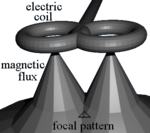
TMS uses electromagnetic induction to generate an electric current across the scalp and skull without physical contact.^[48] A plastic-enclosed coil of wire is held next to the skull and when activated, produces a magnetic field oriented orthogonally to the plane of the coil. The magnetic field passes unimpeded through the skin and skull, inducing an oppositely directed current in the brain that activates nearby nerve cells in much the same way as currents applied directly to the cortical surface.^[49]

The path of this current is difficult to model because the brain is irregularly shaped and electricity and magnetism are not conducted uniformly throughout its tissues. The magnetic field is about the same strength as an MRI, and the pulse generally reaches no more than 5 centimeters into the brain unless using the deep transcranial magnetic stimulation variant of TMS.^[50] Deep TMS can reach up to 6 cm into the brain to stimulate deeper layers of the motor cortex, such as that which controls leg motion.^[51]

Mechanism of action

${\displaystyle \mathbf {B} ={\frac {\mu _{0}}{4\pi }}I\int _{C}{\frac {d\mathbf {l} \times \mathbf {\hat {r}} }{r^{2}}}}$
it has been shown that a current through a wire generates a magnetic field around that wire. Transcranial magnetic stimulation is achieved by quickly discharging current from a large capacitor into a coil to produce pulsed magnetic fields between 2 and 3 T.^[52] By directing the magnetic field pulse at a targeted area of the brain, one can either depolarize or hyperpolarize neurons in the brain. The magnetic flux density pulse generated by the current pulse through the coil causes an electric field as explained by the Maxwell-Faraday equation,

${\displaystyle \nabla \times \mathbf {E} =-{\frac {\partial \mathbf {B} }{\partial t}}}$ .
This electric field causes a change in the transmembrane current of the neuron, which leads to the depolarization or hyperpolarization of the neuron and the firing of an action potential.^[52]

The exact details of how TMS functions are still being explored. The effects of TMS can be divided into two types depending on the mode of stimulation:

• Single or paired pulse TMS causes neurons in the neocortex under the site of stimulation to depolarize and discharge an action potential. If used in the primary motor cortex, it produces muscle activity referred to as a motor evoked potential (MEP) which can be recorded on electromyography. If used on the occipital cortex, 'phosphenes' (flashes of light) might be perceived by the subject. In most other areas of the cortex, the participant does not consciously experience any effect, but his or her behaviour may be slightly altered (e.g., slower reaction time on a cognitive task), or changes in brain activity may be detected using sensing equipment.^[53]
• Repetitive TMS produces longer-lasting effects which persist past the initial period of stimulation. rTMS can increase or decrease the excitability of the corticospinal tract depending on the intensity of stimulation, coil orientation, and frequency. The mechanism of these effects is not clear, though it is widely believed to reflect changes in synaptic efficacy akin to long-term potentiation (LTP) and long-term depression (LTD).^[54]

MRI images, recorded during TMS of the motor cortex of the brain, have been found to match very closely with PET produced by voluntary movements of the hand muscles innervated by TMS, to 5–22 mm of accuracy.^[55] The localisation of motor areas with TMS has also been seen to correlate closely to MEG^[56] and also fMRI.^[57]

Coil types

The design of transcranial magnetic stimulation coils used in either treatment or diagnostic/experimental studies may differ in a variety of ways. These differences should be considered in the interpretation of any study result, and the type of coil used should be specified in the study methods for any published reports.

The most important considerations include:

• the type of material used to construct the core of the coil
• the geometry of the coil configuration
• the biophysical characteristics of the pulse produced by the coil.

With regard to coil composition, the core material may be either a magnetically inert substrate (i.e., the so-called 'air-core' coil design), or possess a solid, ferromagnetically active material (i.e., the so-called 'solid-core' design). Solid core coil design result in a more efficient transfer of electrical energy into a magnetic field, with a substantially reduced amount of energy dissipated as heat, and so can be operated under more aggressive duty cycles often mandated in therapeutic protocols, without treatment interruption due to heat accumulation, or the use of an accessory method of cooling the coil during operation. Varying the geometric shape of the coil itself may also result in variations in the focality, shape, and depth of cortical penetration of the magnetic field. Differences in the coil substance as well as the electronic operation of the power supply to the coil may also result in variations in the biophysical characteristics of the resulting magnetic pulse (e.g., width or duration of the magnetic field pulse). All of these features should be considered when comparing results obtained from different studies, with respect to both safety and efficacy.^[58]

A number of different types of coils exist, each of which produce different magnetic field patterns. Some examples:

• round coil: the original type of TMS coil
• figure-eight coil (i.e., butterfly coil): results in a more focal pattern of activation
• double-cone coil: conforms to shape of head, useful for deeper stimulation
• four-leaf coil: for focal stimulation of peripheral nerves^[59]
• H-coil: for deep transcranial magnetic stimulation

Design variations in the shape of the TMS coils allow much deeper penetration of the brain than the standard depth of 1.5–2.5 cm. Circular crown coils, Hesed (or H-core) coils, double cone coils, and other experimental variations can induce excitation or inhibition of neurons deeper in the brain including activation of motor neurons for the cerebellum, legs and pelvic floor. Though able to penetrate deeper in the brain, they are less able to produce a focused, localized response and are relatively non-focal.^[7]

History

Luigi Galvani did pioneering research on the effects of electricity on the body in the late 1700s, and laid the foundations for the field of electrophysiology.^[60] In the 1800s Michael Faraday discovered that an electrical current had a corresponding magnetic field, and that changing one, could change the other.^[61] Work to directly stimulate the human brain with electricity started in the late 1800s, and by the 1930s electroconvulsive therapy has been developed by Italian physicians Cerletti and Bini.^[60] ECT became widely used to treat mental illness and became overused as it began to be seen as a "psychiatric panacea", and a backlash against it grew in the 1970s.^[60] Around that time Anthony T. Barker began exploring use of magnetic fields to alter electrical signalling in the brain, and the first stable TMS devices were developed around 1985.^[60][61] They were originally intended as diagnostic and research devices, and only later were therapeutic uses explored.^[60][61] The first TMS devices were approved by the FDA in October 2008.^[60]

Research

TMS research in animal studies is limited due to early FDA approval of TMS treatment of drug-resistant depression. Because of this, there has been no specific coils for animal models. Hence, there are limited number of TMS coils that can be used for animal studies.^[62] There are some attempts in the literature showing new coil designs for mice with an improved stimulation profile.^[63]

Areas of research include:

• rehabilitation of aphasia and motor disability after stroke,^{[4][7][11][12][64]}
• tinnitus,^[4][65]
• anxiety disorders,^[4] including panic disorder^[66] and obsessive-compulsive disorder.^[4] The most promising areas to target for OCD appear to be the orbitofrontal cortex and the supplementary motor area.^[67] Older protocols that targeted the prefrontal dorsal cortex were less successful in treating OCD.^[68]
• amyotrophic lateral sclerosis,^[4][69]
• multiple sclerosis,^[4]
• epilepsy,^[4][70]
• Alzheimer's disease,^[4]
• Parkinson's disease,^[71]
• schizophrenia,^[4][6]
• substance abuse,^[4] addiction,^[4][72] and posttraumatic stress disorder (PTSD).^[4]
• autism^[73]
• brain death, coma, and other persistent vegetative states.^[4]
• Functional connectivity between the cerebellum and other areas of the brain^[74]
• Traumatic brain injury^[75]
• Stroke^[75]

Study blinding

It is difficult to establish a convincing form of "sham" TMS to test for placebo effects during controlled trials in conscious individuals, due to the neck pain, headache and twitching in the scalp or upper face associated with the intervention.^[4][7] "Sham" TMS manipulations can affect cerebral glucose metabolism and MEPs, which may confound results.^[76] This problem is exacerbated when using subjective measures of improvement.^[7] Placebo responses in trials of rTMS in major depression are negatively associated with refractoriness to treatment, vary among studies and can influence results.^[77]

A 2011 review found that only 13.5% of 96 randomized control studies of rTMS to the dorsolateral prefrontal cortex had reported blinding success and that, in those studies, people in real rTMS groups were significantly more likely to think that they had received real TMS, compared with those in sham rTMS groups.^[78] Depending on the research question asked and the experimental design, matching the discomfort of rTMS to distinguish true effects from placebo can be an important and challenging issue.

Psychophysics

From Wikipedia, the free encyclopedia

 

Psychophysics quantitatively investigates the relationship between physical stimuli and the sensations and perceptions they produce. Psychophysics has been described as "the scientific study of the relation between stimulus and sensation"^[1] or, more completely, as "the analysis of perceptual processes by studying the effect on a subject's experience or behaviour of systematically varying the properties of a stimulus along one or more physical dimensions".^[2]

Psychophysics also refers to a general class of methods that can be applied to study a perceptual system. Modern applications rely heavily on threshold measurement,^[3] ideal observer analysis, and signal detection theory.^[4]

Psychophysics has widespread and important practical applications. For example, in the study of digital signal processing, psychophysics has informed the development of models and methods of lossy compression. These models explain why humans perceive very little loss of signal quality when audio and video signals are formatted using lossy compression.

History

Many of the classical techniques and theories of psychophysics were formulated in 1860 when Gustav Theodor Fechner in Leipzig published Elemente der Psychophysik (Elements of Psychophysics).^[5] He coined the term "psychophysics", describing research intended to relate physical stimuli to the contents of consciousness such as sensations (Empfindungen). As a physicist and philosopher, Fechner aimed at developing a method that relates matter to the mind, connecting the publicly observable world and a person's privately experienced impression of it. His ideas were inspired by experimental results on the sense of touch and light obtained in the early 1830s by the German physiologist Ernst Heinrich Weber in Leipzig,^[6][7] most notably those on the minimum discernible difference in intensity of stimuli of moderate strength (just noticeable difference; jnd) which Weber had shown to be a constant fraction of the reference intensity, and which Fechner referred to as Weber's law. From this, Fechner derived his well-known logarithmic scale, now known as Fechner scale. Weber's and Fechner's work formed one of the bases of psychology as a science, with Wilhelm Wundt founding the first laboratory for psychological research in Leipzig (Institut für experimentelle Psychologie). Fechner's work systematised the introspectionist approach (psychology as the science of consciousness), that had to contend with the Behaviorist approach in which even verbal responses are as physical as the stimuli. During the 1930s, when psychological research in Nazi Germany essentially came to a halt, both approaches eventually began to be replaced by use of stimulus-response relationships as evidence for conscious or unconscious processing in the mind.^[8] Fechner's work was studied and extended by Charles S. Peirce, who was aided by his student Joseph Jastrow, who soon became a distinguished experimental psychologist in his own right. Peirce and Jastrow largely confirmed Fechner's empirical findings, but not all. In particular, a classic experiment of Peirce and Jastrow rejected Fechner's estimation of a threshold of perception of weights, as being far too high. In their experiment, Peirce and Jastrow in fact invented randomized experiments: They randomly assigned volunteers to a blinded, repeated-measures design to evaluate their ability to discriminate weights.^{[9][10][11][12]} Peirce's experiment inspired other researchers in psychology and education, which developed a research tradition of randomized experiments in laboratories and specialized textbooks in the 1900s.^{[9][10][11][12]} The Peirce–Jastrow experiments were conducted as part of Peirce's application of his pragmaticism program to human perception; other studies considered the perception of light, etc.^[13] Jastrow wrote the following summary: "Mr. Peirce’s courses in logic gave me my first real experience of intellectual muscle. Though I promptly took to the laboratory of psychology when that was established by Stanley Hall, it was Peirce who gave me my first training in the handling of a psychological problem, and at the same time stimulated my self-esteem by entrusting me, then fairly innocent of any laboratory habits, with a real bit of research. He borrowed the apparatus for me, which I took to my room, installed at my window, and with which, when conditions of illumination were right, I took the observations. The results were published over our joint names in the Proceedings of the National Academy of Sciences. The demonstration that traces of sensory effect too slight to make any registry in consciousness could none the less influence judgment, may itself have been a persistent motive that induced me years later to undertake a book on The Subconscious." This work clearly distinguishes observable cognitive performance from the expression of consciousness.

Modern approaches to sensory perception, such as research on vision, hearing, or touch, measure what the perceiver's judgment extracts from the stimulus, often putting aside the question what sensations are being experienced. One leading method is based on signal detection theory, developed for cases of very weak stimuli. However, the subjectivist approach persists among those in the tradition of Stanley Smith Stevens (1906–1973). Stevens revived the idea of a power law suggested by 19th century researchers, in contrast with Fechner's log-linear function (cf. Stevens' power law). He also advocated the assignment of numbers in ratio to the strengths of stimuli, called magnitude estimation. Stevens added techniques such as magnitude production and cross-modality matching. He opposed the assignment of stimulus strengths to points on a line that are labeled in order of strength. Nevertheless, that sort of response has remained popular in applied psychophysics. Such multiple-category layouts are often misnamed Likert scaling after the question items used by Likert to create multi-item psychometric scales, e.g., seven phrases from "strongly agree" through "strongly disagree".

Omar Khaleefa^[14] has argued that the medieval scientist Alhazen should be considered the founder of psychophysics. Although al-Haytham made many subjective reports regarding vision, there is no evidence that he used quantitative psychophysical techniques and such claims have been rebuffed.^[15]

Thresholds

Psychophysicists usually employ experimental stimuli that can be objectively measured, such as pure tones varying in intensity, or lights varying in luminance. All the senses have been studied: vision, hearing, touch (including skin and enteric perception), taste, smell and the sense of time. Regardless of the sensory domain, there are three main areas of investigation: absolute thresholds, discrimination thresholds and scaling.

A threshold (or limen) is the point of intensity at which the participant can just detect the presence of a stimulus (absolute threshold^[16]) or the presence of a difference between two stimuli (difference threshold^[7]). Stimuli with intensities below the threshold are considered not detectable (hence: sub-liminal). Stimuli at values close enough to a threshold will often be detectable some proportion of occasions; therefore, a threshold is considered to be the point at which a stimulus, or change in a stimulus, is detected some proportion p of occasions.

Detection

An absolute threshold is the level of intensity of a stimulus at which the subject is able to detect the presence of the stimulus some proportion of the time (a p level of 50% is often used).^[17] An example of an absolute threshold is the number of hairs on the back of one's hand that must be touched before it can be felt – a participant may be unable to feel a single hair being touched, but may be able to feel two or three as this exceeds the threshold. Absolute threshold is also often referred to as detection threshold. Several different methods are used for measuring absolute thresholds (as with discrimination thresholds; see below).

Discrimination

A difference threshold (or just-noticeable difference, JND) is the magnitude of the smallest difference between two stimuli of differing intensities that the participant is able to detect some proportion of the time (the percentage depending on the kind of task). To test this threshold, several different methods are used. The subject may be asked to adjust one stimulus until it is perceived as the same as the other (method of adjustment), may be asked to describe the direction and magnitude of the difference between two stimuli, or may be asked to decide whether intensities in a pair of stimuli are the same or not (forced choice). The just-noticeable difference (JND) is not a fixed quantity; rather, it depends on how intense the stimuli being measured are and the particular sense being measured.^[18]  Weber's Law states that the just-noticeable difference of a stimulus is a constant proportion despite variation in intensity.^[19]

In discrimination experiments, the experimenter seeks to determine at what point the difference between two stimuli, such as two weights or two sounds, is detectable. The subject is presented with one stimulus, for example a weight, and is asked to say whether another weight is heavier or lighter (in some experiments, the subject may also say the two weights are the same). At the point of subjective equality (PSE), the subject perceives the two weights to be the same. The just-noticeable difference,^[20] or difference limen (DL), is the magnitude of the difference in stimuli that the subject notices some proportion p of the time (50% is usually used for p in the comparison task). In addition, a two-alternative forced choice (2-afc) paradigm can be used to assess the point at which performance reduces to chance on a discrimination between two alternatives (p will then typically be 75% since p=50% corresponds to chance in the 2-afc task).

Absolute and difference thresholds are sometimes considered similar in principle because there is always background noise interfering with our ability to detect stimuli.^[6][21]

Experimentation

In psychophysics, experiments seek to determine whether the subject can detect a stimulus, identify it, differentiate between it and another stimulus, or describe the magnitude or nature of this difference.^[6][7] Software for psychophysical experimentation is overviewed by Strasburger.^[22]

Classical psychophysical methods

Psychophysical experiments have traditionally used three methods for testing subjects' perception in stimulus detection and difference detection experiments: the method of limits, the method of constant stimuli and the method of adjustment.^[23]

Method of limits

In the ascending method of limits, some property of the stimulus starts out at a level so low that the stimulus could not be detected, then this level is gradually increased until the participant reports that they are aware of it. For example, if the experiment is testing the minimum amplitude of sound that can be detected, the sound begins too quietly to be perceived, and is made gradually louder. In the descending method of limits, this is reversed. In each case, the threshold is considered to be the level of the stimulus property at which the stimuli are just detected.^[23]

In experiments, the ascending and descending methods are used alternately and the thresholds are averaged. A possible disadvantage of these methods is that the subject may become accustomed to reporting that they perceive a stimulus and may continue reporting the same way even beyond the threshold (the error of habituation). Conversely, the subject may also anticipate that the stimulus is about to become detectable or undetectable and may make a premature judgment (the error of anticipation).

To avoid these potential pitfalls, Georg von Békésy introduced the staircase procedure in 1960 in his study of auditory perception. In this method, the sound starts out audible and gets quieter after each of the subject's responses, until the subject does not report hearing it. At that point, the sound is made louder at each step, until the subject reports hearing it, at which point it is made quieter in steps again. This way the experimenter is able to "zero in" on the threshold.^[23]

Method of constant stimuli

Instead of being presented in ascending or descending order, in the method of constant stimuli the levels of a certain property of the stimulus are not related from one trial to the next, but presented randomly. This prevents the subject from being able to predict the level of the next stimulus, and therefore reduces errors of habituation and expectation. For 'absolute thresholds' again the subject reports whether he or she is able to detect the stimulus.^[23] For 'difference thresholds' there has to be a constant comparison stimulus with each of the varied levels. Friedrich Hegelmaier described the method of constant stimuli in an 1852 paper.^[24] This method allows for full sampling of the psychometric function, but can result in a lot of trials when several conditions are interleaved.

Method of adjustment

The method of adjustment asks the subject to control the level of the stimulus, instructs them to alter it until it is just barely detectable against the background noise, or is the same as the level of another stimulus. This is repeated many times. This is also called the method of average error.^[23] In this method the observer himself controls the magnitude of the variable stimulus beginning with a variable that is distinctly greater or lesser than a standard one and he varies it until he is satisfied by the subjectivity of two. The difference between the variable stimuli and the standard one is recorded after each adjustment and the error is tabulated for a considerable series. At the end mean is calculated giving the average error which can be taken as the measure of sensitivity.

Adaptive psychophysical methods

The classic methods of experimentation are often argued to be inefficient. This is because, in advance of testing, the psychometric threshold is usually unknown and much data is collected at points on the psychometric function that provide little information about the parameter of interest, usually the threshold. Adaptive staircase procedures (or the classical method of adjustment) can be used such that the points sampled are clustered around the psychometric threshold. However, the cost of this efficiency is that there is less information regarding the psychometric function's shape. Adaptive methods can be optimized for estimating the threshold only, or threshold and slope. Adaptive methods are classified into staircase procedures (see below) and Bayesian or maximum-likelihood methods. Staircase methods rely on the previous response only and are easier to implement. Bayesian methods take the whole set of previous stimulus-response pairs into account and are believed to be more robust against lapses in attention.^[25]

Staircase procedures

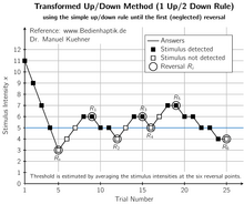
Diagram showing a specific staircase procedure: Transformed Up/Down Method (1 up/ 2 down rule). Until the first reversal (which is neglected) the simple up/down rule and a larger step size is used.

Staircases usually begin with a high intensity stimulus, which is easy to detect. The intensity is then reduced until the observer makes a mistake, at which point the staircase 'reverses' and intensity is increased until the observer responds correctly, triggering another reversal. The values for the last of these 'reversals' are then averaged. There are many different types of staircase procedures, using different decision and termination rules. Step-size, up/down rules and the spread of the underlying psychometric function dictate where on the psychometric function they converge.^[25] Threshold values obtained from staircases can fluctuate wildly, so care must be taken in their design. Many different staircase algorithms have been modeled and some practical recommendations suggested by Garcia-Perez.^[26]

One of the more common staircase designs (with fixed-step sizes) is the 1-up-N-down staircase. If the participant makes the correct response N times in a row, the stimulus intensity is reduced by one step size. If the participant makes an incorrect response the stimulus intensity is increased by the one size. A threshold is estimated from the mean midpoint of all runs. This estimate approaches, asymptotically, the correct threshold.

Bayesian and maximum-likelihood procedures

Bayesian and maximum-likelihood adaptive procedures behave, from the observer's perspective, similar to the staircase procedures. The choice of the next intensity level works differently, however: After each observer response, from the set of this and all previous stimulus/response pairs the likelihood is calculated of where the threshold lies. The point of maximum likelihood is then chosen as the best estimate for the threshold, and the next stimulus is presented at that level (since a decision at that level will add the most information). In a Bayesian procedure, a prior likelihood is further included in the calculation.^[25] Compared to staircase procedures, Bayesian and ML procedures are more time-consuming to implement but are considered to be more robust. Well-known procedures of this kind are Quest,^[27] ML-PEST,^[28] and Kontsevich & Tyler’s method.^[29]

Magnitude estimation

In the prototypical case, people are asked to assign numbers in proportion to the magnitude of the stimulus. This psychometric function of the geometric means of their numbers is often a power law with stable, replicable exponent. Although contexts can change the law and exponent, that change too is stable and replicable. Instead of numbers, other sensory or cognitive dimensions can be used to match a stimulus and the method then becomes "magnitude production" or "cross-modality matching". The exponents of those dimensions found in numerical magnitude estimation predict the exponents found in magnitude production. Magnitude estimation generally finds lower exponents for the psychophysical function than multiple-category responses, because of the restricted range of the categorical anchors, such as those used by Likert as items in attitude scales.

Computer vision

From Wikipedia, the free encyclopedia

Computer vision is a field that deals with how computers can be made for gaining high-level understanding from digital images or videos. From the perspective of engineering, it seeks to automate tasks that a human can do.

Computer vision tasks include method for image processing, and understanding digital images, and extraction of high dimensional data from the real world in order to produce numerical or symbolic information, e.g., in the forms of decisions. Understanding in this context means the transformation of visual images (the input of the retina) into descriptions of the world that can interface with other thought processes and elicit appropriate action. This image understanding can be seen as the disentangling of symbolic information from image data using models constructed with the aid of geometry, physics, statistics, and learning theory.

As a computer vision is concerned with the theory behind artificial systems that extract information from images. The image data can take many forms, such as video sequences, views from multiple cameras, or multi-dimensional data from a medical scanner. As a technological discipline, computer vision seeks to apply its theories and models for the construction of computer vision systems.

Sub-domains of computer vision include scene reconstruction, event detection, learning, indexing, motion estimation.

Definition

Computer vision is an interdisciplinary field that deals with how computers can be made for gaining high-level understanding from digital images or videos. From the perspective of engineering, it seeks to automate tasks that the human visual system can do. Computer vision is concerned with the automatic extraction, analysis and understanding of useful information from a single image or a sequence of images. It involves the development of a theoretical and algorithmic basis to achieve automatic visual understanding. Computer vision is concerned with the theory behind artificial systems that extract information from images. The image data can take many forms, such as video sequences, views from multiple cameras, or multi-dimensional data from a medical scanner “tricorder” medical scanner.

History

In the late 1960s, computer vision began at universities that were pioneering artificial intelligence. It was meant to mimic the human visual system, as a stepping stone to endowing robots with intelligent behavior.^[1] In 1966, it was believed that this could be achieved through a summer project, by attaching a camera to a computer and having it "describe what it saw".^[2][3]

What distinguished computer vision from the prevalent field of digital image processing at that time was a desire to extract three-dimensional structure from images with the goal of achieving full scene understanding. Studies in the 1970s formed the early foundations for many of the computer vision algorithms that exist today, including extraction of edges from images, labeling of lines, non-polyhedral and polyhedral modeling, representation of objects as interconnections of smaller structures, optical flow, and motion estimation.^[1]

The next decade saw studies based on more rigorous mathematical analysis and quantitative aspects of computer vision. These include the concept of scale-space, the inference of shape from various cues such as shading, texture and focus, and contour models known as snakes. Researchers also realized that many of these mathematical concepts could be treated within the same optimization framework as regularization and Markov random fields.^[4] By the 1990s, some of the previous research topics became more active than the others. Research in projective 3-D reconstructions led to better understanding of camera calibration. With the advent of optimization methods for camera calibration, it was realized that a lot of the ideas were already explored in bundle adjustment theory from the field of photogrammetry. This led to methods for sparse 3-D reconstructions of scenes from multiple images. Progress was made on the dense stereo correspondence problem and further multi-view stereo techniques. At the same time, variations of graph cut were used to solve image segmentation. This decade also marked the first time statistical learning techniques were used in practice to recognize faces in images (see Eigenface). Toward the end of the 1990s, a significant change came about with the increased interaction between the fields of computer graphics and computer vision. This included image-based rendering, image morphing, view interpolation, panoramic image stitching and early light-field rendering.^[1]

Recent work has seen the resurgence of feature-based methods, used in conjunction with machine learning techniques and complex optimization frameworks.^[5][6]

Related fields

Areas of artificial intelligence deal with autonomous planning or deliberation for robotical systems to navigate through an environment. A detailed understanding of these environments is required to navigate through them. Information about the environment could be provided by a computer vision system, acting as a vision sensor and providing high-level information about the environment and the robot.

Artificial intelligence and computer vision share other topics such as pattern recognition and learning techniques. Consequently, computer vision is sometimes seen as a part of the artificial intelligence field or the computer science field in general.

Solid-state physics is another field that is closely related to computer vision. Most computer vision systems rely on image sensors, which detect electromagnetic radiation, which is typically in the form of either visible or infra-red light. The sensors are designed using quantum physics. The process by which light interacts with surfaces is explained using physics. Physics explains the behavior of optics which are a core part of most imaging systems. Sophisticated image sensors even require quantum mechanics to provide a complete understanding of the image formation process. Also, various measurement problems in physics can be addressed using computer vision, for example motion in fluids.

A third field which plays an important role is neurobiology, specifically the study of the biological vision system. Over the last century, there has been an extensive study of eyes, neurons, and the brain structures devoted to processing of visual stimuli in both humans and various animals. This has led to a coarse, yet complicated, description of how "real" vision systems operate in order to solve certain vision related tasks. These results have led to a subfield within computer vision where artificial systems are designed to mimic the processing and behavior of biological systems, at different levels of complexity. Also, some of the learning-based methods developed within computer vision (e.g. neural net and deep learning based image and feature analysis and classification) have their background in biology.

Some strands of computer vision research are closely related to the study of biological vision – indeed, just as many strands of AI research are closely tied with research into human consciousness, and the use of stored knowledge to interpret, integrate and utilize visual information. The field of biological vision studies and models the physiological processes behind visual perception in humans and other animals. Computer vision, on the other hand, studies and describes the processes implemented in software and hardware behind artificial vision systems. Interdisciplinary exchange between biological and computer vision has proven fruitful for both fields.

Yet another field related to computer vision is signal processing. Many methods for processing of one-variable signals, typically temporal signals, can be extended in a natural way to processing of two-variable signals or multi-variable signals in computer vision. However, because of the specific nature of images there are many methods developed within computer vision which have no counterpart in processing of one-variable signals. Together with the multi-dimensionality of the signal, this defines a subfield in signal processing as a part of computer vision.

Beside the above-mentioned views on computer vision, many of the related research topics can also be studied from a purely mathematical point of view. For example, many methods in computer vision are based on statistics, optimization or geometry. Finally, a significant part of the field is devoted to the implementation aspect of computer vision; how existing methods can be realized in various combinations of software and hardware, or how these methods can be modified in order to gain processing speed without losing too much performance.

The fields most closely related to computer vision are image processing, image analysis and machine vision. There is a significant overlap in the range of techniques and applications that these cover. This implies that the basic techniques that are used and developed in these fields are similar, something which can be interpreted as there is only one field with different names. On the other hand, it appears to be necessary for research groups, scientific journals, conferences and companies to present or market themselves as belonging specifically to one of these fields and, hence, various characterizations which distinguish each of the fields from the others have been presented.

Computer graphics produces image data from 3D models, computer vision often produces 3D models from image data ^[7]. There is also a trend towards a combination of the two disciplines, e.g., as explored in augmented reality.

The following characterizations appear relevant but should not be taken as universally accepted:

• Image processing and image analysis tend to focus on 2D images, how to transform one image to another, e.g., by pixel-wise operations such as contrast enhancement, local operations such as edge extraction or noise removal, or geometrical transformations such as rotating the image. This characterization implies that image processing/analysis neither require assumptions nor produce interpretations about the image content.
• Computer vision includes 3D analysis from 2D images. This analyzes the 3D scene projected onto one or several images, e.g., how to reconstruct structure or other information about the 3D scene from one or several images. Computer vision often relies on more or less complex assumptions about the scene depicted in an image.
• Machine vision is the process of applying a range of technologies & methods to provide imaging-based automatic inspection, process control and robot guidance^[8] in industrial applications.^[9] Machine vision tends to focus on applications, mainly in manufacturing, e.g., vision based robots and systems for vision based inspection, measurement, or picking (such as Bin Picking^[10]). This implies that image sensor technologies and control theory often are integrated with the processing of image data to control a robot and that real-time processing is emphasised by means of efficient implementations in hardware and software. It also implies that the external conditions such as lighting can be and are often more controlled in machine vision than they are in general computer vision, which can enable the use of different algorithms.
• There is also a field called imaging which primarily focus on the process of producing images, but sometimes also deals with processing and analysis of images. For example, medical imaging includes substantial work on the analysis of image data in medical applications.
• Finally, pattern recognition is a field which uses various methods to extract information from signals in general, mainly based on statistical approaches and artificial neural networks. A significant part of this field is devoted to applying these methods to image data.

Photogrammetry also overlaps with computer vision, e.g., stereophotogrammetry vs. computer stereo vision.

Applications

Applications range from tasks such as industrial machine vision systems which, say, inspect bottles speeding by on a production line, to research into artificial intelligence and computers or robots that can comprehend the world around them. The computer vision and machine vision fields have significant overlap. Computer vision covers the core technology of automated image analysis which is used in many fields. Machine vision usually refers to a process of combining automated image analysis with other methods and technologies to provide automated inspection and robot guidance in industrial applications. In many computer vision applications, the computers are pre-programmed to solve a particular task, but methods based on learning are now becoming increasingly common. Examples of applications of computer vision include systems for:

Learning 3D shapes has been a challenging task in computer vision. Recent advances in deep learning has enabled researchers to build models that are able to generate and reconstruct 3D shapes from single or multi-view depth maps or silhouettes seamlessly and efficiently ^[7]

• Automatic inspection, e.g., in manufacturing applications;
• Assisting humans in identification tasks, e.g., a species identification system;^[11]
• Controlling processes, e.g., an industrial robot;
• Detecting events, e.g., for visual surveillance or people counting;
• Interaction, e.g., as the input to a device for computer-human interaction;
• Modeling objects or environments, e.g., medical image analysis or topographical modeling;
• Navigation, e.g., by an autonomous vehicle or mobile robot; and
• Organizing information, e.g., for indexing databases of images and image sequences.

Play media

DARPA's Visual Media Reasoning concept video

One of the most prominent application fields is medical computer vision or medical image processing. This area is characterized by the extraction of information from image data for the purpose of making a medical diagnosis of a patient. Generally, image data is in the form of microscopy images, X-ray images, angiography images, ultrasonic images, and tomography images. An example of information which can be extracted from such image data is detection of tumours, arteriosclerosis or other malign changes. It can also be measurements of organ dimensions, blood flow, etc. This application area also supports medical research by providing new information, e.g., about the structure of the brain, or about the quality of medical treatments. Applications of computer vision in the medical area also includes enhancement of images that are interpreted by humans, for example ultrasonic images or X-ray images, to reduce the influence of noise.

A second application area in computer vision is in industry, sometimes called machine vision, where information is extracted for the purpose of supporting a manufacturing process. One example is quality control where details or final products are being automatically inspected in order to find defects. Another example is measurement of position and orientation of details to be picked up by a robot arm. Machine vision is also heavily used in agricultural process to remove undesirable food stuff from bulk material, a process called optical sorting.

Military applications are probably one of the largest areas for computer vision. The obvious examples are detection of enemy soldiers or vehicles and missile guidance. More advanced systems for missile guidance send the missile to an area rather than a specific target, and target selection is made when the missile reaches the area based on locally acquired image data. Modern military concepts, such as "battlefield awareness", imply that various sensors, including image sensors, provide a rich set of information about a combat scene which can be used to support strategic decisions. In this case, automatic processing of the data is used to reduce complexity and to fuse information from multiple sensors to increase reliability.

Artist's concept of a Mars Exploration Rover, an example of an unmanned land-based vehicle. Notice the stereo cameras mounted on top of the rover.

One of the newer application areas is autonomous vehicles, which include submersibles, land-based vehicles (small robots with wheels, cars or trucks), aerial vehicles, and unmanned aerial vehicles (UAV). The level of autonomy ranges from fully autonomous (unmanned) vehicles to vehicles where computer vision based systems support a driver or a pilot in various situations. Fully autonomous vehicles typically use computer vision for navigation, i.e. for knowing where it is, or for producing a map of its environment (SLAM) and for detecting obstacles. It can also be used for detecting certain task specific events, e.g., a UAV looking for forest fires. Examples of supporting systems are obstacle warning systems in cars, and systems for autonomous landing of aircraft. Several car manufacturers have demonstrated systems for autonomous driving of cars, but this technology has still not reached a level where it can be put on the market. There are ample examples of military autonomous vehicles ranging from advanced missiles, to UAVs for recon missions or missile guidance. Space exploration is already being made with autonomous vehicles using computer vision, e.g., NASA's Mars Exploration Rover and ESA's ExoMars Rover.

Other application areas include:

• Support of visual effects creation for cinema and broadcast, e.g., camera tracking (matchmoving).
• Surveillance.
• Tracking and counting organisms in the biological sciences ^[12]

Typical tasks

Each of the application areas described above employ a range of computer vision tasks; more or less well-defined measurement problems or processing problems, which can be solved using a variety of methods. Some examples of typical computer vision tasks are presented below.

Computer vision tasks include methods for acquiring, processing, analyzing and understanding digital images, and extraction of high-dimensional data from the real world in order to produce numerical or symbolic information, e.g., in the forms of decisions.^{[13][14][15][16]} Understanding in this context means the transformation of visual images (the input of the retina) into descriptions of the world that can interface with other thought processes and elicit appropriate action. This image understanding can be seen as the disentangling of symbolic information from image data using models constructed with the aid of geometry, physics, statistics, and learning theory.^[17]

Recognition

The classical problem in computer vision, image processing, and machine vision is that of determining whether or not the image data contains some specific object, feature, or activity.

Different varieties of the recognition problem are described in the literature:^{[citation needed]}

• Object recognition (also called object classification) – one or several pre-specified or learned objects or object classes can be recognized, usually together with their 2D positions in the image or 3D poses in the scene. Blippar, Google Goggles and LikeThat provide stand-alone programs that illustrate this functionality.
• Identification – an individual instance of an object is recognized. Examples include identification of a specific person's face or fingerprint, identification of handwritten digits, or identification of a specific vehicle.
• Detection – the image data are scanned for a specific condition. Examples include detection of possible abnormal cells or tissues in medical images or detection of a vehicle in an automatic road toll system. Detection based on relatively simple and fast computations is sometimes used for finding smaller regions of interesting image data which can be further analyzed by more computationally demanding techniques to produce a correct interpretation.

Currently, the best algorithms for such tasks are based on convolutional neural networks. An illustration of their capabilities is given by the ImageNet Large Scale Visual Recognition Challenge; this is a benchmark in object classification and detection, with millions of images and hundreds of object classes. Performance of convolutional neural networks, on the ImageNet tests, is now close to that of humans.^[18] The best algorithms still struggle with objects that are small or thin, such as a small ant on a stem of a flower or a person holding a quill in their hand. They also have trouble with images that have been distorted with filters (an increasingly common phenomenon with modern digital cameras). By contrast, those kinds of images rarely trouble humans. Humans, however, tend to have trouble with other issues. For example, they are not good at classifying objects into fine-grained classes, such as the particular breed of dog or species of bird, whereas convolutional neural networks handle this with ease.

Several specialized tasks based on recognition exist, such as:

• Content-based image retrieval – finding all images in a larger set of images which have a specific content. The content can be specified in different ways, for example in terms of similarity relative a target image (give me all images similar to image X), or in terms of high-level search criteria given as text input (give me all images which contains many houses, are taken during winter, and have no cars in them).

Computer vision for people counter purposes in public places, malls, shopping centres

• Pose estimation – estimating the position or orientation of a specific object relative to the camera. An example application for this technique would be assisting a robot arm in retrieving objects from a conveyor belt in an assembly line situation or picking parts from a bin.
• Optical character recognition (OCR) – identifying characters in images of printed or handwritten text, usually with a view to encoding the text in a format more amenable to editing or indexing (e.g. ASCII).
• 2D Code reading Reading of 2D codes such as data matrix and QR codes.
• Facial recognition
• Shape Recognition Technology (SRT) in people counter systems differentiating human beings (head and shoulder patterns) from objects

Motion analysis

Several tasks relate to motion estimation where an image sequence is processed to produce an estimate of the velocity either at each points in the image or in the 3D scene, or even of the camera that produces the images . Examples of such tasks are:

• Egomotion – determining the 3D rigid motion (rotation and translation) of the camera from an image sequence produced by the camera.
• Tracking – following the movements of a (usually) smaller set of interest points or objects (e.g., vehicles, humans or other organisms ^[12]) in the image sequence.
• Optical flow – to determine, for each point in the image, how that point is moving relative to the image plane, i.e., its apparent motion. This motion is a result both of how the corresponding 3D point is moving in the scene and how the camera is moving relative to the scene.

Scene reconstruction

Given one or (typically) more images of a scene, or a video, scene reconstruction aims at computing a 3D model of the scene. In the simplest case the model can be a set of 3D points. More sophisticated methods produce a complete 3D surface model. The advent of 3D imaging not requiring motion or scanning, and related processing algorithms is enabling rapid advances in this field. Grid-based 3D sensing can be used to acquire 3D images from multiple angles. Algorithms are now available to stitch multiple 3D images together into point clouds and 3D models ^[7].

Image restoration

The aim of image restoration is the removal of noise (sensor noise, motion blur, etc.) from images. The simplest possible approach for noise removal is various types of filters such as low-pass filters or median filters. More sophisticated methods assume a model of how the local image structures look like, a model which distinguishes them from the noise. By first analysing the image data in terms of the local image structures, such as lines or edges, and then controlling the filtering based on local information from the analysis step, a better level of noise removal is usually obtained compared to the simpler approaches.

An example in this field is inpainting.

System methods

The organization of a computer vision system is highly application dependent. Some systems are stand-alone applications which solve a specific measurement or detection problem, while others constitute a sub-system of a larger design which, for example, also contains sub-systems for control of mechanical actuators, planning, information databases, man-machine interfaces, etc. The specific implementation of a computer vision system also depends on if its functionality is pre-specified or if some part of it can be learned or modified during operation. Many functions are unique to the application. There are, however, typical functions which are found in many computer vision systems.

• Image acquisition – A digital image is produced by one or several image sensors, which, besides various types of light-sensitive cameras, include range sensors, tomography devices, radar, ultra-sonic cameras, etc. Depending on the type of sensor, the resulting image data is an ordinary 2D image, a 3D volume, or an image sequence. The pixel values typically correspond to light intensity in one or several spectral bands (gray images or colour images), but can also be related to various physical measures, such as depth, absorption or reflectance of sonic or electromagnetic waves, or nuclear magnetic resonance.^[19]
• Pre-processing – Before a computer vision method can be applied to image data in order to extract some specific piece of information, it is usually necessary to process the data in order to assure that it satisfies certain assumptions implied by the method. Examples are
  • Re-sampling in order to assure that the image coordinate system is correct.
  • Noise reduction in order to assure that sensor noise does not introduce false information.
  • Contrast enhancement to assure that relevant information can be detected.
  • Scale space representation to enhance image structures at locally appropriate scales.
• Feature extraction – Image features at various levels of complexity are extracted from the image data.^[19] Typical examples of such features are
  • Lines, edges and ridges.
  • Localized interest points such as corners, blobs or points.

More complex features may be related to texture, shape or motion.

• Detection/segmentation – At some point in the processing a decision is made about which image points or regions of the image are relevant for further processing.^[19] Examples are
  • Selection of a specific set of interest points
  • Segmentation of one or multiple image regions which contain a specific object of interest.
  • Segmentation of image into nested scene architecture comprised foreground, object groups, single objects or salient object parts (also referred to as spatial-taxon scene hierarchy)^[20]
• High-level processing – At this step the input is typically a small set of data, for example a set of points or an image region which is assumed to contain a specific object.^[19] The remaining processing deals with, for example:
  • Verification that the data satisfy model-based and application specific assumptions.
  • Estimation of application specific parameters, such as object pose or object size.
  • Image recognition – classifying a detected object into different categories.
  • Image registration – comparing and combining two different views of the same object.
• Decision making Making the final decision required for the application,^[19] for example:
  • Pass/fail on automatic inspection applications
  • Match / no-match in recognition applications
  • Flag for further human review in medical, military, security and recognition applications

Image-understanding systems

Image-understanding systems (IUS) include three levels of abstraction as follows: Low level includes image primitives such as edges, texture elements, or regions; intermediate level includes boundaries, surfaces and volumes; and high level includes objects, scenes, or events. Many of these requirements are really topics for further research.

The representational requirements in the designing of IUS for these levels are: representation of prototypical concepts, concept organization, spatial knowledge, temporal knowledge, scaling, and description by comparison and differentiation.

While inference refers to the process of deriving new, not explicitly represented facts from currently known facts, control refers to the process that selects which of the many inference, search, and matching techniques should be applied at a particular stage of processing. Inference and control requirements for IUS are: search and hypothesis activation, matching and hypothesis testing, generation and use of expectations, change and focus of attention, certainty and strength of belief, inference and goal satisfaction.^[21]

Hardware

There are many kinds of computer vision systems, nevertheless all of them contain these basic elements: a power source, at least one image acquisition device (i.e. camera, ccd, etc.), a processor as well as control and communication cables or some kind of wireless interconnection mechanism. In addition, a practical vision system contains software, as well as a display in order to monitor the system. Vision systems for inner spaces, as most industrial ones, contain an illumination system and may be placed in a controlled environment. Furthermore, a completed system includes many accessories like camera supports, cables and connectors.

Most computer vision systems use visible-light cameras passively viewing a scene at frame rates of at most 60 frames per second (usually far slower).

A few computer vision systems use image acquisition hardware with active illumination or something other than visible light or both. For example, a structured-light 3D scanner, a thermographic camera, a hyperspectral imager, radar imaging, a lidar scanner, a magnetic resonance image, a side-scan sonar, a synthetic aperture sonar, or etc. Such hardware captures "images" that are then processed often using the same computer vision algorithms used to process visible-light images.

While traditional broadcast and consumer video systems operate at a rate of 30 frames per second, advances in digital signal processing and consumer graphics hardware has made high-speed image acquisition, processing, and display possible for real-time systems on the order of hundreds to thousands of frames per second. For applications in robotics, fast, real-time video systems are critically important and often can simplify the processing needed for certain algorithms. When combined with a high-speed projector, fast image acquisition allows 3D measurement and feature tracking to be realised.^[22]

Egocentric vision systems are composed of a wearable camera that automatically take pictures from a first-person perspective.

As of 2016, vision processing units are emerging as a new class of processor, to complement CPUs and graphics processing units (GPUs) in this role.^[23]