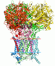
Structural bioinformatics

From Wikipedia, the free encyclopedia

https://en.wikipedia.org/wiki/Structural_bioinformatics 

Three-dimensional structure of a protein

Structural bioinformatics is the branch of bioinformatics that is related to the analysis and prediction of the three-dimensional structure of biological macromolecules such as proteins, RNA, and DNA. It deals with generalizations about macromolecular 3D structures such as comparisons of overall folds and local motifs, principles of molecular folding, evolution, binding interactions, and structure/function relationships, working both from experimentally solved structures and from computational models. The term structural has the same meaning as in structural biology, and structural bioinformatics can be seen as a part of computational structural biology. The main objective of structural bioinformatics is the creation of new methods of analysing and manipulating biological macromolecular data in order to solve problems in biology and generate new knowledge.

Introduction

Protein structure

Main article: Protein structure

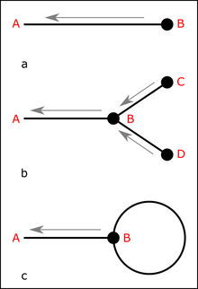
The structure of a protein is directly related to its function. The presence of certain chemical groups in specific locations allows proteins to act as enzymes, catalyzing several chemical reactions. In general, protein structures are classified into four levels: primary (sequences), secondary (local conformation of the polypeptide chain), tertiary (three-dimensional structure of the protein fold), and quaternary (association of multiple polypeptide structures). Structural bioinformatics mainly addresses interactions among structures taking into consideration their space coordinates. Thus, the primary structure is better analyzed in traditional branches of bioinformatics. However, the sequence implies restrictions that allow the formation of conserved local conformations of the polypeptide chain, such as alpha-helix, beta-sheets, and loops (secondary structure). Also, weak interactions (such as hydrogen bonds) stabilize the protein fold. Interactions could be intrachain, i.e., when occurring between parts of the same protein monomer (tertiary structure), or interchain, i.e., when occurring between different structures (quaternary structure). Finally, the topological arrangement of interactions, whether strong or weak, and entanglements is being studied in the field of structural bioinformatics, utilizing frameworks such as circuit topology.

Structure visualization

Structural visualization of BACTERIOPHAGE T4 LYSOZYME (PDB ID: 2LZM). (A) Cartoon; (B) Lines; (C) Surface; (D) Sticks.

Protein structure visualization is an important issue for structural bioinformatics. It allows users to observe static or dynamic representations of the molecules, also allowing the detection of interactions that may be used to make inferences about molecular mechanisms. The most common types of visualization are:

• Cartoon: this type of protein visualization highlights the secondary structure differences. In general, α-helix is represented as a type of screw, β-strands as arrows, and loops as lines.
• Lines: each amino acid residue is represented by thin lines, which allows a low cost for graphic rendering.
• Surface: in this visualization, the external shape of the molecule is shown.
• Sticks: each covalent bond between amino acid atoms is represented as a stick. This type of visualization is most used to visualize interactions between amino acids...

DNA structure

The classic DNA duplexes structure was initially described by Watson and Crick (and contributions of Rosalind Franklin). The DNA molecule is composed of three substances: a phosphate group, a pentose, and a nitrogen base (adenine, thymine, cytosine, or guanine). The DNA double helix structure is stabilized by hydrogen bonds formed between base pairs: adenine with thymine (A-T) and cytosine with guanine (C-G). Many structural bioinformatics studies have focused on understanding interactions between DNA and small molecules, which has been the target of several drug design studies.

Interactions

Interactions are contacts established between parts of molecules at different levels. They are responsible for stabilizing protein structures and perform a varied range of activities. In biochemistry, interactions are characterized by the proximity of atom groups or molecules regions that present an effect upon one another, such as electrostatic forces, hydrogen bonding, and hydrophobic effect. Proteins can perform several types of interactions, such as protein-protein interactions (PPI), protein-peptide interactions, protein-ligand interactions (PLI), and protein-DNA interaction.

Contacts between two amino acid residues: Q196-R200 (PDB ID- 2X1C) 

Calculating contacts

Calculating contacts is an important task in structural bioinformatics, being important for the correct prediction of protein structure and folding, thermodynamic stability, protein-protein and protein-ligand interactions, docking and molecular dynamics analyses, and so on.

Traditionally, computational methods have used threshold distance between atoms (also called cutoff) to detect possible interactions. This detection is performed based on Euclidean distance and angles between atoms of determined types. However, most of the methods based on simple Euclidean distance cannot detect occluded contacts. Hence, cutoff free methods, such as Delaunay triangulation, have gained prominence in recent years. In addition, the combination of a set of criteria, for example, physicochemical properties, distance, geometry, and angles, have been used to improve the contact determination.

Protein Data Bank (PDB)

Main article: Protein Data Bank

The number of structures from PDB. (A) The overall growth of released structures in Protein DataBank per year. (B) Growth of structures deposited in PDB from X-ray crystallography, NMR spectroscopy, and 3D electron microscopy experiments per year. Source: https://www.rcsb.org/stats/growth

The Protein Data Bank (PDB) is a database of 3D structure data for large biological molecules, such as proteins, DNA, and RNA. PDB is managed by an international organization called the Worldwide Protein Data Bank (wwPDB), which is composed of several local organizations, as. PDBe, PDBj, RCSB, and BMRB. They are responsible for keeping copies of PDB data available on the internet at no charge. The number of structure data available at PDB has increased each year, being obtained typically by X-ray crystallography, NMR spectroscopy, or cryo-electron microscopy.

Data format

The PDB format (.pdb) is the legacy textual file format used to store information of three-dimensional structures of macromolecules used by the Protein Data Bank. Due to restrictions in the format structure conception, the PDB format does not allow large structures containing more than 62 chains or 99999 atom records.

The PDBx/mmCIF (macromolecular Crystallographic Information File) is a standard text file format for representing crystallographic information. Since 2014, the PDB format was substituted as the standard PDB archive distribution by the PDBx/mmCIF file format (.cif). While PDB format contains a set of records identified by a keyword of up to six characters, the PDBx/mmCIF format uses a structure based on key and value, where the key is a name that identifies some feature and the value is the variable information.

Other structural databases

In addition to the Protein Data Bank (PDB), there are several databases of protein structures and other macromolecules. Examples include:

• MMDB: Experimentally determined three-dimensional structures of biomolecules derived from Protein Data Bank (PDB).
• Nucleic acid Data Base (NDB): Experimentally determined information about nucleic acids (DNA, RNA).
• Structural Classification of Proteins (SCOP): Comprehensive description of the structural and evolutionary relationships between structurally known proteins.
• TOPOFIT-DB: Protein structural alignments based on the TOPOFIT method.
• Electron Density Server (EDS): Electron-density maps and statistics about the fit of crystal structures and their maps.
• CASP: Prediction Center Community-wide, worldwide experiment for protein structure prediction CASP.
• PISCES server for creating non-redundant lists of proteins: Generates PDB list by sequence identity and structural quality criteria.
• The Structural Biology Knowledgebase: Tools to aid in protein research design.
• ProtCID: The Protein Common Interface Database Database of similar protein-protein interfaces in crystal structures of homologous proteins.
• AlphaFold:AlphaFold - Protein Structure Database.

Structure comparison

Structural alignment

Structural alignment is a method for comparison between 3D structures based on their shape and conformation. It could be used to infer the evolutionary relationship among a set of proteins even with low sequence similarity. Structural alignment implies superimposing a 3D structure over a second one, rotating and translating atoms in corresponding positions (in general, using the C_α atoms or even the backbone heavy atoms C, N, O, and C_α). Usually, the alignment quality is evaluated based on the root-mean-square deviation (RMSD) of atomic positions, i.e., the average distance between atoms after superimposition:

${\displaystyle \mathrm{R}\mathrm{M}\mathrm{S}\mathrm{D}=\sqrt{\frac{1}{N}\sum _{i=1}^N{\delta }_i^2}}$

where δ_i is the distance between atom i and either a reference atom corresponding in the other structure or the mean coordinate of the N equivalent atoms. In general, the RMSD outcome is measured in Ångström (Å) unit, which is equivalent to 10⁻¹⁰ m. The nearer to zero the RMSD value, the more similar are the structures.

Graph-based structural signatures

Structural signatures, also called fingerprints, are macromolecule pattern representations that can be used to infer similarities and differences. Comparisons among a large set of proteins using RMSD still is a challenge due to the high computational cost of structural alignments. Structural signatures based on graph distance patterns among atom pairs have been used to determine protein identifying vectors and to detect non-trivial information. Furthermore, linear algebra and machine learning can be used for clustering protein signatures, detecting protein-ligand interactions, predicting ΔΔG, and proposing mutations based on Euclidean distance.

Structure prediction

A Ramachandran plot generated from human PCNA (PDB ID 1AXC). The red, brown, and yellow regions represent the favored, allowed, and "generously allowed" regions as defined by ProCheck. This plot can be used to verify incorrectly modeled amino acids.

The atomic structures of molecules can be obtained by several methods, such as X-ray crystallography (XRC), NMR spectroscopy, and 3D electron microscopy; however, these processes can present high costs and sometimes some structures can be hardly established, such as membrane proteins. Hence, it is necessary to use computational approaches for determining 3D structures of macromolecules. The structure prediction methods are classified into comparative modeling and de novo modeling.

Comparative modeling

Comparative modeling, also known as homology modeling, corresponds to the methodology to construct three-dimensional structures from an amino acid sequence of a target protein and a template with known structure. The literature has described that evolutionarily related proteins tend to present a conserved three-dimensional structure. In addition, sequences of distantly related proteins with identity lower than 20% can present different folds.

De novo modeling

In structural bioinformatics, de novo modeling, also known as ab initio modeling, refers to approaches for obtaining three-dimensional structures from sequences without the necessity of a homologous known 3D structure. Despite the new algorithms and methods proposed in the last years, de novo protein structure prediction is still considered one of the remain outstanding issues in modern science.

Structure validation

After structure modeling, an additional step of structure validation is necessary since many of both comparative and 'de novo' modeling algorithms and tools use heuristics to try assembly the 3D structure, which can generate many errors. Some validation strategies consist of calculating energy scores and comparing them with experimentally determined structures. For example, the DOPE score is an energy score used by the MODELLER tool for determining the best model.

Another validation strategy is calculating φ and ψ backbone dihedral angles of all residues and construct a Ramachandran plot. The side-chain of amino acids and the nature of interactions in the backbone restrict these two angles, and thus, the visualization of allowed conformations could be performed based on the Ramachandran plot. A high quantity of amino acids allocated in no permissive positions of the chart is an indication of a low-quality modeling.

Prediction tools

A list with commonly used software tools for protein structure prediction, including comparative modeling, protein threading, de novo protein structure prediction, and secondary structure prediction is available in the list of protein structure prediction software.

Molecular docking

Representation of docking a ligand (green) to a protein target (black).

Molecular docking (also referred to only as docking) is a method used to predict the orientation coordinates of a molecule (ligand) when bound to another one (receptor or target). The binding may be mostly through non-covalent interactions while covalently linked binding can also be studied. Molecular docking aims to predict possible poses (binding modes) of the ligand when it interacts with specific regions on the receptor. Docking tools use force fields to estimate a score for ranking best poses that favored better interactions between the two molecules.

In general, docking protocols are used to predict the interactions between small molecules and proteins. However, docking also can be used to detect associations and binding modes among proteins, peptides, DNA or RNA molecules, carbohydrates, and other macromolecules.

Virtual screening

Virtual screening (VS) is a computational approach used for fast screening of large compound libraries for drug discovery. Usually, virtual screening uses docking algorithms to rank small molecules with the highest affinity to a target receptor.

In recent times, several tools have been used to evaluate the use of virtual screening in the process of discovering new drugs. However, problems such as missing information, inaccurate understanding of drug-like molecular properties, weak scoring functions, or insufficient docking strategies hinder the docking process. Hence, the literature has described that it is still not considered a mature technology.

Molecular dynamics

Example: molecular dynamics of a glucose-tolerant β-Glucosidase

Molecular dynamics (MD) is a computational method for simulating interactions between molecules and their atoms during a given period of time. This method allows the observation of the behavior of molecules and their interactions, considering the system as a whole. To calculate the behavior of the systems and, thus, determine the trajectories, an MD can use Newton's equation of motion, in addition to using molecular mechanics methods to estimate the forces that occur between particles (force fields).

Applications

Informatics approaches used in structural bioinformatics are:

• Selection of Target - Potential targets are identified by comparing them with databases of known structures and sequence. The importance of a target can be decided on the basis of published literature. Target can also be selected on the basis of its protein domain. Protein domains are building blocks that can be rearranged to form new proteins. They can be studied in isolation initially.
• Tracking X-ray crystallography trials - X-Ray crystallography can be used to reveal three-dimensional structure of a protein. But, in order to use X-ray for studying protein crystals, pure proteins crystals must be formed, which can take a lot of trials. This leads to a need for tracking the conditions and results of trials. Furthermore, supervised machine learning algorithms can be used on the stored data to identify conditions that might increase the yield of pure crystals.
• Analysis of X-Ray crystallographic data - The diffraction pattern obtained as a result of bombarding X-rays on electrons is Fourier transform of electron density distribution. There is a need for algorithms that can deconvolve Fourier transform with partial information ( due to missing phase information, as the detectors can only measure amplitude of diffracted X-rays, and not the phase shifts ). Extrapolation technique such as Multiwavelength anomalous dispersion can be used to generate electron density map, which uses the location of selenium atoms as a reference to determine rest of the structure. Standard Ball-and-stick model is generated from the electron density map.
• Analysis of NMR spectroscopy data - Nuclear magnetic resonance spectroscopy experiments produce two (or higher) dimensional data, with each peak corresponding to a chemical group within the sample. Optimization methods are used to convert spectra into three dimensional structures.
• Correlating Structural information with functional information - Structural studies can be used as probe for structural-functional relationship.

Tools

Distance criteria for contact definition

List of structural bioinformatics tools

Type	Max distance criteria
Hydrogen bond	3,9 Å
Hydrophobic interaction	5 Å
Ionic interaction	6 Å
Aromatic Stacking	6 Å
Software	Description
I-TASSER	Predicting three-dimensional structure model of protein molecules from amino acid sequences.
MOE	Molecular Operating Environment (MOE) is an extensive platform including structural modeling for proteins, protein families and antibodies
SBL	The Structural Bioinformatics Library: end-user applications and advanced algorithms
BALLView	Molecular modeling and visualization
STING	Visualization and analysis
PyMOL	Viewer and modeling
VMD	Viewer, molecular dynamics
KiNG	An open-source Java kinemage viewer
STRIDE	Determination of secondary structure from coordinates
DSSP	Algorithm assigning a secondary structure to the amino acids of a protein
MolProbity	Structure-validation web server
PROCHECK	A structure-validation web service
CheShift	A protein structure-validation on-line application
3D-mol.js	A molecular viewer for web applications developed using Javascript
PROPKA	Rapid prediction of protein pKa values based on empirical structure/function relationships
CARA	Computer Aided Resonance Assignment
Docking Server	A molecular docking web server
StarBiochem	A java protein viewer, features direct search of protein databank
SPADE	The structural proteomics application development environment
PocketSuite	A web portal for various web-servers for binding site-level analysis. PocketSuite is divided into:: PocketDepth (Binding site prediction) PocketMatch (Binding site comparison), PocketAlign (Binding site alignment), and PocketAnnotate (Binding site annotation).
MSL	An open-source C++ molecular modeling software library for the implementation of structural analysis, prediction and design methods
PSSpred	Protein secondary structure prediction
Proteus	Webtool for suggesting mutation pairs
SDM	A server for predicting effects of mutations on protein stability

Information field theory

From Wikipedia, the free encyclopedia

https://en.wikipedia.org/wiki/Information_field_theory 

Information field theory (IFT) is a Bayesian statistical field theory relating to signal reconstruction, cosmography, and other related areas. IFT summarizes the information available on a physical field using Bayesian probabilities. It uses computational techniques developed for quantum field theory and statistical field theory to handle the infinite number of degrees of freedom of a field and to derive algorithms for the calculation of field expectation values. For example, the posterior expectation value of a field generated by a known Gaussian process and measured by a linear device with known Gaussian noise statistics is given by a generalized Wiener filter applied to the measured data. IFT extends such known filter formula to situations with nonlinear physics, nonlinear devices, non-Gaussian field or noise statistics, dependence of the noise statistics on the field values, and partly unknown parameters of measurement. For this it uses Feynman diagrams, renormalisation flow equations, and other methods from mathematical physics.

Motivation

Fields play an important role in science, technology, and economy. They describe the spatial variations of a quantity, like the air temperature, as a function of position. Knowing the configuration of a field can be of large value. Measurements of fields, however, can never provide the precise field configuration with certainty. Physical fields have an infinite number of degrees of freedom, but the data generated by any measurement device is always finite, providing only a finite number of constraints on the field. Thus, an unambiguous deduction of such a field from measurement data alone is impossible and only probabilistic inference remains as a means to make statements about the field. Fortunately, physical fields exhibit correlations and often follow known physical laws. Such information is best fused into the field inference in order to overcome the mismatch of field degrees of freedom to measurement points. To handle this, an information theory for fields is needed, and that is what information field theory is.

Concepts

Bayesian inference

${\displaystyle s(x)}$ is a field value at a location ${\displaystyle x\in \mathrm{\Omega }}$ in a space ${\displaystyle \mathrm{\Omega }}$. The prior knowledge about the unknown signal field ${\displaystyle s}$ is encoded in the probability distribution ${\displaystyle \mathcal{P}(s)}$. The data ${\displaystyle d}$ provides additional information on ${\displaystyle s}$ via the likelihood ${\displaystyle \mathcal{P}(d|s)}$ that gets incorporated into the posterior probability

$${\displaystyle \mathcal{P}(s|d)=\frac{\mathcal{P}(d|s)\mathcal{P}(s)}{\mathcal{P}(d)}}$$

according to Bayes theorem.

Information Hamiltonian

In IFT Bayes theorem is usually rewritten in the language of a statistical field theory,

$${\displaystyle \mathcal{P}(s|d)=\frac{\mathcal{P}(d,s)}{\mathcal{P}(d)}\equiv \frac{e^{-\mathcal{H}(d,s)}}{\mathcal{Z}(d)},}$$

with the information Hamiltonian defined as

$${\displaystyle \mathcal{H}(d,s)\equiv -\ln \mathcal{P}(d,s)=-\ln \mathcal{P}(d|s)-\ln \mathcal{P}(s)\equiv \mathcal{H}(d|s)+\mathcal{H}(s),}$$

the negative logarithm of the joint probability of data and signal and with the partition function being

$${\displaystyle \mathcal{Z}(d)\equiv \mathcal{P}(d)=\int \mathcal{D}s\mathcal{P}(d,s).}$$

This reformulation of Bayes theorem permits the usage of methods of mathematical physics developed for the treatment of statistical field theories and quantum field theories.

Fields

As fields have an infinite number of degrees of freedom, the definition of probabilities over spaces of field configurations has subtleties. Identifying physical fields as elements of function spaces provides the problem that no Lebesgue measure is defined over the latter and therefore probability densities can not be defined there. However, physical fields have much more regularity than most elements of function spaces, as they are continuous and smooth at most of their locations. Therefore less general, but sufficiently flexible constructions can be used to handle the infinite number of degrees of freedom of a field.

A pragmatic approach is to regard the field to be discretized in terms of pixels. Each pixel carries a single field value that is assumed to be constant within the pixel volume. All statements about the continuous field have then to be cast into its pixel representation. This way, one deals with finite dimensional field spaces, over which probability densities are well definable.

In order for this description to be a proper field theory, it is further required that the pixel resolution ${\displaystyle \mathrm{\Delta }x}$ can always be refined, while expectation values of the discretized field ${\displaystyle s_{\mathrm{\Delta }x}}$ converge to finite values:

$${\displaystyle ⟨f(s){⟩}_{(s|d)}\equiv \underset{\mathrm{\Delta }x\to 0}{lim}\int d{s}_{\mathrm{\Delta }x}f(s_{\mathrm{\Delta }x})\mathcal{P}(s_{\mathrm{\Delta }x}).}$$

Path integrals

If this limit exists, one can talk about the field configuration space integral or path integral

$${\displaystyle ⟨f(s){⟩}_{(s|d)}\equiv \int \mathcal{D}sf(s)\mathcal{P}(s).}$$

irrespective of the resolution it might be evaluated numerically.

Gaussian prior

The simplest prior for a field is that of a zero mean Gaussian probability distribution

$${\displaystyle \mathcal{P}(s)=\mathcal{G}(s,S)\equiv \frac{1}{|2\pi S|}{e}^{-\frac{1}{2}{s}^{†}{S}^{-1}s}.}$$

The determinant in the denominator might be ill-defined in the continuum limit ${\displaystyle \mathrm{\Delta }x\to 0}$, however, all what is necessary for IFT to be consistent is that this determinant can be estimated for any finite resolution field representation with ${\displaystyle \mathrm{\Delta }x>0}$ and that this permits the calculation of convergent expectation values.

A Gaussian probability distribution requires the specification of the field two point correlation function ${\displaystyle S\equiv ⟨s{s}^{†}{⟩}_{(s)}}$ with coefficients

$${\displaystyle S_{xy}\equiv ⟨s(x)\overline{s(y)}{⟩}_{(s)}}$$

and a scalar product for continuous fields

$${\displaystyle a^{†}b\equiv {\int }_{\mathrm{\Omega }}dx\overline{a(x)}b(x),}$$

with respect to which the inverse signal field covariance ${\displaystyle S^{-1}}$ is constructed, i.e. ${\displaystyle (S^{-1}S{)}_{xy}\equiv {\int }_{\mathrm{\Omega }}dz(S^{-1}{)}_{xz}{S}_{zy}={\mathbb{1}}_{xy}\equiv \delta (x-y).}$

The corresponding prior information Hamiltonian reads

$${\displaystyle \mathcal{H}(s)=-\ln \mathcal{G}(s,S)=\frac{1}{2}{s}^{†}{S}^{-1}s+\frac{1}{2}\ln |2\pi S|.}$$

Measurement equation

The measurement data ${\displaystyle d}$ was generated with the likelihood ${\displaystyle \mathcal{P}(d|s)}$. In case the instrument was linear, a measurement equation of the form

$${\displaystyle d=Rs+n}$$

can be given, in which ${\displaystyle R}$ is the instrument response, which describes how the data on average reacts to the signal, and ${\displaystyle n}$ is the noise, simply the difference between data ${\displaystyle d}$ and linear signal response ${\displaystyle Rs}$. It is essential to note that the response translates the infinite dimensional signal vector into the finite dimensional data space. In components this reads ${\displaystyle d_i={\int }_{\mathrm{\Omega }}dx{R}_{ix}{s}_x+n_i,}$

where a vector component notation was also introduced for signal and data vectors.

If the noise follows a signal independent zero mean Gaussian statistics with covariance ${\displaystyle N}$, ${\displaystyle \mathcal{P}(n|s)=\mathcal{G}(n,N),}$ then the likelihood is Gaussian as well,

$${\displaystyle \mathcal{P}(d|s)=\mathcal{G}(d-Rs,N),}$$

and the likelihood information Hamiltonian is

$${\displaystyle \mathcal{H}(d|s)=-\ln \mathcal{G}(d-Rs,N)=\frac{1}{2}(d-Rs{)}^{†}{N}^{-1}(d-Rs)+\frac{1}{2}\ln |2\pi N|.}$$

A linear measurement of a Gaussian signal, subject to Gaussian and signal-independent noise leads to a free IFT.

Free theory

Free Hamiltonian

The joint information Hamiltonian of the Gaussian scenario described above is

$${\displaystyle \begin{array}{rl}\mathcal{H}(d,s)& =\mathcal{H}(d|s)+\mathcal{H}(s)\\ & \widehat{=}\frac{1}{2}(d-Rs{)}^{†}{N}^{-1}(d-Rs)+\frac{1}{2}{s}^{†}{S}^{-1}s\\ & \widehat{=}\frac{1}{2}\left[s^{†}\underset{D^{-1}}{\underbrace{(S^{-1}+R^{†}{N}^{-1}R)}}s-s^{†}\underset{j}{\underbrace{R^{†}{N}^{-1}d}}-\underset{j^{†}}{\underbrace{d^{†}{N}^{-1}R}}s\right]\\ & \equiv \frac{1}{2}\left[s^{†}{D}^{-1}s-s^{†}j-j^{†}s\right]\\ & =\frac{1}{2}\left[s^{†}{D}^{-1}s-s^{†}{D}^{-1}\underset{m}{\underbrace{Dj}}-\underset{m^{†}}{\underbrace{j^{†}D}}{D}^{-1}s\right]\\ & \widehat{=}\frac{1}{2}(s-m{)}^{†}{D}^{-1}(s-m),\end{array}}$$

where ${\displaystyle \widehat{=}}$ denotes equality up to irrelevant constants, which, in this case, means expressions that are independent of ${\displaystyle s}$. From this is it clear, that the posterior must be a Gaussian with mean ${\displaystyle m}$ and variance ${\displaystyle D}$,

$${\displaystyle \mathcal{P}(s|d)\propto e^{-\mathcal{H}(d,s)}\propto e^{-\frac{1}{2}(s-m{)}^{†}{D}^{-1}(s-m)}\propto \mathcal{G}(s-m,D)}$$

where equality between the right and left hand sides holds as both distributions are normalized, ${\displaystyle \int \mathcal{D}s\mathcal{P}(s|d)=1=\int \mathcal{D}s\mathcal{G}(s-m,D)}$.

Generalized Wiener filter

The posterior mean

$${\displaystyle m=Dj=(S^{-1}+R^{†}{N}^{-1}R{)}^{-1}{R}^{†}{N}^{-1}d}$$

is also known as the generalized Wiener filter solution and the uncertainty covariance

$${\displaystyle D=(S^{-1}+R^{†}{N}^{-1}R{)}^{-1}}$$

as the Wiener variance.

In IFT, ${\displaystyle j=R^{†}{N}^{-1}d}$ is called the information source, as it acts as a source term to excite the field (knowledge), and ${\displaystyle D}$ the information propagator, as it propagates information from one location to another in

$${\displaystyle m_x={\int }_{\mathrm{\Omega }}dy{D}_{xy}{j}_y.}$$

Interacting theory

Interacting Hamiltonian

If any of the assumptions that lead to the free theory is violated, IFT becomes an interacting theory, with terms that are of higher than quadratic order in the signal field. This happens when the signal or the noise are not following Gaussian statistics, when the response is non-linear, when the noise depends on the signal, or when response or covariances are uncertain.

In this case, the information Hamiltonian might be expandable in a Taylor-Fréchet series,

$${\displaystyle \mathcal{H}(d,s)=\underset{={\mathcal{H}}_{\text{free}}(d,s)}{\underbrace{\frac{1}{2}{s}^{†}{D}^{-1}s-j^{†}s+{\mathcal{H}}_0}}+\underset{={\mathcal{H}}_{\text{int}}(d,s)}{\underbrace{\sum _{n=3}^{\mathrm{\infty }}\frac{1}{n!}{\mathrm{\Lambda }}_{x_1...x_n}^{(n)}{s}_{x_1}...s_{x_n}}},}$$

where ${\displaystyle {\mathcal{H}}_{\text{free}}(d,s)}$ is the free Hamiltonian, which alone would lead to a Gaussian posterior, and ${\displaystyle {\mathcal{H}}_{\text{int}}(d,s)}$ is the interacting Hamiltonian, which encodes non-Gaussian corrections. The first and second order Taylor coefficients are often identified with the (negative) information source ${\displaystyle -j}$ and information propagator ${\displaystyle D}$, respectively. The higher coefficients ${\displaystyle {\mathrm{\Lambda }}_{x_1...x_n}^{(n)}}$are associated with non-linear self-interactions.

Classical field

The classical field ${\displaystyle s_{\text{cl}}}$ minimizes the information Hamiltonian,

$${\displaystyle {\frac{\mathrm{\partial }\mathcal{H}(d,s)}{\mathrm{\partial }s}|}_{s=s_{\text{cl}}}=0,}$$

and therefore maximizes the posterior:

$${\displaystyle {\frac{\mathrm{\partial }\mathcal{P}(s|d)}{\mathrm{\partial }s}|}_{s=s_{\text{cl}}}={\frac{\mathrm{\partial }}{\mathrm{\partial }s}\frac{e^{-\mathcal{H}(d,s)}}{\mathcal{Z}(d)}|}_{s=s_{\text{cl}}}=-\mathcal{P}(d,s)\underset{=0}{\underbrace{{\frac{\mathrm{\partial }\mathcal{H}(d,s)}{\mathrm{\partial }s}|}_{s=s_{\text{cl}}}}}=0}$$

The classical field ${\displaystyle s_{\text{cl}}}$ is therefore the maximum a posteriori estimator of the field inference problem.

Critical filter

The Wiener filter problem requires the two point correlation ${\displaystyle S\equiv ⟨s{s}^{†}{⟩}_{(s)}}$ of a field to be known. If it is unknown, it has to be inferred along with the field itself. This requires the specification of a hyperprior ${\displaystyle \mathcal{P}(S)}$. Often, statistical homogeneity (translation invariance) can be assumed, implying that ${\displaystyle S}$ is diagonal in Fourier space (for ${\displaystyle \mathrm{\Omega }={\mathbb{R}}^u}$ being a ${\displaystyle u}$ dimensional Cartesian space). In this case, only the Fourier space power spectrum ${\displaystyle P_s(\overrightarrow{k})}$ needs to be inferred. Given a further assumption of statistical isotropy, this spectrum depends only on the length ${\displaystyle k=|\overrightarrow{k}|}$ of the Fourier vector ${\displaystyle \overrightarrow{k}}$ and only a one dimensional spectrum ${\displaystyle P_s(k)}$ has to be determined. The prior field covariance reads then in Fourier space coordinates ${\displaystyle S_{\overrightarrow{k}\overrightarrow{q}}=(2\pi {)}^u\delta (\overrightarrow{k}-\overrightarrow{q})P_s(k)}$.

If the prior on ${\displaystyle P_s(k)}$ is flat, the joint probability of data and spectrum is

$${\displaystyle \begin{array}{rl}\mathcal{P}(d,P_s)& =\int \mathcal{D}s\mathcal{P}(d,s,P_s)\\ & =\int \mathcal{D}s\mathcal{P}(d|s,P_s)\mathcal{P}(s|P_s)\mathcal{P}(P_s)\\ & \propto \int \mathcal{D}s\mathcal{G}(d-Rs,N)\mathcal{G}(s,S)\\ & \propto \frac{1}{|S{|}^{\frac{1}{2}}}\int \mathcal{D}s\exp \left[-\frac{1}{2}\left(s^{†}{D}^{-1}s-j^{†}s-s^{†}j\right)\right]\\ & \propto \frac{|D{|}^{\frac{1}{2}}}{|S{|}^{\frac{1}{2}}}\exp \left[\frac{1}{2}{j}^{†}Dj\right],\end{array}}$$

where the notation of the information propagator ${\displaystyle D=(S^{-1}+R^{†}{N}^{-1}R{)}^{-1}}$ and source ${\displaystyle j=R^{†}{N}^{-1}d}$ of the Wiener filter problem was used again. The corresponding information Hamiltonian is

$${\displaystyle \mathcal{H}(d,P_s)\widehat{=}\frac{1}{2}\left[\ln |S{D}^{-1}|-j^{†}Dj\right]=\frac{1}{2}\mathrm{T}\mathrm{r}\left[\ln \left(S{D}^{-1}\right)-j{j}^{†}D\right],}$$

where ${\displaystyle \widehat{=}}$ denotes equality up to irrelevant constants (here: constant with respect to ${\displaystyle P_s}$). Minimizing this with respect to ${\displaystyle P_s}$, in order to get its maximum a posteriori power spectrum estimator, yields

$${\displaystyle \begin{array}{rl}\frac{\mathrm{\partial }\mathcal{H}(d,P_s)}{\mathrm{\partial }{P}_s(k)}& =\frac{1}{2}\mathrm{T}\mathrm{r}\left[D{S}^{-1}\frac{\mathrm{\partial }\left(S{D}^{-1}\right)}{\mathrm{\partial }{P}_s(k)}-j{j}^{†}\frac{\mathrm{\partial }D}{\mathrm{\partial }{P}_s(k)}\right]\\ & =\frac{1}{2}\mathrm{T}\mathrm{r}\left[D{S}^{-1}\frac{\mathrm{\partial }\left(1+S{R}^{†}{N}^{-1}R\right)}{\mathrm{\partial }{P}_s(k)}+j{j}^{†}D\frac{\mathrm{\partial }{D}^{-1}}{\mathrm{\partial }{P}_s(k)}D\right]\\ & =\frac{1}{2}\mathrm{T}\mathrm{r}\left[D{S}^{-1}\frac{\mathrm{\partial }S}{\mathrm{\partial }{P}_s(k)}{R}^{†}{N}^{-1}R+m{m}^{†}\frac{\mathrm{\partial }{S}^{-1}}{\mathrm{\partial }{P}_s(k)}\right]\\ & =\frac{1}{2}\mathrm{T}\mathrm{r}\left[\left(R^{†}{N}^{-1}RD{S}^{-1}-S^{-1}m{m}^{†}{S}^{-1}\right)\frac{\mathrm{\partial }S}{\mathrm{\partial }{P}_s(k)}\right]\\ & =\frac{1}{2}\int {\left(\frac{dq}{2\pi }\right)}^u\int {\left(\frac{d{q}^{\prime }}{2\pi }\right)}^u{\left(\left(D^{-1}-S^{-1}\right)D{S}^{-1}-S^{-1}m{m}^{†}{S}^{-1}\right)}_{\overrightarrow{q}{\overrightarrow{q}}^{\prime }}\frac{\mathrm{\partial }(2\pi {)}^u\delta (\overrightarrow{q}-{\overrightarrow{q}}^{\prime })P_s(q)}{\mathrm{\partial }{P}_s(k)}\\ & =\frac{1}{2}\int {\left(\frac{dq}{2\pi }\right)}^u{\left(S^{-1}-S^{-1}D{S}^{-1}-S^{-1}m{m}^{†}{S}^{-1}\right)}_{\overrightarrow{q}\overrightarrow{q}}\delta (k-q)\\ & =\frac{1}{2}\mathrm{T}\mathrm{r}\left\{S^{-1}\left[S-\left(D+m{m}^{†}\right)\right]S^{-1}{\mathbb{P}}_k\right\}\\ & =\frac{\mathrm{T}\mathrm{r}\left[{\mathbb{P}}_k\right]}{2P_s(k)}-\frac{\mathrm{T}\mathrm{r}\left[\left(D+m{m}^{†}\right){\mathbb{P}}_k\right]}{2{\left[P_s(k)\right]}^2}=0,\end{array}}$$

where the Wiener filter mean ${\displaystyle m=Dj}$ and the spectral band projector ${\displaystyle ({\mathbb{P}}_k{)}_{\overrightarrow{q}{\overrightarrow{q}}^{\prime }}\equiv (2\pi {)}^u\delta (\overrightarrow{q}-{\overrightarrow{q}}^{\prime })\delta (|\overrightarrow{q}|-k)}$were introduced. The latter commutes with ${\displaystyle S^{-1}}$, since ${\displaystyle (S^{-1}{)}_{\overrightarrow{k}\overrightarrow{q}}=(2\pi {)}^u\delta (\overrightarrow{k}-\overrightarrow{q})[P_s(k){]}^{-1}}$ is diagonal in Fourier space. The maximum a posteriori estimator for the power spectrum is therefore

$${\displaystyle P_s(k)=\frac{\mathrm{T}\mathrm{r}\left[\left(m{m}^{†}+D\right){\mathbb{P}}_k\right]}{\mathrm{T}\mathrm{r}\left[{\mathbb{P}}_k\right]}.}$$

It has to be calculated iteratively, as ${\displaystyle m=Dj}$ and ${\displaystyle D=(S^{-1}+R^{†}{N}^{-1}R{)}^{-1}}$ depend both on ${\displaystyle P_s}$ themselves. In an empirical Bayes approach, the estimated ${\displaystyle P_s}$ would be taken as given. As a consequence, the posterior mean estimate for the signal field is the corresponding ${\displaystyle m}$ and its uncertainty the corresponding ${\displaystyle D}$ in the empirical Bayes approximation.

The resulting non-linear filter is called the critical filter. The generalization of the power spectrum estimation formula as

$${\displaystyle P_s(k)=\frac{\mathrm{T}\mathrm{r}\left[\left(m{m}^{†}+\delta D\right){\mathbb{P}}_k\right]}{\mathrm{T}\mathrm{r}\left[{\mathbb{P}}_k\right]}}$$

exhibits a perception thresholds for ${\displaystyle \delta <1}$, meaning that the data variance in a Fourier band has to exceed the expected noise level by a certain threshold before the signal reconstruction ${\displaystyle m}$ becomes non-zero for this band. Whenever the data variance exceeds this threshold slightly, the signal reconstruction jumps to a finite excitation level, similar to a first order phase transition in thermodynamic systems. For filter with ${\displaystyle \delta =1}$ perception of the signal starts continuously as soon the data variance exceeds the noise level. The disappearance of the discontinuous perception at ${\displaystyle \delta =1}$ is similar to a thermodynamic system going through a critical point. Hence the name critical filter.

The critical filter, extensions thereof to non-linear measurements, and the inclusion of non-flat spectrum priors, permitted the application of IFT to real world signal inference problems, for which the signal covariance is usually unknown a priori.

IFT application examples

Radio interferometric image of radio galaxies in the galaxy cluster Abell 2219. The images were constructed by data back-projection (top), the CLEAN algorithm (middle), and the RESOLVE algorithm (bottom). Negative and therefore not physical fluxes are displayed in white.

The generalized Wiener filter, that emerges in free IFT, is in broad usage in signal processing. Algorithms explicitly based on IFT were derived for a number of applications. Many of them are implemented using the Numerical Information Field Theory (NIFTy) library.

• D³PO is a code for Denoising, Deconvolving, and Decomposing Photon Observations. It reconstructs images from individual photon count events taking into account the Poisson statistics of the counts and an instrument response function. It splits the sky emission into an image of diffuse emission and one of point sources, exploiting the different correlation structure and statistics of the two components for their separation. D³PO has been applied to data of the Fermi and the RXTE satellites.
• RESOLVE is a Bayesian algorithm for aperture synthesis imaging in radio astronomy. RESOLVE is similar to D³PO, but it assumes a Gaussian likelihood and a Fourier space response function. It has been applied to data of the Very Large Array.
• PySESA is a Python framework for Spatially Explicit Spectral Analysis for spatially explicit spectral analysis of point clouds and geospatial data.

Advanced theory

Many techniques from quantum field theory can be used to tackle IFT problems, like Feynman diagrams, effective actions, and the field operator formalism.

Feynman diagrams

First three Feynman diagrams contributing to the posterior mean estimate of a field. A line expresses an information propagator, a dot at the end of a line to an information source, and a vertex to an interaction term. The first diagram encodes the Wiener filter, the second a non-linear correction, and the third an uncertainty correction to the Wiener filter.

In case the interaction coefficients ${\displaystyle {\mathrm{\Lambda }}^{(n)}}$ in a Taylor-Fréchet expansion of the information Hamiltonian

$${\displaystyle \mathcal{H}(d,s)=\underset{={\mathcal{H}}_{\text{free}}(d,s)}{\underbrace{\frac{1}{2}{s}^{†}{D}^{-1}s-j^{†}s+{\mathcal{H}}_0}}+\underset{={\mathcal{H}}_{\text{int}}(d,s)}{\underbrace{\sum _{n=3}^{\mathrm{\infty }}\frac{1}{n!}{\mathrm{\Lambda }}_{x_1...x_n}^{(n)}{s}_{x_1}...s_{x_n}}},}$$

are small, the log partition function, or Helmholtz free energy,

$${\displaystyle \ln \mathcal{Z}(d)=\ln \int \mathcal{D}s{e}^{-\mathcal{H}(d,s)}=\sum _{c\in C}c}$$

can be expanded asymptotically in terms of these coefficients. The free Hamiltonian specifies the mean ${\displaystyle m=Dj}$ and variance ${\displaystyle D}$ of the Gaussian distribution ${\displaystyle \mathcal{G}(s-m,D)}$ over which the expansion is integrated. This leads to a sum over the set ${\displaystyle C}$ of all connected Feynman diagrams. From the Helmholtz free energy, any connected moment of the field can be calculated via

$${\displaystyle ⟨s_{x_1}\dots s_{x_n}{⟩}_{(s|d)}^{\text{c}}=\frac{{\mathrm{\partial }}^n\ln \mathcal{Z}}{\mathrm{\partial }{j}_{x_1}\dots \mathrm{\partial }{j}_{x_n}}.}$$

Situations where small expansion parameters exist that are needed for such a diagrammatic expansion to converge are given by nearly Gaussian signal fields, where the non-Gaussianity of the field statistics leads to small interaction coefficients ${\displaystyle {\mathrm{\Lambda }}^{(n)}}$. For example, the statistics of the Cosmic Microwave Background is nearly Gaussian, with small amounts of non-Gaussianities believed to be seeded during the inflationary epoch in the Early Universe.

Effective action

In order to have a stable numerics for IFT problems, a field functional that if minimized provides the posterior mean field is needed. Such is given by the effective action or Gibbs free energy of a field. The Gibbs free energy ${\displaystyle G}$ can be constructed from the Helmholtz free energy via a Legendre transformation. In IFT, it is given by the difference of the internal information energy

$${\displaystyle U=⟨\mathcal{H}(d,s){⟩}_{{\mathcal{P}}^{\prime }(s|d^{\prime })}}$$

and the Shannon entropy

$${\displaystyle \mathcal{S}=-\int \mathcal{D}s{\mathcal{P}}^{\prime }(s|d^{\prime })\ln {\mathcal{P}}^{\prime }(s|d^{\prime })}$$

for temperature ${\displaystyle T=1}$, where a Gaussian posterior approximation ${\displaystyle {\mathcal{P}}^{\prime }(s|d^{\prime })=\mathcal{G}(s-m,D)}$ is used with the approximate data ${\displaystyle d^{\prime }=(m,D)}$ containing the mean and the dispersion of the field.

The Gibbs free energy is then

$${\displaystyle \begin{array}{rl}G(m,D)& =U(m,D)-T\mathcal{S}(m,D)\\ & =⟨\mathcal{H}(d,s)+\ln {\mathcal{P}}^{\prime }(s|d^{\prime }){⟩}_{{\mathcal{P}}^{\prime }(s|d^{\prime })}\\ & =\int \mathcal{D}s{\mathcal{P}}^{\prime }(s|d^{\prime })\ln \frac{{\mathcal{P}}^{\prime }(s|d^{\prime })}{\mathcal{P}(d,s)}\\ & =\int \mathcal{D}s{\mathcal{P}}^{\prime }(s|d^{\prime })\ln \frac{{\mathcal{P}}^{\prime }(s|d^{\prime })}{\mathcal{P}(s|d)\mathcal{P}(d)}\\ & =\int \mathcal{D}s{\mathcal{P}}^{\prime }(s|d^{\prime })\ln \frac{{\mathcal{P}}^{\prime }(s|d^{\prime })}{\mathcal{P}(s|d)}-\ln \mathcal{P}(d)\\ & =\text{KL}({\mathcal{P}}^{\prime }(s|d^{\prime })||\mathcal{P}(s|d))-\ln \mathcal{Z}(d),\end{array}}$$

the Kullback-Leibler divergence ${\displaystyle \text{KL}({\mathcal{P}}^{\prime },\mathcal{P})}$ between approximative and exact posterior plus the Helmholtz free energy. As the latter does not depend on the approximate data ${\displaystyle d^{\prime }=(m,D)}$, minimizing the Gibbs free energy is equivalent to minimizing the Kullback-Leibler divergence between approximate and exact posterior. Thus, the effective action approach of IFT is equivalent to the variational Bayesian methods, which also minimize the Kullback-Leibler divergence between approximate and exact posteriors.

Minimizing the Gibbs free energy provides approximatively the posterior mean field

$${\displaystyle ⟨s{⟩}_{(s|d)}=\int \mathcal{D}ss\mathcal{P}(s|d),}$$

whereas minimizing the information Hamiltonian provides the maximum a posteriori field. As the latter is known to over-fit noise, the former is usually a better field estimator.

Operator formalism

The calculation of the Gibbs free energy requires the calculation of Gaussian integrals over an information Hamiltonian, since the internal information energy is

$${\displaystyle U(m,D)=⟨\mathcal{H}(d,s){⟩}_{{\mathcal{P}}^{\prime }(s|d^{\prime })}=\int \mathcal{D}s\mathcal{H}(d,s)\mathcal{G}(s-m,D).}$$

Such integrals can be calculated via a field operator formalism, in which

$${\displaystyle O_m=m+D\frac{\mathrm{d}}{\mathrm{d}m}}$$

is the field operator. This generates the field expression ${\displaystyle s}$ within the integral if applied to the Gaussian distribution function,

$${\displaystyle \begin{array}{rl}{O}_m\mathcal{G}(s-m,D)& =(m+D\frac{\mathrm{d}}{\mathrm{d}m})\frac{1}{|2\pi D{|}^{\frac{1}{2}}}\exp \left[-\frac{1}{2}(s-m{)}^{†}{D}^{-1}(s-m)\right]\\ & =(m+D{D}^{-1}(s-m))\frac{1}{|2\pi D{|}^{\frac{1}{2}}}\exp \left[-\frac{1}{2}(s-m{)}^{†}{D}^{-1}(s-m)\right]\\ & =s\mathcal{G}(s-m,D),\end{array}}$$

and any higher power of the field if applied several times,

$${\displaystyle \begin{array}{rl}(O_m{)}^n\mathcal{G}(s-m,D)& =s^n\mathcal{G}(s-m,D).\end{array}}$$

If the information Hamiltonian is analytical, all its terms can be generated via the field operator

$${\displaystyle \mathcal{H}(d,O_m)\mathcal{G}(s-m,D)=\mathcal{H}(d,s)\mathcal{G}(s-m,D).}$$

As the field operator does not depend on the field ${\displaystyle s}$ itself, it can be pulled out of the path integral of the internal information energy construction,

$${\displaystyle U(m,D)=\int \mathcal{D}s\mathcal{H}(d,O_m)\mathcal{G}(s-m,D)=\mathcal{H}(d,O_m)\int \mathcal{D}s\mathcal{G}(s-m,D)=\mathcal{H}(d,O_m)1_m,}$$

where ${\displaystyle 1_m=1}$ should be regarded as a functional that always returns the value ${\displaystyle 1}$ irrespective the value of its input ${\displaystyle m}$. The resulting expression can be calculated by commuting the mean field annihilator ${\displaystyle D\frac{\mathrm{d}}{\mathrm{d}m}}$ to the right of the expression, where they vanish since ${\displaystyle \frac{\mathrm{d}}{\mathrm{d}m}{1}_m=0}$. The mean field annihilator ${\displaystyle D\frac{\mathrm{d}}{\mathrm{d}m}}$ commutes with the mean field as

$${\displaystyle \left[D\frac{\mathrm{d}}{\mathrm{d}m},m\right]=D\frac{\mathrm{d}}{\mathrm{d}m}m-mD\frac{\mathrm{d}}{\mathrm{d}m}=D+mD\frac{\mathrm{d}}{\mathrm{d}m}-mD\frac{\mathrm{d}}{\mathrm{d}m}=D.}$$

By the usage of the field operator formalism the Gibbs free energy can be calculated, which permits the (approximate) inference of the posterior mean field via a numerical robust functional minimization.

History

The book of Norbert Wiener might be regarded as one of the first works on field inference. The usage of path integrals for field inference was proposed by a number of authors, e.g. Edmund Bertschinger or William Bialek and A. Zee. The connection of field theory and Bayesian reasoning was made explicit by Jörg Lemm. The term information field theory was coined by Torsten Enßlin. See the latter reference for more information on the history of IFT.