Climate sensitivity

From Wikipedia, the free encyclopedia

https://en.wikipedia.org/wiki/Climate_sensitivity 

 

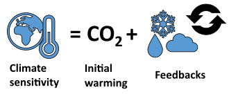
Diagram of factors that determine climate sensitivity. After increasing CO
2 levels, there is an initial warming. This warming gets amplified by the net effect of feedbacks. Self-reinforcing feedbacks include the melting of sunlight-reflecting ice, and higher evaporation increasing average atmospheric water vapour (a greenhouse gas).

Climate sensitivity is a measure of how much the Earth's climate will cool or warm after a change in the climate system, for instance, how much it will warm for doubling in carbon dioxide (CO
2) concentrations. In technical terms, climate sensitivity is the average change in the Earth's surface temperature in response to changes in radiative forcing, the difference between incoming and outgoing energy on Earth. Climate sensitivity is a key measure in climate science, and a focus area for climate scientists, who want to understand the ultimate consequences of anthroprogenic climate change.

The Earth's surface warms as a direct consequence of increased atmospheric CO
2, as well as increased concentrations of other greenhouse gases such as nitrous oxide and methane. Increasing temperatures have secondary effects on the climate system, such as an increase in atmospheric water vapour, which is itself also a greenhouse gas. Because scientists do not know exactly how strong these climate feedbacks are, it is difficult to precisely predict the amount of warming that will result from a given increase in greenhouse gas concentrations. If climate sensitivity turns out to be on the high side of scientific estimates, the Paris Agreement goal of limiting global warming to below 2 °C (3.6 °F) will be difficult to achieve.

The two primary types of climate sensitivity are the shorter-term "transient climate response", the increase in global average temperature that is expected to have occurred at a time when the atmospheric CO
2 concentration has doubled; and "equilibrium climate sensitivity", the higher long-term increase in global average temperature expected to occur after the effects of a doubled CO
2 concentration have had time to reach a steady state. Climate sensitivity is typically estimated in three ways; using direct observations of temperature and levels of greenhouse gases taken during the industrial age; using indirectly estimated temperature and other measurements from the Earth's more distant past; and modelling the various aspects of the climate system with computers.

Background

The rate at which energy reaches Earth as sunlight, and leaves Earth as heat radiation to space, must balance, or the total amount of heat energy on the planet at any one time will rise or fall, resulting in a planet that is warmer or cooler overall. An imbalance between the rates of incoming and outgoing radiation energy is called radiative forcing. A warmer planet radiates heat to space faster, so eventually a new balance is reached, with a higher planetary temperature. However, the warming of the planet also has knock-on effects. These knock-on effects create further warming, in an exacerbating feedback loop. Climate sensitivity is a measure of how much temperature change a given amount of radiative forcing will cause.

Radiative forcing

Radiative forcing is generally defined as the imbalance between incoming and outgoing radiation at the top of the atmosphere. Radiative forcing is measured in Watts per square meter (W/m²), the average imbalance in energy per second for each square meter of the Earth's surface.

Changes to radiative forcing lead to long-term changes in global temperature. A number of factors can affect radiative forcing: increased downwelling radiation due to the greenhouse effect, variability in solar radiation due to changes in planetary orbit, changes in solar irradiance, direct and indirect effects caused by aerosols (for example changes in albedo due to cloud cover), and changes in land use (i.e. deforestation or loss of reflective ice cover). In contemporary research, radiative forcing by greenhouse gases is well understood. As of 2019, large uncertainties remain for aerosols.

Key numbers

Carbon dioxide (CO
2) levels rose from 280 parts per million (ppm) in the eighteenth century, when humans in the Industrial Revolution started burning significant amounts of fossil fuel such as coal, to over 415 ppm by 2020. As CO
2 is a greenhouse gas, it hinders heat energy from leaving the Earth's atmosphere. In 2016, atmospheric CO
2 levels had increased by 45% over preindustrial levels, and radiative forcing caused by increased CO
2 was already more than 50% higher than in preindustrial times (due to non-linear effects). Between the start of the Industrial Revolution in the eighteenth century and 2020, the Earth's temperature rose by a little over one degree Celsius (about two degrees Fahrenheit).

Societal importance

Because the economics of climate change mitigation depend a lot on how quickly carbon neutrality needs to be achieved, climate sensitivity estimates can have important economic and policy-making implications. One study suggests that halving the uncertainty of the value for transient climate response (TCR) could save trillions of dollars. Scientists are uncertain about the precision of estimates of greenhouse gas increases on future temperature – a higher climate sensitivity would mean more dramatic increases in temperature – which makes it more prudent to take significant climate action. If climate sensitivity turns out to be on the high end of what scientists estimate, it will be impossible to achieve the Paris Agreement goal of limiting global warming to well below 2 °C; temperature increases will exceed that limit, at least temporarily. One study estimated that emissions cannot be reduced fast enough to meet the 2 °C goal if equilibrium climate sensitivity (the long-term measure) is higher than 3.4 °C (6.1 °F). The more sensitive the climate system is to changes in greenhouse gas concentrations, the more likely it is to have decades when temperatures are much higher or much lower than the longer-term average.

Contributors to climate sensitivity

Radiative forcing is one component of climate sensitivity. The radiative forcing caused by a doubling of atmospheric CO
2 levels (from the preindustrial 280 ppm) is approximately 3.7 watts per square meter (W/m²). In the absence of feedbacks, this energy imbalance would eventually result in roughly 1 °C (1.8 °F) of global warming. This figure is straightforward to calculate using the Stefan-Boltzmann law and is undisputed.

A further contribution arises from climate feedbacks, both exacerbating and suppressing. The uncertainty in climate sensitivity estimates is due entirely to modeling of feedbacks in the climate system, including water vapour feedback, ice-albedo feedback, cloud feedback, and lapse rate feedback. Suppressing feedbacks tend to counteract warming, increasing the rate at which energy is radiated to space from a warmer planet. Exacerbating feedbacks increase warming; for example, higher temperatures can cause ice to melt, reducing the ice area and the amount of sunlight the ice reflects, resulting in less heat energy being radiated back into space. Climate sensitivity depends on the balance between these feedbacks.

Measures of climate sensitivity

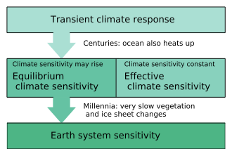
Schematic of how different measures of climate sensitivity relate to one another

Depending on the time scale, there are two main ways to define climate sensitivity: the short-term transient climate response (TCR) and the long-term equilibrium climate sensitivity (ECS), which both incorporate the warming from exacerbating feedback loops. These are not discrete categories; they overlap. Sensitivity to atmospheric CO
2 increases is measured in the amount of temperature change for doubling in the atmospheric CO
2 concentration.

Although "climate sensitivity" is usually used for the sensitivity to radiative forcing caused by rising atmospheric CO
2, it is a general property of the climate system. Other agents can also cause a radiative imbalance. Climate sensitivity is the change in surface air temperature per unit change in radiative forcing, and the climate sensitivity parameter is therefore expressed in units of °C/(W/m²). Climate sensitivity is approximately the same, whatever the reason for the radiative forcing (e.g. from greenhouse gases or solar variation). When climate sensitivity is expressed as the temperature change for a level of atmospheric CO
2 double the pre-industrial level, its units are degrees Celsius (°C).

Transient climate response

The transient climate response (TCR) is defined as "is the change in the global mean surface temperature, averaged over a 20-year period, centered at the time of atmospheric carbon dioxide doubling, in a climate model simulation" in which the atmospheric CO
2 concentration is increasing at 1% per year. This estimate is generated using shorter-term simulations. The transient response is lower than the equilibrium climate sensitivity, because slower feedbacks, which exacerbate the temperature increase, take more time to respond in full to an increase in the atmospheric CO
2 concentration. For instance, the deep ocean takes many centuries to reach a new steady state after a perturbation; during this time, it continues to serve as heatsink, cooling the upper ocean. The IPCC literature assessment estimates that TCR likely lies between 1 °C (1.8 °F) and 2.5 °C (4.5 °F).

A related measure is the transient climate response to cumulative carbon emissions (TCRE), which is the globally averaged surface temperature change after 1000 GtC of CO
2 has been emitted. As such, it includes not only temperature feedbacks to forcing, but also the carbon cycle and carbon cycle feedbacks.

Equilibrium climate sensitivity

The equilibrium climate sensitivity (ECS) is the long-term temperature rise (equilibrium global mean near-surface air temperature) that is expected to result from a doubling of the atmospheric CO
2 concentration (ΔT_2×). It is a prediction of the new global mean near-surface air temperature once the CO
2 concentration has stopped increasing and most of the feedbacks have had time to have their full effect. Reaching an equilibrium temperature can take centuries, or even millennia, after CO
2 has doubled. ECS is higher than TCR due to the oceans' short-term buffering effects. Computer models are used to estimate ECS. A comprehensive estimate means modelling the whole time span during which significant feedbacks continue to change global temperatures in the model; for instance, fully equilibrating ocean temperatures requires running a computer model that covers thousands of years. There are, however, less computing-intensive methods.

The IPCC Fifth Assessment Report (AR5) stated that "there is high confidence that ECS is extremely unlikely to be less than 1 °C and medium confidence that the ECS is likely between 1.5 °C and 4.5 °C and very unlikely greater than 6 °C". The long time scales involved with ECS make it arguably a less relevant measure for policy decisions around climate change.

Effective climate sensitivity

A common approximation to ECS is the effective equilibrium climate sensitivity. The effective climate sensitivity is an estimate of equilibrium climate sensitivity using data from a climate system, either in a model or real-world observations, that is not yet in equilibrium. Estimates assume that the net amplification effect of feedbacks (as measured after some period of warming) will remain constant afterwards. This is not necessarily true, as feedbacks can change with time. In many climate models, feedbacks become stronger over time, so that the effective climate sensitivity is lower than the real ECS.

Earth system sensitivity

By definition, equilibrium climate sensitivity does not includes feedbacks that take millennia to emerge, such as long-term changes in Earth's albedo due to changes in ice sheets and vegetation. It does include the slow response of the deep ocean warming up, which also takes millennia, and as such ECS doesn't reflect the actual future warming that would occur if CO
2 is stabilized at double pre-industrial values. Earth system sensitivity (ESS) incorporates the effects of these slower feedback loops, such as the change in Earth's albedo from the melting of large continental ice sheets (which covered much of the northern hemisphere during the Last Glacial Maximum, and currently cover Greenland and Antarctica). Changes in albedo as a result of vegetation changes, and changes in ocean circulations are also included. These longer-term feedback loops make the ESS larger than the ECS – possibly twice as large. Data from Earth's geological history is used to estimate ESS. Differences between modern and long-past climatic conditions mean that estimates of future ESS are highly uncertain. Like for ECS and TCR, the carbon cycle is not included in the definition of ESS, but all other elements of the climate system are.

Sensitivity to nature of the forcing

Different forcing agents, such as greenhouse gases and aerosols, can be compared using their radiative forcing (which is the initial radiative imbalance averaged over the entire globe). Climate sensitivity is the amount of warming per radiative forcing. To a first approximation, it does not matter the cause of the radiative imbalance is, whether it is greenhouse gases or something else. However, radiative forcing from sources other than CO
2 can cause a somewhat larger or smaller surface warming than a similar radiative forcing due to CO
2; the amount of feedback varies, mainly because these forcings are not uniformly distributed over the globe. Forcings that initially warm the northern hemisphere, land, or polar regions more strongly are systematically more effective at changing temperatures than an equivalent forcing due to CO
2, whose forcing is more uniformly distributed over the globe. This is because these regions have more self-reinforcing feedbacks, such as the ice-albedo feedback. Several studies indicate that human-emitted aerosols are more effective than CO
2 at changing global temperatures, while volcanic forcing is less effective. When climate sensitivity to CO
2 forcing is estimated using historical temperature and forcing (caused by a mix of aerosols and greenhouse gases), and this effect is not taken into account, climate sensitivity will be underestimated.

State dependence

Artist impression of a snowball Earth state.

While climate sensitivity has been defined as the short- or long-term temperature change resulting from any doubling of CO
2, there is evidence that the sensitivity of Earth's climate system is not constant. For instance, the planet has polar ice and high-altitude glaciers. Until the world's ice has completely melted, an exacerbating ice-albedo feedback loop makes the system more sensitive overall. Throughout Earth's history, there are thought to have been multiple periods where snow and ice covered almost the entire globe. In most models of this "snowball Earth" state, parts of the tropics were at least intermittently free of ice cover. As the ice was advancing or retreating, climate sensitivity would have been very high, as the large changes in area of ice cover would have made for a very strong ice-albedo feedback. Volcanic atmospheric composition changes are thought to have provided the radiative forcing needed to escape the snowball state.

Equilibrium climate sensitivity can change with climate.

Throughout the Quaternary period (the most recent 2.58 million years), climate has oscillated between glacial periods, of which the most recent was the Last Glacial Maximum, and interglacial periods, of which the most recent is the current Holocene, but climate sensitivity is difficult to determine in this period. The Paleocene–Eocene Thermal Maximum, circa 55.5 million years ago, was unusually warm, and may have been characterized by above-average climate sensitivity.

Climate sensitivity may further change if tipping points are crossed. It is unlikely that tipping points will cause short-term changes in climate sensitivity. If a tipping point is crossed, climate sensitivity is expected to change at the time scale of the subsystem that is hitting its tipping point. Especially if there are multiple interacting tipping points, the transition of climate to a new state may be difficult to reverse.

The two most used definitions of climate sensitivity specify the climate state: ECS and TCR are defined for a doubling with respect to the CO
2 levels in the pre-industrial era. Because of potential changes in climate sensitivity, the climate system may warm by a different amount after a second doubling of CO
2 than after a first doubling. The effect of any change in climate sensitivity is expected to be small or negligible in the first century after additional CO
2 is released into the atmosphere.

Estimating climate sensitivity

Historical estimates

Svante Arrhenius, in the 19th century, was the first person to quantify global warming as a consequence of a doubling of CO
2 concentration. In his first paper on the matter, he estimated that global temperature would rise by around 5 to 6 °C (9.0 to 10.8 °F) if the quantity of CO
2 was doubled. In later work, he revised this estimate to 4 °C (7.2 °F). Arrhenius used Samuel Pierpont Langley's observations of radiation emitted by the full moon to estimate the amount of radiation that was absorbed by water vapour and CO
2. To account for water vapour feedback, he assumed that relative humidity would stay the same under global warming.

The first calculation of climate sensitivity using detailed measurements of absorption spectra, and the first to use a computer to numerically integrate the radiative transfer through the atmosphere, was performed by Syukuro Manabe and Richard Wetherald in 1967. Assuming constant humidity, they computed an equilibrium climate sensitivity of 2.3 °C per doubling of CO
2 (which they rounded to 2 °C, the value most often quoted from their work, in the abstract of the paper). This work has been called "arguably the greatest climate-science paper of all time" and "the most influential study of climate of all time."

A committee on anthropogenic global warming, convened in 1979 by the United States National Academy of Sciences and chaired by Jule Charney, estimated equilibrium climate sensitivity to be 3 °C (5.4 °F), plus or minus 1.5 °C (2.7 °F). The Manabe and Wetherald estimate (2 °C (3.6 °F)), James E. Hansen's estimate of 4 °C (7.2 °F), and Charney's model were the only models available in 1979. According to Manabe, speaking in 2004, "Charney chose 0.5 °C as a reasonable margin of error, subtracted it from Manabe's number, and added it to Hansen's, giving rise to the 1.5 to 4.5 °C (2.7 to 8.1 °F) range of likely climate sensitivity that has appeared in every greenhouse assessment since ...." In 2008, climatologist Stefan Rahmstorf said: "At that time [it was published], the [Charney report estimate's] range [of uncertainty] was on very shaky ground. Since then, many vastly improved models have been developed by a number of climate research centers around the world."

Intergovernmental Panel on Climate Change

Historical estimates of climate sensitivity from the IPCC assessments. The first three reports gave a qualitative likely range, while the fourth and fifth assessment report formally quantified the uncertainty. The dark blue range is judged as being more than 66% likely.

Despite considerable progress in the understanding of Earth's climate system, assessments continued to report similar uncertainty ranges for climate sensitivity for some time after the 1979 Charney report. The 1990 IPCC First Assessment Report estimated that equilibrium climate sensitivity to a doubling of CO
2 lay between 1.5 and 4.5 °C (2.7 and 8.1 °F), with a "best guess in the light of current knowledge" of 2.5 °C (4.5 °F). This report used models with simplified representations of ocean dynamics. The IPCC supplementary report, 1992, which used full-ocean circulation models, saw "no compelling reason to warrant changing" the 1990 estimate; and the IPCC Second Assessment Report said that "No strong reasons have emerged to change [these estimates]". In these reports, much of the uncertainty around climate sensitivity was attributed to insufficient knowledge of cloud processes. The 2001 IPCC Third Assessment Report also retained this likely range.

Authors of the 2007 IPCC Fourth Assessment Report stated that confidence in estimates of equilibrium climate sensitivity had increased substantially since the Third Annual Report. The IPCC authors concluded that ECS is very likely to be greater than 1.5 °C (2.7 °F) and likely to lie in the range 2 to 4.5 °C (3.6 to 8.1 °F), with a most likely value of about 3 °C (5.4 °F). The IPCC stated that, due to fundamental physical reasons and data limitations, a climate sensitivity higher than 4.5 °C (8.1 °F) could not be ruled out, but that the climate sensitivity estimates in the likely range agreed better with observations and proxy climate data.

The 2013 IPCC Fifth Assessment Report reverted to the earlier range of 1.5 to 4.5 °C (2.7 to 8.1 °F) (with high confidence), because some estimates using industrial-age data came out low. (See the next section for details.) The report also stated that ECS is extremely unlikely to be less than 1 °C (1.8 °F) (high confidence), and is very unlikely to be greater than 6 °C (11 °F) (medium confidence). These values were estimated by combining the available data with expert judgement.

When the Ipcc begun to produce its IPCC Sixth Assessment Report many climate models begun to show higher climate sensitivity. The estimates for Equilibrium Climate Sensitivity changed from 3.2 °C to 3.7 °C and the estimates for the Transient climate response from 1.8 °C, to 2.0 °C. This is probably due to better understanding of the role of clouds and aerosols.

Methods of estimation

Using industrial-age (1750–present) data

Climate sensitivity can be estimated using observed temperature rise, observed ocean heat uptake, and modelled or observed radiative forcing. These data are linked though a simple energy-balance model to calculate climate sensitivity. Radiative forcing is often modelled, because Earth observation satellites that measure it existed during only part of the industrial age (only since the mid-20th century). Estimates of climate sensitivity calculated using these global energy constraints have consistently been lower than those calculated using other methods, around 2 °C (3.6 °F) or lower.

Estimates of transient climate response (TCR) calculated from models and observational data can be reconciled if it is taken into account that fewer temperature measurements are taken in the polar regions, which warm more quickly than the Earth as a whole. If only regions for which measurements are available are used in evaluating the model, differences in TCR estimates are negligible.

A very simple climate model could estimate climate sensitivity from industrial-age data by waiting for the climate system to reach equilibrium and then measuring the resulting warming, ΔT_eq (°C). Computation of the equilibrium climate sensitivity, S (°C), using the radiative forcing ΔF (W/m²) and the measured temperature rise, would then be possible. The radiative forcing resulting from a doubling of CO
2, F_{2${\displaystyle \times }$CO2}, is relatively well known, at about 3.7 W/m². Combining this information results in the following equation:

${\displaystyle S=\Delta T_{eq}\times F_{2\times CO_{2}}/\Delta F}$.

However, the climate system is not in equilibrium. Actual warming lags the equilibrium warming, largely because the oceans take up heat and will take centuries or millennia to reach equilibrium. Estimating climate sensitivity from industrial-age data requires an adjustment to the equation above. The actual forcing felt by the atmosphere is the radiative forcing minus the ocean's heat uptake, H (W/m²), so that climate sensitivity can be estimated by:

${\displaystyle S=\Delta T\times F_{2\times CO_{2}}/(\Delta F-H).}$

The global temperature increase between the beginning of the industrial period (taken as 1750) and 2011 was about 0.85 °C (1.53 °F). In 2011, the radiative forcing due to CO
2 and other long-lived greenhouse gases – mainly methane, nitrous oxide, and chlorofluorocarbons – emitted since the eighteenth century was roughly 2.8 W/m². The climate forcing, ΔF, also contains contributions from solar activity (+0.05 W/m²), aerosols (−0.9 W/m²), ozone (+0.35 W/m²), and other smaller influences, bringing the total forcing over the industrial period to 2.2 W/m², according to the best estimate of the IPCC AR5, with substantial uncertainty. The ocean heat uptake estimated by the IPCC AR5 as 0.42 W/m², yields a value for S of 1.8 °C (3.2 °F).

Other strategies

In theory, industrial-age temperatures could also be used to determine a timescale for the temperature response of the climate system, and thus climate sensitivity: if the effective heat capacity of the climate system is known, and the timescale is estimated using autocorrelation of the measured temperature, an estimate of climate sensitivity can be derived. In practice, however, simultaneous determination of the timescale and heat capacity is difficult.

Attempts have been made to use the 11-year solar cycle to constrain the transient climate response. Solar irradiance is about 0.9 W/m² higher during a solar maximum than during a solar minimum, and the effects of this can be observed in measured average global temperatures over the period 1959–2004. Unfortunately, the solar minima in this period coincided with volcanic eruptions, which have a cooling effect on the global temperature. Because the eruptions caused a larger and less well quantified decrease in radiative forcing than the reduced solar irradiance, it is questionable whether useful quantitative conclusions can be derived from the observed temperature variations.

Observations of volcanic eruptions have also been used to try to estimate climate sensitivity, but as the aerosols from a single eruption last at most a couple of years in the atmosphere, the climate system can never come close to equilibrium, and there is less cooling than there would be if the aerosols stayed in the atmosphere for longer. Therefore, volcanic eruptions give information only about a lower bound on transient climate sensitivity.

Using data from Earth's past

Historical climate sensitivity can be estimated by using reconstructions of Earth's past temperatures and CO
2 levels. Paleoclimatologists have studied different geological periods, such as the warm Pliocene (5.3 to 2.6 million years ago) and the colder Pleistocene (2.6 million to 11,700 years ago), seeking periods that are in some way analogous to or informative about current climate change. Climates further back in Earth's history are more difficult to study, because less data is available about them. For instance, past CO
2 concentrations can be derived from air trapped in ice cores, but as of 2020, the oldest continuous ice core is less than one million years old. Recent periods, such as the Last Glacial Maximum (LGM) (about 21,000 years ago) and the Mid-holocene (about 6,000 years ago), are often studied, especially when more information about them becomes available.

A 2007 estimate of sensitivity made using data from the most recent 420 million years is consistent with sensitivities of current climate models and with other determinations. The Paleocene–Eocene Thermal Maximum (about 55.5 million years ago), a 20,000-year period during which massive amount of carbon entered the atmosphere and average global temperatures increased by approximately 6 °C (11 °F), also provides a good opportunity to study the climate system when it was in a warm state. Studies of the last 800,000 years have concluded that climate sensitivity was greater in glacial periods than in interglacial periods.

As the name suggests, the LGM was a lot colder than today; there is good data on atmospheric CO
2 concentrations and radiative forcing during that period. While orbital forcing was different from that of the present, it had little effect on mean annual temperatures. Estimating climate sensitivity from the LGM can be done in several different ways. One way is to use estimates of global radiative forcing and temperature directly. The set of feedback mechanisms active during the LGM, however, may be different from the feedbacks caused by a doubling of CO
2 in the present, introducing additional uncertainty. In a different approach, a model of intermediate complexity is used to simulate conditions during the LGM. Several versions of this single model are run, with different values chosen for uncertain parameters, such that each version has a different ECS. Outcomes that best simulate observed cooling during the LGM probably produce the most realistic ECS values.

Using climate models

Frequency distribution of equilibrium climate sensitivity, based on simulations of doubling CO
2. Each model simulation has different estimates for processes that scientists do not sufficiently understand. Few of the simulations result in less than 2 °C (3.6 °F) of warming or significantly more than 4 °C (7.2 °F). However, the positive skew, which is also found in other studies, suggests that if carbon dioxide concentrations double, the probability of large or very large increases in temperature is greater than the probability of small increases.

Climate models are used to simulate the CO
2-driven warming of the future as well as the past. They operate on principles similar to those underlying models that predict the weather, but they focus on longer-term processes. Climate models typically begin with a starting state, then apply physical laws and knowledge about biology to generate subsequent states. As with weather modeling, no computer has the power to model the full complexity of the entire planet, so simplifications are used to reduce this complexity to something manageable. An important simplification divides Earth's atmosphere into model cells. For instance, the atmosphere might be divided into cubes of air ten or one hundred kilometers on a side. Each model cell is treated as if it were homogeneous. Calculations for model cells are much faster than trying to simulate each molecule of air separately.

A lower model resolution (large model cells, long time steps) takes less computing power, but it cannot simulate the atmosphere in as much detail. A model is unable able to simulate processes smaller than the model cells or shorter-term than a single time step. The effects of these smaller-scale (and shorter-term) processes must therefore be estimated using other methods. Physical laws contained in the models may also be simplified to speed up calculations. The biosphere must be included in climate models. The effects of the biosphere are estimated using data on the average behaviour of the average plant assemblage of an area under the modelled conditions. Climate sensitivity is therefore an emergent property of these models; it is not prescribed, but follows from the interaction of all the modelled processes.

To estimate climate sensitivity, a model is run using a variety of radiative forcings (doubling quickly, doubling gradually, or following historical emissions) and the temperature results are compared to the forcing applied. Different models give different estimates of climate sensitivity, but they tend to fall within a similar range, as described above.

Testing, comparisons, and estimates

Modelling of the climate system can lead to a wide range of outcomes. Models are often run using different plausible parameters in their approximation of physical laws and the behaviour of the biosphere, forming a perturbed physics ensemble that attempts to model the sensitivity of the climate to different types and amounts of change in each parameter. Alternatively, structurally different models developed at different institutions are put together, creating an ensemble. By selecting only those simulations that can simulate some part of the historical climate well, a constrained estimate of climate sensitivity can be made. One strategy for obtaining more accurate results is placing more emphasis on climate models that perform well in general.

A model is tested using observations, paleoclimate data, or both to see if it replicates them accurately. If it does not, inaccuracies in the physical model and parametrizations are sought and the model is modified. For models used to estimate climate sensitivity, specific test metrics that are directly and physically linked to climate sensitivity are sought; examples of such metrics are the global patterns of warming, the ability of a model to reproduce observed relative humidity in the tropics and subtropics, patterns of heat radiation, and the variability of temperature around long-term historical warming. Ensemble climate models developed at different institutions tend to produce constrained estimates of ECS that are slightly higher than 3 °C (5.4 °F); the models with ECS slightly above 3 °C (5.4 °F) simulate the above situations better than models with a lower climate sensitivity.

Many projects and groups exist which compare and analyse the results of multiple models. For instance, the Coupled Model Intercomparison Project (CMIP) has been running since the 1990s.

In preparation for the 2021 6th IPCC report, a new generation of climate models have been developed by scientific groups around the world. The average estimated climate sensitivity has increased in Coupled Model Intercomparison Project phase 6 (CMIP6) compared to the previous generation, with values spanning 1.8 to 5.6 °C (3.2 to 10.1 °F) across 27 global climate models and exceeding 4.5 °C (8.1 °F) in 10 of them. The cause of the increased ECS lies mainly in improved modelling of clouds; temperature rises are now believed to cause sharper decreases in the number of low clouds, and fewer low clouds means more sunlight is absorbed by the planet rather than reflected back into space. Models with the highest ECS values, however, are not consistent with observed warming.

Subsidy

From Wikipedia, the free encyclopedia

A subsidy or government incentive is a form of financial aid or support extended to an economic sector (business, or individual) generally with the aim of promoting economic and social policy.

Although commonly extended from the government, the term subsidy can relate to any type of support – for example from NGOs or as implicit subsidies. Subsidies come in various forms including: direct (cash grants, interest-free loans) and indirect (tax breaks, insurance, low-interest loans, accelerated depreciation, rent rebates).

Furthermore, they can be broad or narrow, legal or illegal, ethical or unethical. The most common forms of subsidies are those to the producer or the consumer. Producer/production subsidies ensure producers are better off by either supplying market price support, direct support, or payments to factors of production. Consumer/consumption subsidies commonly reduce the price of goods and services to the consumer. For example, in the US at one time it was cheaper to buy gasoline than bottled water.

Types

Production subsidy

A production subsidy encourages suppliers to increase the output of a particular product by partially offsetting the production costs or losses. The objective of production subsidies is to expand production of a particular product more so that the market would promote but without raising the final price to consumers. This type of subsidy is predominantly found in developed markets. Other examples of production subsidies include the assistance in the creation of a new firm (Enterprise Investment Scheme), industry (industrial policy) and even the development of certain areas (regional policy). Production subsidies are critically discussed in the literature as they can cause many problems including the additional cost of storing the extra produced products, depressing world market prices, and incentivizing producers to over-produce, for example, a farmer overproducing in terms of his land's carrying capacity.

Consumer/consumption subsidy

A consumption subsidy is one that subsidizes the behavior of consumers. This type of subsidies are most common in developing countries where governments subsidise such things as food, water, electricity and education on the basis that no matter how impoverished, all should be allowed those most basic requirements. For example, some governments offer 'lifeline' rates for electricity, that is, the first increment of electricity each month is subsidized. Evidence from recent studies suggests that government expenditures on subsidies remain high in many countries, often amounting to several percentage points of GDP. Subsidization on such a scale implies substantial opportunity costs. There are at least three compelling reasons for studying government subsidy behavior. First, subsidies are a major instrument of government expenditure policy. Second, on a domestic level, subsidies affect domestic resource allocation decisions, income distribution, and expenditure productivity. A consumer subsidy is a shift in demand as the subsidy is given directly to consumers.

Export subsidy

An export subsidy is a support from the government for products that are exported, as a means of assisting the country's balance of payments. Usha Haley and George Haley identified the subsidies to manufacturing industry provided by the Chinese government and how they have altered trade patterns. Traditionally, economists have argued that subsidies benefit consumers but hurt the subsidizing countries. Haley and Haley provided data to show that over the decade after China joined the World Trade Organization industrial subsidies have helped give China an advantage in industries in which they previously enjoyed no comparative advantage such as the steel, glass, paper, auto parts, and solar industries. China’s shores have also collapsed from overfishing and industrialization, which is why the Chinese government heavily subsidizes its fishermen, who sail the world in search of new grounds.

Export subsidy is known for being abused. For example, some exporters substantially over declare the value of their goods so as to benefit more from the export subsidy. Another method is to export a batch of goods to a foreign country but the same goods will be re-imported by the same trader via a circuitous route and changing the product description so as to obscure their origin. Thus the trader benefits from the export subsidy without creating real trade value to the economy. Export subsidy as such can become a self-defeating and disruptive policy.

Import subsidy

An import subsidy is support from the government for products that are imported. Rarer than an export subsidy, an import subsidy further reduces the price to consumers for imported goods. Import subsidies have various effects depending on the subject. For example, consumers in the importing country are better off and experience an increase in consumer welfare due to the decrease in price of the imported goods, as well as the decrease in price of the domestic substitute goods. Conversely, the consumers in the exporting country experience a decrease in consumer welfare due to an increase in the price of their domestic goods. Furthermore, producers of the importing country experience a loss of welfare due to a decrease of the price for the good in their market, while on the other side, the exporters of the producing country experience an increase in well being due to the increase in demand. Ultimately, the import subsidy is rarely used due to an overall loss of welfare for the country due to a decrease in domestic production and a reduction in production throughout the world. However, that can result in a redistribution of income.

Employment subsidy

An employment subsidy serves as an incentive to businesses to provide more job opportunities to reduce the level of unemployment in the country (income subsidies) or to encourage research and development. With an employment subsidy, the government provides assistance with wages. Another form of employment subsidy is the social security benefits. Employment subsidies allow a person receiving the benefit to enjoy some minimum standard of living.

Tax subsidy

Governments can create the same outcome through selective tax breaks as through cash payments. For example, if a government sends monetary assistance that reimburses 15% of all health expenditures to a group that is paying 15% income tax. Exactly the same subsidy is achieved by giving a health tax deduction. Tax subsidies are also known as tax expenditures.

Tax breaks are often considered to be a subsidy. Like other subsidies, they distort the economy; but tax breaks are also less transparent, and are difficult to undo.

The Multilateral Convention to Implement Tax Treaty Related Measures to Prevent Base Erosion and Profit Shifting is a treaty signed by half the nations of the world and it is aimed to prevent Base Erosion and Profit Shifting, a particular form of tax subsidy related to Intellectual Property.

Transport subsidies

Some governments subsidise transport, especially rail and bus transport, which decrease congestion and pollution compared to cars. In the EU, rail subsidies are around €73 billion, and Chinese subsidies reach $130 billion.

Publicly-owned airports can be an indirect subsidy if they lose money. The European Union, for instance, criticizes Germany for its high number of money-losing airports that are used primarily by low cost carriers, characterizing the arrangement as an illegal subsidy.

In many countries, roads and highways are paid for through general revenue, rather than tolls or other dedicated sources that are paid only by road users, creating an indirect subsidy for road transportation. The fact that long-distance buses in Germany do not pay tolls has been called an indirect subsidy by critics, who point to track access charges for railways.

Oil subsidies

An oil subsidy is one aimed at decreasing the overall price of oil. Oil subsidies have always played a major part in U.S. history. These began as early as World War I and have increased in the following decades. However, due to changes in the perceptions of the environment, in 2012 President Barack Obama ended the subsidies to the oil industry, which were, at the time, $4 billion. The Secretary-General of the United Nations António Guterres called for an end of subsidies for fossil fuels.

Housing subsidies

Housing subsidies are designed to promote the construction industry and homeownership. As of 2018, U.S housing subsidies total around $15 billion per year. Housing subsidies can come in two types; assistance with down payment and interest rate subsidies. The deduction of mortgage interest from the federal income tax accounts for the largest interest rate subsidy. Additionally, the federal government will help low-income families with the down payment, coming to $10.9 million in 2008.

Environmental externalities

As well as the conventional and formal subsidies as outlined above there are myriad implicit subsidies principally in the form of environmental externalities. These subsidies include anything that is omitted but not accounted for and thus is an externality. These include things such as car drivers who pollute everyone's atmosphere without compensating everyone, farmers who use pesticides which can pollute everyone's ecosystems, again without compensating everyone, or Britain's electricity production which results in additional acid rain in Scandinavia. In these examples the polluter is effectively gaining a net benefit but not compensating those affected. Although they are not subsidies in the form of direct economic support from a government, they are no less economically, socially and environmentally harmful.

A 2015 report studied the implicit subsidies accruing to 20 fossil fuel companies and found that, while highly profitable, the hidden economic cost to society was also large. The report spans the period 2008–2012 and notes that: "for all companies and all years, the economic cost to society of their CO
2 emissions was greater than their after‐tax profit, with the single exception of ExxonMobil in 2008." Pure coal companies fare even worse: "the economic cost to society exceeds total revenue (employment, taxes, supply purchases, and indirect employment) in all years, with this cost varying between nearly $2 and nearly $9 per $1 of revenue."

Categorising subsidies

Broad and narrow

These various subsidies can be divided into broad and narrow. Narrow subsidies are those monetary transfers that are easily identifiable and have a clear intent. They are commonly characterised by a monetary transfer between governments and institutions or businesses and individuals. A classic example is a government payment to a farmer.

Conversely broad subsidies include both monetary and non-monetary subsidies and is often difficult to identify. A broad subsidy is less attributable and less transparent. Environmental externalities are the most common type of broad subsidy.

Economic effects

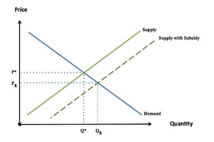
Competitive equilibrium is a state of balance between buyers and suppliers, in which the quantity demanded of a good is the quantity supplied at a specified price. When the quantity demand exceeds the equilibrium quantity, price falls; conversely, a reduction in the supply of a good beyond equilibrium quantity implies an increase in the price. The effect of a subsidy is to shift the supply or demand curve to the right (i.e. increases the supply or demand) by the amount of the subsidy. If a consumer is receiving the subsidy, a lower price of a good resulting from the marginal subsidy on consumption increases demand, shifting the demand curve to the right. If a supplier is receiving the subsidy, an increase in the price (revenue) resulting from the marginal subsidy on production results increases supply, shifting the supply curve to the right.

Assuming the market is in a perfectly competitive equilibrium, a subsidy increases the supply of the good beyond the equilibrium competitive quantity. The imbalance creates deadweight loss. Deadweight loss from a subsidy is the amount by which the cost of the subsidy exceeds the gains of the subsidy. The magnitude of the deadweight loss is dependent on the size of the subsidy. This is considered a market failure, or inefficiency.

Subsidies targeted at goods in one country, by lowering the price of those goods, make them more competitive against foreign goods, thereby reducing foreign competition. As a result, many developing countries cannot engage in foreign trade, and receive lower prices for their products in the global market. This is considered protectionism: a government policy to erect trade barriers in order to protect domestic industries. The problem with protectionism arises when industries are selected for nationalistic reasons (infant-industry), rather than to gain a comparative advantage. The market distortion, and reduction in social welfare, is the logic behind the World Bank policy for the removal of subsidies in developing countries.

Subsidies create spillover effects in other economic sectors and industries. A subsidized product sold in the world market lowers the price of the good in other countries. Since subsidies result in lower revenues for producers of foreign countries, they are a source of tension between the United States, Europe and poorer developing countries. While subsidies may provide immediate benefits to an industry, in the long-run they may prove to have unethical, negative effects. Subsidies are intended to support public interest, however, they can violate ethical or legal principles if they lead to higher consumer prices or discriminate against some producers to benefit others. For example, domestic subsidies granted by individual US states may be unconstitutional if they discriminate against out-of-state producers, violating the Privileges and Immunities Clause or the Dormant Commerce Clause of the United States Constitution. Depending on their nature, subsidies are discouraged by international trade agreements such as the World Trade Organization (WTO). This trend, however, may change in the future, as needs of sustainable development and environmental protection could suggest different interpretations regarding energy and renewable energy subsidies. In its July 2019 report, "Going for Growth 2019: The time for reform is now", the OECD suggests that countries make better use of environmental taxation, phase out agricultural subsidies and environmentally harmful tax breaks.

Perverse subsidies

Definitions

Although subsidies can be important, many are "perverse", in the sense of having adverse unintended consequences. To be "perverse", subsidies must exert effects that are demonstrably and significantly adverse both economically and environmentally. A subsidy rarely, if ever, starts perverse, but over time a legitimate efficacious subsidy can become perverse or illegitimate if it is not withdrawn after meeting its goal or as political goals change. Perverse subsidies are now so widespread that as of 2007 they amounted $2 trillion per year in the six most subsidised sectors alone (agriculture, fossil fuels, road transportation, water, fisheries and forestry).

Effects

The detrimental effects of perverse subsidies are diverse in nature and reach. Case-studies from differing sectors are highlighted below but can be summarised as follows.

Directly, they are expensive to governments by directing resources away from other legitimate should priorities (such as environmental conservation, education, health, or infrastructure), ultimately reducing the fiscal health of the government.

Indirectly, they cause environmental degradation (exploitation of resources, pollution, loss of landscape, misuse and overuse of supplies) which, as well as its fundamental damage, acts as a further brake on economies; tend to benefit the few at the expense of the many, and the rich at the expense of the poor; lead to further polarization of development between the Northern and Southern hemispheres; lower global market prices; and undermine investment decisions reducing the pressure on businesses to become more efficient. Over time the latter effect means support becomes enshrined in human behaviour and business decisions to the point where people become reliant on, even addicted to, subsidies, 'locking' them into society.

Consumer attitudes do not change and become out-of-date, off-target and inefficient; furthermore, over time people feel a sense of historical right to them.

Implementation

Perverse subsidies are not tackled as robustly as they should be. Principally, this is because they become 'locked' into society, causing bureaucratic roadblocks and institutional inertia. When cuts are suggested many argue (most fervently by those 'entitled', special interest groups and political lobbyists) that it will disrupt and harm the lives of people who receive them, distort domestic competitiveness curbing trade opportunities, and increase unemployment. Individual governments recognise this as a 'prisoner's dilemma' – insofar as that even if they wanted to adopt subsidy reform, by acting unilaterally they fear only negative effects will ensue if others do not follow. Furthermore, cutting subsidies, however perverse they may be, is considered a vote-losing policy.

Reform of perverse subsidies is at a propitious time. The current economic conditions mean governments are forced into fiscal constraints and are looking for ways to reduce activist roles in their economies. There are two main reform paths: unilateral and multilateral. Unilateral agreements (one country) are less likely to be undertaken for the reasons outlined above, although New Zealand, Russia, Bangladesh and others represent successful examples. Multilateral actions by several countries are more likely to succeed as this reduces competitiveness concerns, but are more complex to implement requiring greater international collaboration through a body such as the WTO. Irrespective of the path, the aim of policymakers should be to: create alternative policies that target the same issue as the original subsidies but better; develop subsidy removal strategies allowing market-discipline to return; introduce 'sunset' provisions that require remaining subsidies to be re-justified periodically; and make perverse subsidies more transparent to taxpayers to alleviate the 'vote-loser' concern.

Examples

Agricultural subsidies

Support for agriculture dates back to the 19th century. It was developed extensively in the EU and USA across the two World Wars and the Great Depression to protect domestic food production, but remains important across the world today. In 2005, US farmers received $14 billion and EU farmers $47 billion in agricultural subsidies. Today, agricultural subsidies are defended on the grounds of helping farmers to maintain their livelihoods. The majority of payments are based on outputs and inputs and thus favour the larger producing agribusinesses over the small-scale farmers. In the USA nearly 30% of payments go to the top 2% of farmers.

By subsidising inputs and outputs through such schemes as 'yield based subsidisation', farmers are encouraged to over-produce using intensive methods, including using more fertilizers and pesticides; grow high-yielding monocultures; reduce crop rotation; shorten fallow periods; and promote exploitative land use change from forests, rainforests and wetlands to agricultural land. These all lead to severe environmental degradation, including adverse effects on soil quality and productivity including erosion, nutrient supply and salinity which in turn affects carbon storage and cycling, water retention and drought resistance; water quality including pollution, nutrient deposition and eutrophication of waterways, and lowering of water tables; diversity of flora and fauna including indigenous species both directly and indirectly through the destruction of habitats, resulting in a genetic wipe-out.

Cotton growers in the US reportedly receive half their income from the government under the Farm Bill of 2002. The subsidy payments stimulated overproduction and resulted in a record cotton harvest in 2002, much of which had to be sold at very reduced prices in the global market. For foreign producers, the depressed cotton price lowered their prices far below the break-even price. In fact, African farmers received 35 to 40 cents per pound for cotton, while US cotton growers, backed by government agricultural payments, received 75 cents per pound. Developing countries and trade organizations argue that poorer countries should be able to export their principal commodities to survive, but protectionist laws and payments in the United States and Europe prevent these countries from engaging in international trade opportunities.

Fisheries

Today, much of the world's major fisheries are overexploited; in 2002, the WWF estimate this at approximately 75%. Fishing subsidies include "direct assistant to fishers; loan support programs; tax preferences and insurance support; capital and infrastructure programs; marketing and price support programs; and fisheries management, research, and conservation programs." They promote the expansion of fishing fleets, the supply of larger and longer nets, larger yields and indiscriminate catch, as well as mitigating risks which encourages further investment into large-scale operations to the disfavour of the already struggling small-scale industry. Collectively, these result in the continued overcapitalization and overfishing of marine fisheries.

There are four categories of fisheries subsidies. First are direct financial transfers, second are indirect financial transfers and services. Third, certain forms of intervention and fourth, not intervening. The first category regards direct payments from the government received by the fisheries industry. These typically affect profits of the industry in the short term and can be negative or positive. Category two pertains to government intervention, not involving those under the first category. These subsidies also affect the profits in the short term but typically are not negative. Category three includes intervention that results in a negative short-term economic impact, but economic benefits in the long term. These benefits are usually more general societal benefits such as the environment. The final category pertains to inaction by the government, allowing producers to impose certain production costs on others. These subsidies tend to lead to positive benefits in the short term but negative in the long term.

Others

The US National Football League's (NFL) profits have topped records at $11 billion, the highest of all sports. The NFL had tax-exempt status until voluntarily relinquishing it in 2015, and new stadiums have been built with public subsidies.

The Commitment to Development Index (CDI), published by the Center for Global Development, measures the effect that subsidies and trade barriers actually have on the undeveloped world. It uses trade, along with six other components such as aid or investment, to rank and evaluate developed countries on policies that affect the undeveloped world. It finds that the richest countries spend $106 billion per year subsidizing their own farmers – almost exactly as much as they spend on foreign aid.

Energy subsidy

From Wikipedia, the free encyclopedia

https://en.wikipedia.org/wiki/Energy_subsidy 

 

Fossil-fuel subsidies in 2015

 

Fossil-fuel subsidies per capita in 2015

Energy subsidies are measures that keep prices for customers below market levels, or for suppliers above market levels, or reduce costs for customers and suppliers. Energy subsidies may be direct cash transfers to suppliers, customers, or related bodies, as well as indirect support mechanisms, such as tax exemptions and rebates, price controls, trade restrictions, and limits on market access.

Eliminating fossil fuel subsidies would greatly reduce global carbon emissions and would reduce the health risks of air pollution.

Overview

Main arguments for energy subsidies are:

• Security of supply – subsidies are used to ensure adequate domestic supply by supporting indigenous fuel production in order to reduce import dependency, or supporting overseas activities of national energy companies.
• Environmental improvement – subsidies are used to reduce pollution, including different emissions, and to fulfill international obligations (e.g. Kyoto Protocol).
• Economic benefits – subsidies in the form of reduced prices are used to stimulate particular economic sectors or segments of the population, e.g. alleviating poverty and increasing access to energy in developing countries.
• Employment and social benefits – subsidies are used to maintain employment, especially in periods of economic transition.

Main arguments against energy subsidies are:

• Some energy subsidies counter the goal of sustainable development, as they may lead to higher consumption and waste, exacerbating the harmful effects of energy use on the environment, create a heavy burden on government finances and weaken the potential for economies to grow, undermine private and public investment in the energy sector. Also, most benefits from fossil fuel subsidies in developing countries go to the richest 20% of households.
• Impede the expansion of distribution networks and the development of more environmentally benign energy technologies, and do not always help the people that need them most.
• The study conducted by the World Bank finds that subsidies to the large commercial businesses that dominate the energy sector are not justified. However, under some circumstances it is reasonable to use subsidies to promote access to energy for the poorest households in developing countries. Energy subsidies should encourage access to the modern energy sources, not to cover operating costs of companies. The study conducted by the World Resources Institute finds that energy subsidies often go to capital intensive projects at the expense of smaller or distributed alternatives.

Types of energy subsidies are:

• Direct financial transfers – grants to suppliers; grants to customers; low-interest or preferential loans to suppliers.
• Preferential tax treatments – rebates or exemption on royalties, duties, supplier levies and tariffs; tax credit; accelerated depreciation allowances on energy supply equipment.
• Trade restrictions – quota, technical restrictions and trade embargoes.
• Energy-related services provided by government at less than full cost – direct investment in energy infrastructure; public research and development.
• Regulation of the energy sector – demand guarantees and mandated deployment rates; price controls; market-access restrictions; preferential planning consent and controls over access to resources.
• Failure to impose external costs – environmental externality costs; energy security risks and price volatility costs.
• Depletion Allowance – allows a deduction from gross income of up to ~27% for the depletion of exhaustible resources (oil, gas, minerals).

Overall, energy subsidies require coordination and integrated implementation, especially in light of globalization and increased interconnectedness of energy policies, thus their regulation at the World Trade Organization is often seen as necessary.

Impact of fossil fuel subsidies

The degree and impact of fossil fuel subsidies is extensively studied. Because fossil fuels are a leading contributor to climate change through greenhouse gases, fossil fuel subsidies increase emissions and exacerbate climate change. The OECD created an inventory in 2015 of subsidies for the extraction, refining, or combustion of fossil fuels among the OECD and large emerging economies. This inventory identified an overall value of $160 to $200 billion per year between 2010 and 2014. Meanwhile, the International Energy Agency has estimated global fossil fuel subsidies as ranging from $300 to $600 billion per year between 2008 and 2015.

According to the International Energy Agency, the elimination of fossil fuel subsidies worldwide would be one of the most effective ways of reducing greenhouse gases and battling global warming. Along with this, elimination of these subsidies was welcomed by the G20 nations as a way reduce expenditures during the recession during the 2009 Pittsburgh Summit. In May 2016, the G7 nations set for the first time a deadline for ending most fossil fuel subsidies; saying government support for coal, oil and gas should end by 2025. According to a 2019 report by the Overseas Development Institute, the G20 governments still provide billions of dollars of support for the production and consumption of fossil fuels, spending at least $63.9 billion per year on coal alone.

According to the OECD, subsidies supporting fossil fuels, particularly coal and oil, represent greater threats to the environment than subsidies to renewable energy. Subsidies to nuclear power contribute to unique environmental and safety issues, related mostly to the risk of high-level environmental damage, although nuclear power contributes positively to the environment in the areas of air pollution and climate change. According to Fatih Birol, Chief Economist at the International Energy Agency, without a phasing out of fossil fuel subsidies, countries will not reach their climate targets.

In 2011, IEA chief economist Fatih Birol said the current $409 billion equivalent of fossil fuel subsidies (in non-OECD countries) are encouraging a wasteful use of energy, and that the cuts in subsidies is the biggest policy item that would help renewable energies get more market share and reduce CO₂ emissions.

Environmental cost

Global fossil fuel subsidies reached $319 billion in 2017, although this number rises to $5.2 trillion (equivalent to 6.3% of world economy), when the economic value of environmental externalities such as air pollution are priced in. When measured this way, ending these subsidies can cause a 28% reduction in global carbon emissions and a 46% reduction in deaths due to fossil fuel air pollution. Total global air pollution deaths reach 7 million annually. Using this definition, "China was the biggest subsidizer in 2013 ($1.8 trillion), followed by the United States ($0.6 trillion), and Russia, the European Union, and India (each with about $0.3 trillion)."

IEA position on subsidies

According to International Energy Agency (IEA) (2011) energy subsidies artificially lower the price of energy paid by customers, raise the price received by suppliers or lower the cost of production. "Fossil fuels subsidies costs generally outweigh the benefits. Subsidies to renewables and low-carbon energy technologies can bring long-term economic and environmental benefits". In November 2011, an IEA report entitled Deploying Renewables 2011 said "subsidies in green energy technologies that were not yet competitive are justified in order to give an incentive to investing into technologies with clear environmental and energy security benefits". The IEA's report disagreed with claims that renewable energy technologies are only viable through costly subsidies and not able to produce energy reliably to meet demand. "A portfolio of renewable energy technologies is becoming cost-competitive in an increasingly broad range of circumstances, in some cases providing investment opportunities without the need for specific economic support," the IEA said, and added that "cost reductions in critical technologies, such as wind and solar, are set to continue."

Fossil-fuel consumption subsidies in non-OECD countries were $409 billion in 2010, oil products being half of it. In OECD countries, fossil fuel consumption subsidies have largely been phased out. Global fossil fuel taxes, mostly in OECD countries and on oil products, yield around $800 billion in revenues annually. Renewable energy is subsidized in order to compete in the market, increase their volume and develop the technology so that the subsidies become unnecessary with the development. Eliminating fossil-fuel subsidies could bring economic and environmental benefits. Phasing out fossil-fuel subsidies by 2020 would cut primary energy demand 5%. Since the start of 2010, at least 15 countries have taken steps to phase out fossil-fuel subsidies.

According to the IEA the phase-out of fossil fuel subsidies, over $500 billion annually, will reduce 10% greenhouse gas emissions by 2050.

Subsidies by country

The International Energy Agency estimates that governments subsidised fossil fuels by US $548 billion in 2013. Ten countries accounted for almost three-quarters of this figure. At their meeting in September 2009 the G-20 countries committed to "rationalize and phase out over the medium term inefficient fossil fuel subsidies that encourage wasteful consumption". The 2010s have seen many countries reducing energy subsidies, for instance in July 2014 Ghana abolished all diesel and gasoline subsidies, whilst in the same month Egypt raised diesel prices 63% as part of a raft of reforms intended to remove subsidies within 5 years.

The public energy subsidies for energy in Finland in 2013 were €700 million for fossil energy and €60 million for renewable energy (mainly wood and wind).

Canada

Fossil fuel subsidies

The Canadian federal government offers subsidies for fossil fuel exploration and production and Export Development Canada regularly provides financing to oil and gas companies. A 2018 report from the Overseas Development Institute, a UK-based think tank, found that Canada spent a greater proportion of its GDP on fiscal support to oil and gas production in 2015 and 2016 than any other G7 country.

In 2015 and 2016, the largest federal subsidies for fossil fuel exploration and production were the Canadian Exploration Expense (CEE), the Canadian Development Expense (CDE), and the Atlantic Investment Tax Credit (AITC). In these years Canada paid a yearly average of $1.018 billion CAD to oil and gas companies through the CDE, $148 million CAD through the CEE, and $127 million through the AITC. In 2017, subsidies to oil and gas through the AITC were phased out. Also in 2017, the federal government reformed the CEE so that exploration expenses may only be deducted through it if the exploration is unsuccessful. Otherwise, these expenses must be deducted through the CDE, which is deductible at 30% rather than 100%.

In December 2018, in response to low Canadian oil prices, the federal government announced $1.6 billion in financial support for the oil and gas sector: $1 billion in loans to oil and gas exporters from Export Development Canada, $500 million in financing for “higher risk” oil and gas companies from the Business Development Bank of Canada, $50 million through Natural Resources Canada’s Clean Growth Program, and $100 million through Innovation, Science and Economic Development Canada’s Strategic Innovation Fund. Minister of Natural Resources Amarjeet Sohi said that this financing is “not a subsidy for fossil fuels”, adding that “These are commercial loans, made available on commercial terms. We have committed to phasing out inefficient fossil fuel subsidies by 2025, and we stand by that commitment". In 2016, Canada committed to “phase out inefficient fossil fuel subsidies by 2025” in line with commitments made with G20 and G7 countries, although a 2017 report from the Office of the Auditor-General found that little work had been done to define this goal and establish a timeline for achieving it. Reducing subsidies to fossil fuels was an explicit part of the Liberal Party's platform in the 2015 federal election.

The largest provincial fossil fuel subsidies are paid by Alberta and British Columbia. Alberta spent a yearly average of $1.161 billion CAD on Crown Royalty Reductions for oil and gas from 2013 to 2015. And British Columbia paid a yearly average of $271 million CAD to gas companies through the Deep Drilling Credit.

Canadian provincial governments also offer subsidies for the consumption of fossil fuels. For example, Saskatchewan offers a fuel tax exemption for farmers and a sales tax exemption for natural gas used for heating.

A 2018 report from the Overseas Development Institute was critical of Canada's reporting and transparency practices around its fossil fuel subsidies. Canada does not publish specific reports on its fiscal support for fossil fuels, and when Canada’s Office of the Auditor-General attempted an audit of Canadian fossil fuel subsidies in 2017, they found much of the data they needed was not provided by Finance Canada. Export Development Canada reports on their transactions related to fossil fuel projects, but do not provide data on exact amounts or the stage of project development.

Iran

Contrary to the subsidy reform plan's objectives, under president Rouhani the volume of Iranian subsidies given to its citizens on fossil fuel increased 42.2% in 2019 and equals 15.3% of Iran’s GDP and 16% of total global energy subsidies. This has made Iran the world's largest subsidizer of energy prices. This situation is leading to highly wasteful consumption patterns, large budget deficits, price distortions in its entire economy, pollution and very lucrative (multi-billion dollars) contraband (because of price differentials) with neighbouring countries each year by rogue elements within the Iranian government supporting the status-quo.

Russia

Russia is one of the world’s energy powerhouses. It holds the world’s largest natural gas reserves (27% of total), the second-largest coal reserves, and the eighth-largest oil reserves. Russia is the world's third-largest energy subsidizer as of 2015. The country subsidizes electricity and natural gas as well as oil extraction. Approximately 60% of the subsidies go to natural gas, with the remainder spent on electricity (including under-pricing of gas delivered to power stations). For oil extraction the government gives tax exemptions and duty reductions amounting to about 22 billion dollars a year. Some of the tax exemptions and duty reductions also apply to natural gas extraction, though the majority is allocated for oil. In 2013 Russia offered the first subsidies to renewable power generators. The large subsidies of Russia are costly and it is recommended in order to help the economy that Russia lowers its domestic subsidies. However, the potential elimination of energy subsidies in Russia carries the risk of social unrest that makes Russian authorities reluctant to remove them.

Turkey

The energy policy of Turkey subsidizes fossil fuels US$1.6 billion annually including heavily subsidizing coal in Turkey.

United Kingdom

The government says that the 5% value added tax (VAT) rate on natural gas for home heating is not a subsidy, but some environmental groups disagree and say that it should be increased to the standard 20% with the extra revenue ringfenced for poor people.

United States

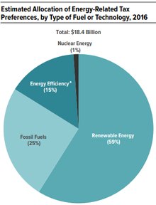
Congressional Budget Office estimated allocation of energy-related tax preferences, by type of fuel or technology, 2016

According to Congressional Budget Office testimony in 2016, an estimated $10.9 billion in tax preferences was directed toward renewable energy, $4.6 billion went to fossil fuels, and $2.7 billion went to energy efficiency or electricity transmission.

According to a 2015 estimate by the Obama administration, the US oil industry benefited from subsidies of about $4.6 billion per year. A 2017 study by researchers at Stockholm Environment Institute published in the journal Nature Energy estimated that nearly half of U.S. oil production would be unprofitable without subsidies.

Allocation of subsidies in the United States

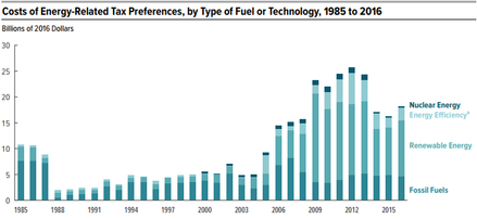
Congressional Budget Office testimony delivered March 29, 2017 showing the historic trend of energy related tax preferences

A 2017 study by the consulting firm Management Information Services, Inc. (MISI) estimated the total historical federal subsidies for various energy sources over the years 1950–2016. The study found that oil, natural gas, and coal received $414 billion, $140 billion, and $112 billion (2015 dollars), respectively, or 65% of total energy subsidies over that period. Oil, natural gas, and coal benefited most from percentage depletion allowances and other tax-based subsidies, but oil also benefited heavily from regulatory subsidies such as exemptions from price controls and higher-than-average rates of return allowed on oil pipelines. The MISI report found that non-hydro renewable energy (primarily wind and solar) benefited from $158 billion in federal subsidies, or 16% of the total, largely in the form of tax policy and direct federal expenditures on research and development (R&D). Nuclear power benefited from $73 billion in federal subsidies, 8% of the total and less than half of the total applied to renewables, while hydro power received $105 billion in federal subsidies, 10% of the total. Notable was MISI's finding that between 2011 through 2016, renewable energy received more than three times as much help in federal incentives as oil, natural gas, coal, and nuclear combined, and 27 times as much as nuclear energy.

In the United States, the federal government has paid US$145 billion for energy subsidies to support R&D for nuclear power ($85 billion) and fossil fuels ($60 billion) from 1950 to 2016. During this same timeframe, renewable energy technologies received a total of US $34 billion. Though in 2007 some suggested that a subsidy shift would help to level the playing field and support growing energy sectors, namely solar power, wind power, and bio-fuels., by 2017 those sources combined had yet to provide 10% of U.S. electricity, and intermittency forced utilities to remain reliant on oil, natural gas, and coal to meet baseload demand. Many of the "subsidies" available to the oil and gas industries are general business opportunity credits, available to all US businesses (particularly, the foreign tax credit mentioned above). The value of industry-specific (oil, gas, and coal) subsidies in 2006 was estimated by the Texas State Comptroller to be $6.25 billion - about 60% of the amount calculated by the Environmental Law Institute. The balance of federal subsidies, which the comptroller valued at $7.4 billion, came from shared credits and deductions, and oil defense (spending on the Strategic Petroleum Reserve, energy infrastructure security, etc.).

Critics allege that the most important subsidies to the nuclear industry have not involved cash payments, but rather the shifting of construction costs and operating risks from investors to taxpayers and ratepayers, burdening them with an array of risks including cost overruns, defaults to accidents, and nuclear waste management. Critics claim that this approach distorts market choices, which they believe would otherwise favor less risky energy investments.

Many energy analysts, such as Clint Wilder, Ron Pernick and Lester Brown, have suggested that energy subsidies need to be shifted away from mature and established industries and towards high growth clean energy (excluding nuclear). They also suggest that such subsidies need to be reliable, long-term and consistent, to avoid the periodic difficulties that the wind industry has had in the United States.

United States government role in the development of new energy industries

From civilian nuclear power to hydro, wind, solar, and shale gas, the United States federal government has played a central role in the development of new energy industries.

America's nuclear power industry, which currently supplies about 20% of the country's electricity, has its origins in the Manhattan Project to develop atomic weapons during World War II. From 1942 to 1945, the United States invested $20 billion (2003 dollars) into a massive nuclear research and deployment initiative. But the achievement of the first nuclear weapon test in 1945 marked the beginning, not the end, of federal involvement in nuclear technologies. President Dwight D. Eisenhower's “Atoms for Peace” address in 1953 and the 1954 Atomic Energy Act committed the United States to develop peaceful uses for nuclear technology, including commercial energy generation.

Commercial wind power was also enabled through government support. In the 1980s, the federal government pursued two different R&D efforts for wind turbine development. The first was a “big science” effort by NASA and the Department of Energy (DOE) to use U.S. expertise in high-technology research and products to develop new large-scale wind turbines for electricity generation, largely from scratch. A second, more successful R&D effort, sponsored by the DOE, focused on component innovations for smaller turbines that used the operational experience of existing turbines to inform future research agendas. Joint research projects between the government and private firms produced a number of innovations that helped increase the efficiency of wind turbines, including twisted blades and special-purpose airfoils. Publicly funded R&D was coupled with efforts to build a domestic market for new turbines. At the federal level, this included tax credits and the passage of the Public Utilities Regulatory Policy Act (PURPA), which required that utilities purchase power from some small renewable energy generators at avoided cost. Both federal and state support for wind turbine development helped drive costs down considerably, but policy incentives at both the federal and state level were discontinued at the end of the decade. However, after a nearly five-year federal policy hiatus in the late 1980s, the U.S. government enacted new policies to support the industry in the early 1990s. The National Renewable Energy Laboratory (NREL) continued its support for wind turbine R&D, and also launched the Advanced Wind Turbine Program (AWTP). The goal of the AWTP was to reduce the cost of wind power to rates that would be competitive in the U.S. market. Policymakers also introduced new mechanisms to spur the demand of new wind turbines and boost the domestic market, including a 1.5 cents per kilowatt-hour tax credit (adjusted over time for inflation) included in the 1992 Energy Policy Act. Today the wind industry's main subsidy support comes from the federal production tax credit.

The development of commercial solar power was also dependent on government support. Solar PV technology was born in the United States, when Daryl Chapin, Calvin Fuller, and Gerald Pearson at Bell Labs first demonstrated the silicon solar photovoltaic cell in 1954. The first cells recorded efficiencies of four percent, far lower than the 25 percent efficiencies typical of some silicon crystalline cells today. With the cost out of reach for most applications, developers of the new technology had to look elsewhere for an early market. As it turned out, solar PV did make economic sense in one market segment: aerospace. The United States Army and Air Force viewed the technology as an ideal power source for a top-secret project on earth-orbiting satellites. The government contracted with Hoffman Electronics to provide solar cells for its new space exploration program. The first commercial satellite, the Vanguard I, launched in 1958, was equipped with both silicon solar cells and chemical batteries. By 1965, NASA was using almost a million solar PV cells. Strong government demand and early research support for solar cells paid off in the form of dramatic declines in the cost of the technology and improvements in its performance. From 1956 to 1973, the price of PV cells declined from $300 to $20 per watt. Beginning in the 1970s, as costs were declining, manufacturers began producing solar PV cells for terrestrial applications. Solar PV found a new niche in areas distant from power lines where electricity was needed, such as oil rigs and Coast Guard lighthouses. The government continued to support the industry through the 1970s and early 1980s with new R&D efforts under Presidents Richard Nixon and Gerald Ford, both Republicans, and President Jimmy Carter, a Democrat. As a direct result of government involvement in solar PV development, 13 of the 14 top innovations in PV over the past three decades were developed with the help of federal dollars, nine of which were fully funded by the public sector.

More recently than nuclear, wind, or solar, the development of the shale gas industry and subsequent boom in shale gas development in the United States was enabled through government support. The history of shale gas fracking in the United States was punctuated by the successive developments of massive hydraulic fracturing (MHF), microseismic imaging, horizontal drilling, and other key innovations that when combined made the once unreachable energy resource technically recoverable. Along each stage of the innovation pipeline – from basic research to applied R&D to cost-sharing on demonstration projects to tax policy support for deployment – public-private partnerships and federal investments helped push hydraulic fracturing in shale into full commercial competitiveness. Through a combination of federally funded geologic research beginning in the 1970s, public-private collaboration on demonstration project and R&D priorities, and tax policy support for unconventional technologies, the federal government played a key role in the development of shale gas in the United States.

Investigations have uncovered the crucial role of the government in the development of other energy technologies and industries, including aviation and jet engines, synthetic fuels, advanced natural gas turbines, and advanced diesel internal combustion engines.

Venezuela

In Venezuela, energy subsidies were equivalent to about 8.9 percent of the country's GDP in 2012. Fuel subsidies were 7.1 percent while electricity subsidies were 1.8 percent. In order to fund this the government used about 85 percent of its tax revenue on these subsidies. It is estimated the subsidies have caused Venezuela to consume 20 percent more energy than without them. The fuel subsidies are given more heavily to the richest part of the population who are consuming the most energy. The fuel subsidies maintained a cost of about $0.01 US for a liter of gasoline at the pump since 1996 until president Nicolas Maduro reduced the national subsidy in 2016 to make it roughly $0.60 US per liter (The local currency is Bolivar and the price per liter of gas is 6 Bolivars). Fuel consumption has increased overall since the 1996 policy began even though the production of oil has fallen more than 350,000 barrels a day since 2008 under that policy. PDVSA, the Venezuelan state oil company, has been losing money on these domestic transactions since the enactment of these policies. These losses can also be attributed to the 2005 Petrocaribe agreement, under which Venezuela sells many surrounding countries petroleum at a reduced or preferable price; essentially a subsidy by Venezuela for countries that are a part of the agreement. The subsidizing of fossil fuels and consequent low cost of fuel at the pump has caused the creation of a large black market. Criminal groups smuggle fuel out of Venezuela to adjacent nations (mainly Colombia). This is due to the large profits that can be gained by this act, as fuel is much more expensive in Colombia than in Venezuela. Despite the fact that this issue is already well known in Venezuela, and insecurity in the region continues to rise, the state has not yet lowered or eliminated these fossil fuel subsidies.

European Union

Subsidies per energy technology in the EU (2012)

In February 2011 and January 2012 the UK Energy Fair group, supported by other organisations and environmentalists, lodged formal complaints with the European Union's Directorate General for Competition, alleging that the Government was providing unlawful state aid in the form of subsidies for nuclear power industry, in breach of European Union competition law.

One of the largest subsidies is the cap on liabilities for nuclear accidents which the nuclear power industry has negotiated with governments. “Like car drivers, the operators of nuclear plants should be properly insured,” said Gerry Wolff, coordinator of the Energy Fair group. The group calculates that, "if nuclear operators were fully insured against the cost of nuclear disasters like those at Chernobyl and Fukushima, the price of nuclear electricity would rise by at least €0.14 per kWh and perhaps as much as €2.36, depending on assumptions made". According to the most recent statistics, subsidies for fossil fuels in Europe are exclusively allocated to coal (€10 billion) and natural gas (€6 billion). Oil products do not receive any subsidies.