Molecular vibration -- What makes a greenhouse gas

From Wikipedia, the free encyclopedia

A molecular vibration occurs when atoms in a molecule are in periodic motion while the molecule as a whole has constant translational and rotational motion. The frequency of the periodic motion is known as a vibration frequency, and the typical frequencies of molecular vibrations range from less than 10¹² to approximately 10¹⁴ Hz.

In general, a molecule with N atoms has 3N – 6 normal modes of vibration, but a linear molecule has 3N – 5 such modes, as rotation about its molecular axis cannot be observed.^[1] A diatomic molecule has one normal mode of vibration. The normal modes of vibration of polyatomic molecules are independent of each other but each normal mode will involve simultaneous vibrations of different parts of the molecule such as different chemical bonds.
A molecular vibration is excited when the molecule absorbs a quantum of energy, E, corresponding to the vibration's frequency, ν, according to the relation E = hν (where h is Planck's constant). A fundamental vibration is excited when one such quantum of energy is absorbed by the molecule in its ground state. When two quanta are absorbed the first overtone is excited, and so on to higher overtones.

To a first approximation, the motion in a normal vibration can be described as a kind of simple harmonic motion. In this approximation, the vibrational energy is a quadratic function (parabola) with respect to the atomic displacements and the first overtone has twice the frequency of the fundamental. In reality, vibrations are anharmonic and the first overtone has a frequency that is slightly lower than twice that of the fundamental. Excitation of the higher overtones involves progressively less and less additional energy and eventually leads to dissociation of the molecule, as the potential energy of the molecule is more like a Morse potential.

The vibrational states of a molecule can be probed in a variety of ways. The most direct way is through infrared spectroscopy, as vibrational transitions typically require an amount of energy that corresponds to the infrared region of the spectrum. Raman spectroscopy, which typically uses visible light, can also be used to measure vibration frequencies directly. The two techniques are complementary and comparison between the two can provide useful structural information such as in the case of the rule of mutual exclusion for centrosymmetric molecules.

Vibrational excitation can occur in conjunction with electronic excitation (vibronic transition), giving vibrational fine structure to electronic transitions, particularly with molecules in the gas state.
Simultaneous excitation of a vibration and rotations gives rise to vibration-rotation spectra

Vibrational coordinates

The coordinate of a normal vibration is a combination of changes in the positions of atoms in the molecule. When the vibration is excited the coordinate changes sinusoidally with a frequency ν, the frequency of the vibration.

Internal coordinates

Internal coordinates are of the following types, illustrated with reference to the planar molecule ethylene,

• Stretching: a change in the length of a bond, such as C-H or C-C
• Bending: a change in the angle between two bonds, such as the HCH angle in a methylene group
• Rocking: a change in angle between a group of atoms, such as a methylene group and the rest of the molecule.
• Wagging: a change in angle between the plane of a group of atoms, such as a methylene group and a plane through the rest of the molecule,
• Twisting: a change in the angle between the planes of two groups of atoms, such as a change in the angle between the two methylene groups.
• Out-of-plane: a change in the angle between any one of the C-H bonds and the plane defined by the remaining atoms of the ethylene molecule. Another example is in BF₃ when the boron atom moves in and out of the plane of the three fluorine atoms.

In a rocking, wagging or twisting coordinate the bond lengths within the groups involved do not change. The angles do. Rocking is distinguished from wagging by the fact that the atoms in the group stay in the same plane.

In ethene there are 12 internal coordinates: 4 C-H stretching, 1 C-C stretching, 2 H-C-H bending, 2 CH₂ rocking, 2 CH₂ wagging, 1 twisting. Note that the H-C-C angles cannot be used as internal coordinates as the angles at each carbon atom cannot all increase at the same time.

Vibrations of a methylene group (-CH₂-) in a molecule for illustration

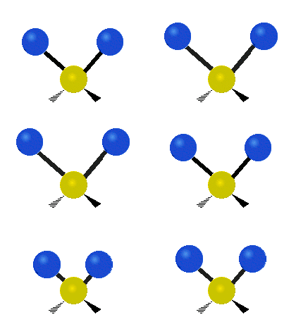
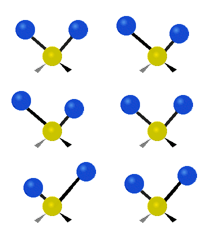
The atoms in a CH₂ group, commonly found in organic compounds, can vibrate in six different ways: symmetric and asymmetric stretching, scissoring, rocking, wagging and twisting as shown here:

Symmetrical stretching	Asymmetrical stretching	Scissoring (Bending)
Rocking	Wagging	Twisting

(These figures do not represent the "recoil" of the C atoms, which, though necessarily present to balance the overall movements of the molecule, are much smaller than the movements of the lighter H atoms).

Symmetry-adapted coordinates

Symmetry-adapted coordinates may be created by applying a projection operator to a set of internal coordinates.^[2] The projection operator is constructed with the aid of the character table of the molecular point group. For example, the four(un-normalised) C-H stretching coordinates of the molecule ethene are given by

where are the internal coordinates for stretching of each of the four C-H bonds.

Illustrations of symmetry-adapted coordinates for most small molecules can be found in Nakamoto.^[3]

Normal coordinates

The normal coordinates, denoted as Q, refer to the positions of atoms away from their equilibrium positions, with respect to a normal mode of vibration. Each normal mode is assigned a single normal coordinate, and so the normal coordinate refers to the "progress" along that normal mode at any given time. Formally, normal modes are determined by solving a secular determinant, and then the normal coordinates (over the normal modes) can be expressed as a summation over the cartesian coordinates (over the atom positions). The advantage of working in normal modes is that they diagonalize the matrix governing the molecular vibrations, so each normal mode is an independent molecular vibration, associated with its own spectrum of quantum mechanical states. If the molecule possesses symmetries, it will belong to a point group, and the normal modes will "transform as" an irreducible representation under that group. The normal modes can then be qualitatively determined by applying group theory and projecting the irreducible representation onto the cartesian coordinates. For example, when this treatment is applied to CO₂, it is found that the C=O stretches are not independent, but rather there is an O=C=O symmetric stretch and an O=C=O asymmetric stretch.

• symmetric stretching: the sum of the two C-O stretching coordinates; the two C-O bond lengths change by the same amount and the carbon atom is stationary. Q = q₁ + q₂
• asymmetric stretching: the difference of the two C-O stretching coordinates; one C-O bond length increases while the other decreases. Q = q₁ - q₂

When two or more normal coordinates belong to the same irreducible representation of the molecular point group (colloquially, have the same symmetry) there is "mixing" and the coefficients of the combination cannot be determined a priori. For example, in the linear molecule hydrogen cyanide, HCN, The two stretching vibrations are

1. principally C-H stretching with a little C-N stretching; Q₁ = q₁ + a q₂ (a << 1)
2. principally C-N stretching with a little C-H stretching; Q₂ = b q₁ + q₂ (b << 1)

The coefficients a and b are found by performing a full normal coordinate analysis by means of the Wilson GF method.^[4]

Newtonian mechanics

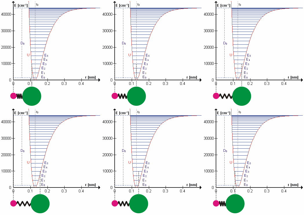
The HCl molecule as an anharmonic oscillator vibrating at energy level E₃. D₀ is dissociation energy here, r₀ bond length, U potential energy. Energy is expressed in wavenumbers. The hydrogen chloride molecule is attached to the coordinate system to show bond length changes on the curve.

Perhaps surprisingly, molecular vibrations can be treated using Newtonian mechanics to calculate the correct vibration frequencies. The basic assumption is that each vibration can be treated as though it corresponds to a spring. In the harmonic approximation the spring obeys Hooke's law: the force required to extend the spring is proportional to the extension. The proportionality constant is known as a force constant, k. The anharmonic oscillator is considered elsewhere.^[5]

By Newton’s second law of motion this force is also equal to a reduced mass, μ, times acceleration.

Since this is one and the same force the ordinary differential equation follows.

The solution to this equation of simple harmonic motion is

A is the maximum amplitude of the vibration coordinate Q. It remains to define the reduced mass, μ. In general, the reduced mass of a diatomic molecule, AB, is expressed in terms of the atomic masses, m_A and m_B, as

The use of the reduced mass ensures that the centre of mass of the molecule is not affected by the vibration. In the harmonic approximation the potential energy of the molecule is a quadratic function of the normal coordinate. It follows that the force-constant is equal to the second derivative of the potential energy.

When two or more normal vibrations have the same symmetry a full normal coordinate analysis must be performed (see GF method). The vibration frequencies,ν_i are obtained from the eigenvalues,λ_i, of the matrix product GF. G is a matrix of numbers derived from the masses of the atoms and the geometry of the molecule.^[4] F is a matrix derived from force-constant values. Details concerning the determination of the eigenvalues can be found in.^[6]

Quantum mechanics

In the harmonic approximation the potential energy is a quadratic function of the normal coordinates. Solving the Schrödinger wave equation, the energy states for each normal coordinate are given by

,

where n is a quantum number that can take values of 0, 1, 2 ... In molecular spectroscopy where several types of molecular energy are studied and several quantum numbers are used, this vibrational quantum number is often designated as v.^[7][8]

The difference in energy when n (or v) changes by 1 is therefore equal to , the product of the Planck constant and the vibration frequency derived using classical mechanics. For a transition from level n to level n+1 due to absorption of a photon, the frequency of the photon is equal to the classical vibration frequency (in the harmonic oscillator approximation).

See quantum harmonic oscillator for graphs of the first 5 wave functions, which allow certain selection rules to be formulated. For example, for a harmonic oscillator transitions are allowed only when the quantum number n changes by one,

but this does not apply to an anharmonic oscillator; the observation of overtones is only possible because vibrations are anharmonic. Another consequence of anharmonicity is that transitions such as between states n=2 and n=1 have slightly less energy than transitions between the ground state and first excited state. Such a transition gives rise to a hot band.

Intensities

In an infrared spectrum the intensity of an absorption band is proportional to the derivative of the molecular dipole moment with respect to the normal coordinate.^[9] The intensity of Raman bands depends on polarizability.

Uncertainty

From Wikipedia, the free encyclopedia

 

We are frequently presented with situations wherein a decision must be made when we are uncertain of exactly how to proceed.

Uncertainty is the situation which involves imperfect and / or unknown information. In other words it is a term used in subtly different ways in a number of fields, including insurance, philosophy, physics, statistics, economics, finance, psychology, sociology, engineering, metrology, and information science. It applies to predictions of future events, to physical measurements that are already made, or to the unknown. Uncertainty arises in partially observable and/or stochastic environments, as well as due to ignorance and/or indolence.^[1]

Concepts

Although the terms are used in various ways among the general public, many specialists in decision theory, statistics and other quantitative fields have defined uncertainty, risk, and their measurement as:

1. Uncertainty: The lack of certainty. A state of having limited knowledge where it is impossible to exactly describe the existing state, a future outcome, or more than one possible outcome.
2. Measurement of Uncertainty: A set of possible states or outcomes where probabilities are assigned to each possible state or outcome – this also includes the application of a probability density function to continuous variable
3. Risk: A state of uncertainty where some possible outcomes have an undesired effect or significant loss.
4. Measurement of Risk: A set of measured uncertainties where some possible outcomes are losses, and the magnitudes of those losses – this also includes loss functions over continuous variables.^[2]

Knightian uncertainty. In his seminal work Risk, Uncertainty, and Profit (1921), University of Chicago economist Frank Knight established the important distinction between risk and uncertainty:^[3]
There are other taxonomies of uncertainties and decisions that include a broader sense of uncertainty and how it should be approached from an ethics perspective:^[4]

A taxonomy of uncertainty

There are some things that you know to be true, and others that you know to be false; yet, despite this extensive knowledge that you have, there remain many things whose truth or falsity is not known to you. We say that you are uncertain about them. You are uncertain, to varying degrees, about everything in the future; much of the past is hidden from you; and there is a lot of the present about which you do not have full information. Uncertainty is everywhere and you cannot escape from it.

“

”

Dennis Lindley, Understanding Uncertainty (2006)

For example, if it is unknown whether or not it will rain tomorrow, then there is a state of uncertainty. If probabilities are applied to the possible outcomes using weather forecasts or even just a calibrated probability assessment, the uncertainty has been quantified. Suppose it is quantified as a 90% chance of sunshine. If there is a major, costly, outdoor event planned for tomorrow then there is a risk since there is a 10% chance of rain, and rain would be undesirable. Furthermore, if this is a business event and $100,000 would be lost if it rains, then the risk has been quantified(a 10% chance of losing $100,000). These situations can be made even more realistic by quantifying light rain vs. heavy rain, the cost of delays vs. outright cancellation, etc.

Some may represent the risk in this example as the "expected opportunity loss" (EOL) or the chance of the loss multiplied by the amount of the loss (10% × $100,000 = $10,000). That is useful if the organizer of the event is "risk neutral", which most people are not. Most would be willing to pay a premium to avoid the loss. An insurance company, for example, would compute an EOL as a minimum for any insurance coverage, then add onto that other operating costs and profit. Since many people are willing to buy insurance for many reasons, then clearly the EOL alone is not the perceived value of avoiding the risk.

Quantitative uses of the terms uncertainty and risk are fairly consistent from fields such as probability theory, actuarial science, and information theory. Some also create new terms without substantially changing the definitions of uncertainty or risk. For example, surprisal is a variation on uncertainty sometimes used in information theory. But outside of the more mathematical uses of the term, usage may vary widely. In cognitive psychology, uncertainty can be real, or just a matter of perception, such as expectations, threats, etc.

Vagueness or ambiguity are sometimes described as "second order uncertainty", where there is uncertainty even about the definitions of uncertain states or outcomes. The difference here is that this uncertainty is about the human definitions and concepts, not an objective fact of nature. It has been argued that ambiguity, however, is always avoidable while uncertainty (of the "first order" kind) is not necessarily avoidable.

Uncertainty may be purely a consequence of a lack of knowledge of obtainable facts. That is, there may be uncertainty about whether a new rocket design will work, but this uncertainty can be removed with further analysis and experimentation. At the subatomic level, however, uncertainty may be a fundamental and unavoidable property of the universe. In quantum mechanics, the Heisenberg Uncertainty Principle puts limits on how much an observer can ever know about the position and velocity of a particle. This may not just be ignorance of potentially obtainable facts but that there is no fact to be found. There is some controversy in physics as to whether such uncertainty is an irreducible property of nature or if there are "hidden variables" that would describe the state of a particle even more exactly than Heisenberg's uncertainty principle allows.

Measurements

In metrology, physics, and engineering, the uncertainty or margin of error of a measurement, when explicitly stated, is given by a range of values likely to enclose the true value. This may be denoted by error bars on a graph, or by the following notations:

• measured value ± uncertainty
• measured value +uncertainty
  −uncertainty
• measured value(uncertainty)

In the last notation, parentheses are the concise notation for the ± notation. For example applying 10 ¹⁄₂ meters in a scientific or engineering application, it could be written 7001105000000000000♠10.5 m or 7001105000000000000♠10.50 m, by convention meaning accurate to within one tenth of a meter, or one hundredth. The precision is symmetric around the last digit. In this case its half a tenth up and half a tenth down, so 10.5 means between 10.45 and 10.55. Thus it is understood that 10.5 means 7001105000000000000♠10.5±0.05, and 10.50 means 7001105000000000000♠10.50±0.005, also written 7001105000000000000♠10.5(0.5) and 7001105000000000000♠10.50(5). But if the accuracy is within two tenths, the uncertainty is ± one tenth, and it is required to be explicit: 7001105000000000000♠10.5±0.1 and 7001105000000000000♠10.50±0.01 or 7001105000000000000♠10.5(1)and 7001105000000000000♠10.50(1). The numbers in parenthesis apply to the numeral left of themselves, and are not part of that number, but part of a notation of uncertainty. They apply to the least significant digits. For instance, 7000100794000000000♠1.00794(7) stands for 7000100794000000000♠1.00794±0.00007, while 7000100794000000000♠1.00794(72) stands for 7000100794000000000♠1.00794±0.00072.^[5] This concise notation is used for example by IUPAC in stating the atomic mass of elements.
The middle notation is used when the error is not symmetrical about the value – for example 7000340000000000000♠3.4+0.3
−0.2. This can occur when using a logarithmic scale, for example.

Often, the uncertainty of a measurement is found by repeating the measurement enough times to get a good estimate of the standard deviation of the values. Then, any single value has an uncertainty equal to the standard deviation. However, if the values are averaged, then the mean measurement value has a much smaller uncertainty, equal to the standard error of the mean, which is the standard deviation divided by the square root of the number of measurements. This procedure neglects systematic errors, however.

When the uncertainty represents the standard error of the measurement, then about 68.3% of the time, the true value of the measured quantity falls within the stated uncertainty range. For example, it is likely that for 31.7% of the atomic mass values given on the list of elements by atomic mass, the true value lies outside of the stated range. If the width of the interval is doubled, then probably only 4.6% of the true values lie outside the doubled interval, and if the width is tripled, probably only 0.3% lie outside. These values follow from the properties of the normal distribution, and they apply only if the measurement process produces normally distributed errors. In that case, the quoted standard errors are easily converted to 68.3% ("one sigma"), 95.4% ("two sigma"), or 99.7% ("three sigma") confidence intervals.^{[citation needed]}

In this context, uncertainty depends on both the accuracy and precision of the measurement instrument. The lower the accuracy and precision of an instrument, the larger the measurement uncertainty is. Notice that precision is often determined as the standard deviation of the repeated measures of a given value, namely using the same method described above to assess measurement uncertainty. However, this method is correct only when the instrument is accurate. When it is inaccurate, the uncertainty is larger than the standard deviation of the repeated measures, and it appears evident that the uncertainty does not depend only on instrumental precision.

Uncertainty and the media

Uncertainty in science, and science in general, is often interpreted much differently in the public sphere than in the scientific community.^[6] This is due in part to the diversity of the public audience, and the tendency for scientists to misunderstand lay audiences and therefore not communicate ideas clearly and effectively.^[6] One example is explained by the information deficit model. Also, in the public realm, there are often many scientific voices giving input on a single topic.^[6] For example, depending on how an issue is reported in the public sphere, discrepancies between outcomes of multiple scientific studies due to methodological differences could be interpreted by the public as a lack of consensus in a situation where a consensus does in fact exist.^[6] This interpretation may have even been intentionally promoted, as scientific uncertainty may be managed to reach certain goals. For example, global warming contrarian activists took the advice of Frank Luntz to frame global warming as an issue of scientific uncertainty, which was a precursor to the conflict frame used by journalists when reporting the issue.^[7]

“Indeterminacy can be loosely said to apply to situations in which not all the parameters of the system and their interactions are fully known, whereas ignorance refers to situations in which it is not known what is not known”.^[8] These unknowns, indeterminacy and ignorance, that exist in science are often “transformed” into uncertainty when reported to the public in order to make issues more manageable, since scientific indeterminacy and ignorance are difficult concepts for scientists to convey without losing credibility.^[6] Conversely, uncertainty is often interpreted by the public as ignorance.^[9] The transformation of indeterminacy and ignorance into uncertainty may be related to the public’s misinterpretation of uncertainty as ignorance.

Journalists often either inflate uncertainty (making the science seem more uncertain than it really is) or downplay uncertainty (making the science seem more certain than it really is).^[10] One way that journalists inflate uncertainty is by describing new research that contradicts past research without providing context for the change^[10] Other times, journalists give scientists with minority views equal weight as scientists with majority views, without adequately describing or explaining the state of scientific consensus on the issue.^[10] In the same vein, journalists often give non-scientists the same amount of attention and importance as scientists.^[10]

Journalists may downplay uncertainty by eliminating “scientists’ carefully chosen tentative wording, and by losing these caveats the information is skewed and presented as more certain and conclusive than it really is”.^[10] Also, stories with a single source or without any context of previous research mean that the subject at hand is presented as more definitive and certain than it is in reality.^[10] There is often a “product over process” approach to science journalism that aids, too, in the downplaying of uncertainty.^[10] Finally, and most notably for this investigation, when science is framed by journalists as a triumphant quest, uncertainty is erroneously framed as “reducible and resolvable”.^[10]

Some media routines and organizational factors affect the overstatement of uncertainty; other media routines and organizational factors help inflate the certainty of an issue. Because the general public (in the United States) generally trusts scientists, when science stories are covered without alarm-raising cues from special interest organizations (religious groups, environmental organization, political factions, etc.) they are often covered in a business related sense, in an economic-development frame or a social progress frame.^[11] The nature of these frames is to downplay or eliminate uncertainty, so when economic and scientific promise are focused on early in the issue cycle, as has happened with coverage of plant biotechnology and nanotechnology in the United States, the matter in question seems more definitive and certain.^[11]

Sometimes, too, stockholders, owners, or advertising will pressure a media organization to promote the business aspects of a scientific issue, and therefore any uncertainty claims that may compromise the business interests are downplayed or eliminated.^[10]

Applications

• Investing in financial markets such as the stock market.
• Uncertainty or error is used in science and engineering notation. Numerical values should only be expressed to those digits that are physically meaningful, which are referred to as significant figures. Uncertainty is involved in every measurement, such as measuring a distance, a temperature, etc., the degree depending upon the instrument or technique used to make the measurement. Similarly, uncertainty is propagated through calculations so that the calculated value has some degree of uncertainty depending upon the uncertainties of the measured values and the equation used in the calculation.^[12]
• Uncertainty is designed into games, most notably in gambling, where chance is central to play.
• In scientific modelling, in which the prediction of future events should be understood to have a range of expected values.
• In physics, the Heisenberg uncertainty principle forms the basis of modern quantum mechanics.
• In weather forecasting it is now commonplace to include data on the degree of uncertainty in a weather forecast.
• Uncertainty is often an important factor in economics. According to economist Frank Knight, it is different from risk, where there is a specific probability assigned to each outcome (as when flipping a fair coin). Uncertainty involves a situation that has unknown probabilities, while the estimated probabilities of possible outcomes need not add to unity.
• In entrepreneurship: New products, services, firms and even markets are often created in the absence of probability estimates. According to entrepreneurship research, expert entrepreneurs predominantly use experience based heuristics called effectuation (as opposed to causality) to overcome uncertainty.
• In metrology, measurement uncertainty is a central concept quantifying the dispersion one may reasonably attribute to a measurement result. Such an uncertainty can also be referred to as a measurement error. In daily life, measurement uncertainty is often implicit ("He is 6 feet tall" give or take a few inches), while for any serious use an explicit statement of the measurement uncertainty is necessary. The expected measurement uncertainty of many measuring instruments (scales, oscilloscopes, force gages, rulers, thermometers, etc.) is often stated in the manufacturer's specification.
• Mobile phone radiation and health The most commonly used procedure for calculating measurement uncertainty is described in the "Guide to the Expression of Uncertainty in Measurement" (GUM) published by ISO. A derived work is for example the National Institute for Standards and Technology (NIST) Technical Note 1297, "Guidelines for Evaluating and Expressing the Uncertainty of NIST Measurement Results", and the Eurachem/Citac publication "Quantifying Uncertainty in Analytical Measurement". The uncertainty of the result of a measurement generally consists of several components. The components are regarded as random variables, and may be grouped into two categories according to the method used to estimate their numerical values:
  
  
  • Type A, those evaluated by statistical methods
  • Type B, those evaluated by other means, e.g., by assigning a probability distribution
  
  By propagating the variances of the components through a function relating the components to the measurement result, the combined measurement uncertainty is given as the square root of the resulting variance. The simplest form is the standard deviation of a repeated observation.
• Uncertainty has been a common theme in art, both as a thematic device (see, for example, the indecision of Hamlet), and as a quandary for the artist (such as Martin Creed's difficulty with deciding what artworks to make).
• Uncertainty assessment is significantly important for managing oil reservoirs where decisions are made based on uncertain models/outcomes. Predictions of oil and gas production from subsurface reservoirs are always uncertain.^[13][14]

Chimpanzee–human last common ancestor

From Wikipedia, the free encyclopedia

Chimpanzee–human last common ancestor Temporal range: 5.4–0 Ma PreЄ Є O S D C P T J K Pg N
Scientific classification
Kingdom:	Animalia
Phylum:	Chordata
Class:	Mammalia
Order:	Primates
Infraorder:	Simiiformes
Superfamily:	Hominoidea
Family:	Hominidae
Subfamily:	Homininae
Type species
Homo sapiens Linnaeus, 1758
Genera
Tribe Hominini Subtribe Panina Genus Pan Pan troglodytes Pan paniscus Subtribe Hominina Genus Homo Subtribe Australopithecina † Paranthropus † Australopithecus † Sahelanthropus † Orrorin † Ardipithecus † Kenyanthropus

The chimpanzee–human last common ancestor, or CHLCA, is the last species shared as a common ancestor by humans and chimpanzees; it represents the node point at which the line to genus Homo split from genus Pan. The last common ancestor of humans and chimps is estimated to have lived during the late Miocene, but possibly as late as Pliocene times—that is, more recent than 5.3 million years ago.

Speciation from Pan to Homo appears to have been a long, drawn-out process. After the "original" divergence(s), there were, according to Patterson (2006), periods of hybridization between population groups and a process of alternating divergence and hybridization that lasted over several millions of years.^[1] Sometime during the late Miocene or early Pliocene the earliest members of the human clade completed a final separation from the lineage of Pan—with dates estimated by several specialists ranging from 13 million ^[2] to as recent as 4 million years ago.^[3] The latter date and the argument for hybridization events are rejected by Wakeley^[4] (see current estimates regarding complex speciation).

Richard Wrangham (2001) argued that the CHLCA species was very similar to the common chimpanzee (Pan troglodytes)—so much so that it should be classified as a member of the Pan genus and be given the taxonomic name Pan prior.^[5] However, to date no fossil has been identified as a probable candidate for the CHLCA or the taxon Pan prior.

In human genetic studies, the CHLCA is useful as an anchor point for calculating single-nucleotide polymorphism (SNP) rates in human populations where chimpanzees are used as an outgroup, that is, as the extant species most genetically similar to Homo sapiens.

Time estimates

Historical studies

The earliest studies^{[year needed]} of apes suggested the CHLCA may have been as old as 25 million years; however, protein studies in the 1970s suggested the CHLCA was less than 8 million years in age. Genetic methods based on orangutan–human and gibbon–human LCA times were then used to estimate a chimpanzee–human LCA of 5 to 7 million years.

“	One no longer has the option of considering a fossil older than about eight million years as a hominid no matter what it looks like.	”
— V. Sarich, Background for man[6]

Some researchers tried to estimate the age of the CHLCA (T_CHLCA) using biopolymer structures that differ slightly between closely related animals. Among these researchers, Allan C. Wilson and Vincent Sarich were pioneers in the development of the molecular clock for humans. Working on protein sequences they eventually (1971) determined that apes were closer to humans than some paleontologists perceived based on the fossil record. ^[7] Later,^{[year needed]} Vincent Sarich concluded that the T_CHLCA was no greater than 8 million years in age, with a favored range between 4 and 6 million years before present.

This paradigmatic age has stuck with molecular anthropology until the late 1990s. Since the 1990s, the estimate has again been pushed towards more-remote times, because studies have found evidence for a slowing of the molecular clock as apes evolved from a common monkey-like ancestor with monkeys and humans evolved from a common ape-like ancestor with non-human apes.^[8]

Current estimates

Since the 1990s, the estimation of the T_CHLCA has become less certain, and there is genetic as well as paleontological support for increasing T_CHLCA beyond the 5 to 7 million years range accepted during the 1970s and 1980s. An estimate of T_CHLCA at 10 to 13 million years was proposed in 1998,^[9] and a range of 7 to 10 million years ago is assumed by White et a. (2009):

In effect, there is now no a priori reason to presume that human-chimpanzee split times are especially recent, and the fossil evidence is now fully compatible with older chimpanzee–human divergence dates [7 to 10 Ma...

— White et al. (2009), ^[10]

A source of confusion in determining the exact age of the Pan–Homo split is evidence of a more complex speciation process rather than a clean split between the two lineages. Different chromosomes appear to have split at different times, possibly over as much as a 4-million-year period, indicating a long and drawn out speciation process with large-scale hybridization events between the two emerging lineages as late as 6.3 to 5.4 million years ago according to Patterson et al. (2006).^[11] The assumption of late hybridization was in particular based on the similarity of the X chromosome in humans and chimpanzees, suggesting a divergence as late as some 4 million years ago. This conclusion was rejected as unwarranted by Wakeley (2008), who suggested alternative explanations, including selection pressure on the X chromosome in the populations ancestral to the CHLCA.^[12]

Complex speciation and incomplete lineage sorting of genetic sequences seem to also have happened in the split between the human lineage and that of the gorilla, indicating "messy" speciation is the rule rather than the exception in large primates.^[13][14] Such a scenario would explain why the divergence age between the Homo and Pan has varied with the chosen method and why a single point has so far been hard to track down.

Taxonomy

The taxon 'tribe Hominini' was proposed on basis of the idea that, regarding a trichotomy, the least similar species should be separated from the other two. Originally, this produced a separated Homo genus, which, predictably, was deemed the 'most different' among the three genera that includes Pan and Gorilla. However, later discoveries and analyses revealed that Pan and Homo are closer genetically than are Pan and Gorilla; thus, Pan was referred to the tribe Hominini with Homo.  Gorilla now became the separated genus and was referred to the new taxon 'tribe Gorillini' (see evolutionary tree here).

Mann and Weiss (1996), proposed that the tribe Hominini should encompass Pan as well as Homo, but grouped within separate subtribes.^[15] They would classify Homo and all bipedal apes to the subtribe Hominina and Pan to the subtribe Panina. (Wood (2010) discusses the different views of this taxonomy.)^[16] Richard Wrangham (2001) argued that the CHLCA species was very similar to chimpanzees (Pan troglodytes)—so much so that it should be classified as a member of the Pan genus and be given the taxonomic name Pan prior.^[5] To date, no fossil has been identified as a potential candidate for the CHLCA or the taxon Pan prior.

The 'human-side' descendants of the CHLCA species are specified as members of the tribe Hominini, that is, to the inclusion of the genus Homo and its closely related genus Australopithecus, but to the exclusion of the genus Pan—meaning all those human-related genera of tribe Hominini that arose after speciation from the line with Pan. Such grouping represents "the human clade" and its members are called "hominins".^[17] A "chimpanzee clade" was posited by Wood and Richard, who referred it to a 'Tribe Panini', which was envisioned from the family Hominidae being composed of a trifurcation of subfamilies.^[18]

Sahelanthropus tchadensis is an extinct hominid species with a morphology apparently as expected of the CHLCA; and it lived some 7 million years ago—which is very close to the time of the chimpanzee–human divergence. But it is unclear whether it should be classified as a member of the Hominini tribe, that is, a hominin, or as a direct ancestor of Homo and Pan and a potential candidate for the CHLCA species itself.

Few fossil specimens on the 'chimpanzee-side' of the split have been found; the first fossil chimpanzee, dating between 545 and 284 kyr (thousand years, radiometric), was discovered in Kenya's East African Rift Valley (McBrearty, 2005).^[19] All extinct genera listed in the taxobox are ancestral to Homo, or are offshoots of such. However, both Orrorin and Sahelanthropus existed around the time of the divergence, and so either one or both may be ancestral to both genera Homo and Pan.

Why Is Venus So Hot?

Surface temperatures of Venus are around 500 degrees C, some 485 degrees hotter than Earth (15 degrees C).  Although Venus has for decades been cited as a severe example of the "runaway greenhouse effect"  [http://www.esa.int/Our_Activities/Space_Science/Venus_Express/Greenhouse_effect_clouds_and_winds] for one example, there are problems with this theory [http://theendofthemystery.blogspot.gr/2010/11/venus-no-greenhouse-effect.html],
[http://www.perthnow.com.au/news/opinion/miranda-devine-perth-electrical-engineers-discovery-will-change-climate-change-debate/news-story/d1fe0f22a737e8d67e75a5014d0519c6], and [http://science.nasa.gov/science-news/science-at-nasa/2012/22mar_saber/]. In fact, it appears that it is Venus' dense atmosphere which accounts for most of the temperature diffence [https://en.wikipedia.org/wiki/Atmosphere_of_Venus-venus-atmosphere.html].

I was interested in using the Arrhenius equation to calculate how much greenhouse warming did contribute to Venus' lead-melting surface temperature. This equation can be summarized as

delta T = k * ln(C/C0).

In this case, I will use C = concentration of CO2 in Venus' atmosphere, and C0 as the concentration in Eath's atmosphere, and k as approximately 2.  Thus

2 * ln(90/0.0025) = 21 degrees C, or only 4% of the temperature difference between Earth and Venus!  This, it is important to add, does not include greenhouse cooling at the top of the atmosphere by CO2 deflecting incoming infrared, an effect that might reduce greenhouse heating by 80% or more.

Incidentally, if you want to know how hot Earth would get if the entire atmosphere were pure CO2 (2500 times greater), the same equation yields about a 10 degree rise (overlooking cooling and other effects of such high CO2 levels).

I said that the density of the Venusian atmosphere is responsible for (most of) its temperature.  There is a simple method of demonstrating this, although under the conditions we will consider there are some serious caveats to this method.  If you have ever studied gases in high school or college, you may have seen the equation

PV = nRT,

otherwise known as the ideal gas equation, where PV is the pressure times the volume of the gas, and nRT is the number of mols of gas (6.203E23 = molecules/mol), R is the ideal gas constant, and T is the temperature (in kelvins).  This is where one caveat comes in:  in principle there is no such thing as an "ideal gas", but most gases under Earthlike conditions come close enough for the equation to provide a reasonable approximation.  On Venus, however, things are trickier.

You probably know that when you compress a gas, its temperature rises, and vice versa.  (Bear in mind, you can compress with a constant pressure, which means P does not change.)  Starting with Earth's atmosphere (for it is closest to an ideal gas), we rearrange the equation above equation to:

T  = PV/nR, where we treat P/nR as a single constant, called K.  Then T(e) = K*V(e), and T(v) = K*V(v).  Then, again rearranging, we have T(v)/T(e) = V(v)/V(e) (K's cancel).  If you reduce the volume V(e) to the same density of V(v) -- a factor of about 90 -- then T(v) = 90*T(e).

Here, we run into our caveat, because the density of the Venusian gas is 90 times that of Earth's, and the temperature is about 2.67 times that of our planet (not 90).  Gas at such high density and temperature behaves in a highly non-ideal fasion; in fact, at the surface of Venus the carbon dioxide isn't even a gas anymore, but what's known as a "super critical" fluid, which absorbs much more heat than regular gases under Earth-like conditions.

Another factor comes into play here.  All gases, especially gases at high densities, are excellect heat insultors, due to conduction and convection.  I can think of no better example than our sun (or any star), in which a photon generated at the core takes thousands (or is it millions?) of years to reach the top of the atmosphere (the photosphere, the part we see) before zipping off into space at the speed of light.  Given that stars are almost entirely hydrogen and helium, non-greenhouse gases, that is clearly not the reason for this phenomenon.

Carboniferous

From Wikipedia, the free encyclopedia

Carboniferous Period 358.9–298.9 million years ago
Mean atmospheric O 2 content over period duration	ca. 32.5 vol %[1] (163 % of modern level)
Mean atmospheric CO 2 content over period duration	ca. 800 ppm[2] (3 times pre-industrial level)
Mean surface temperature over period duration	ca. 14 °C[3] (0 °C above modern level)
Sea level (above present day)	Falling from 120 m to present day level throughout Mississippian, then rising steadily to about 80 m at end of period[4]

The Carboniferous is a geologic period and system that extends from the end of the Devonian Period, at 358.9 ± 0.4 million years ago, to the beginning of the Permian Period, at 298.9 ± 0.15 Ma. The name Carboniferous means "coal-bearing" and derives from the Latin words carbō (“coal”) and ferō (“I bear, I carry”), and was coined by geologists William Conybeare and William Phillips in 1822.^[5] Based on a study of the British rock succession, it was the first of the modern 'system' names to be employed, and reflects the fact that many coal beds were formed globally during this time.^[6] The Carboniferous is often treated in North America as two geological periods, the earlier Mississippian and the later Pennsylvanian.^[7]

Terrestrial life was well established by the Carboniferous period.^[8] Amphibians were the dominant land vertebrates, of which one branch would eventually evolve into reptiles, the first fully terrestrial vertebrates. Arthropods were also very common, and many (such as Meganeura), were much larger than those of today. Vast swaths of forest covered the land, which would eventually be laid down and become the coal beds characteristic of the Carboniferous system. The atmospheric content of oxygen also reached their highest levels in history during the period, 35%^[9] compared with 21% today. This increased the atmospheric density by a third over today’s value.^[9] A minor marine and terrestrial extinction event occurred in the middle of the period, caused by a change in climate.^[10] The later half of the period experienced glaciations, low sea level, and mountain building as the continents collided to form Pangaea.

Subdivisions

In the United States the Carboniferous is usually broken into Mississippian (earlier) and Pennsylvanian (later) subperiods. The Mississippian is about twice as long as the Pennsylvanian, but due to the large thickness of coal bearing deposits with Pennsylvanian ages in Europe and North America, the two subperiods were long thought to have been more or less equal in duration.^[11] In Europe the Lower Carboniferous sub-system is known as the Dinantian, comprising the Tournaisian and Visean Series, dated at 362.5-332.9 Ma, and the Upper Carboniferous sub-system is known as the Silesian, comprising the Namurian, Westphalian, and Stephanian Series, dated at 332.9-290 Ma. The Silesian is roughly contemporaneous with the late Mississippian Serpukhovian plus the Pennsylvanian. In Britain the Dinantian is traditionally known as the Carboniferous Limestone, the Namurian as the Millstone Grit, and the Westphalian as the Coal Measures and Pennant Sandstone.
The faunal stages from youngest to oldest, together with some of their subdivisions, are:

Late Pennsylvanian: Gzhelian (most recent)

• Noginskian / Virgilian (part)

Late Pennsylvanian: Kasimovian

• Klazminskian
• Dorogomilovksian / Virgilian (part)
• Chamovnicheskian / Cantabrian / Missourian
• Krevyakinskian / Cantabrian / Missourian

Middle Pennsylvanian: Moscovian

• Myachkovskian / Bolsovian / Desmoinesian
• Podolskian / Desmoinesian
• Kashirskian / Atokan
• Vereiskian / Bolsovian / Atokan

Early Pennsylvanian: Bashkirian / Morrowan

• Melekesskian / Duckmantian
• Cheremshanskian / Langsettian
• Yeadonian
• Marsdenian
• Kinderscoutian

Late Mississippian: Serpukhovian

• Alportian
• Chokierian / Chesterian / Elvirian
• Arnsbergian / Elvirian
• Pendleian

Middle Mississippian: Visean

• Brigantian / St Genevieve / Gasperian / Chesterian
• Asbian / Meramecian
• Holkerian / Salem
• Arundian / Warsaw / Meramecian
• Chadian / Keokuk / Osagean (part) / Osage (part)

Early Mississippian: Tournaisian (oldest)

• Ivorian / (part) / Osage (part)
• Hastarian / Kinderhookian / Chouteau

Paleogeography

A global drop in sea level at the end of the Devonian reversed early in the Carboniferous; this created the widespread epicontinental seas and carbonate deposition of the Mississippian.^[12] There was also a drop in south polar temperatures; southern Gondwanaland was glaciated throughout the period, though it is uncertain if the ice sheets were a holdover from the Devonian or not.^[12] These conditions apparently had little effect in the deep tropics, where lush coal swamps flourished within 30 degrees of the northernmost glaciers.^[12]

Generalized geographic map of the United States in Middle Pennsylvanian time.

A mid-Carboniferous drop in sea level precipitated a major marine extinction, one that hit crinoids and ammonites especially hard.^[12] This sea level drop and the associated unconformity in North America separate the Mississippian subperiod from the Pennsylvanian subperiod.^[12] This happened about 318 million years ago, at the onset of the Permo-Carboniferous Glaciation.^{[citation needed]}

The Carboniferous was a time of active mountain-building, as the supercontinent Pangaea came together. The southern continents remained tied together in the supercontinent Gondwana, which collided with North America–Europe (Laurussia) along the present line of eastern North America. This continental collision resulted in the Hercynian orogeny in Europe, and the Alleghenian orogeny in North America; it also extended the newly uplifted Appalachians southwestward as the Ouachita Mountains.^[12] In the same time frame, much of present eastern Eurasian plate welded itself to Europe along the line of the Ural mountains. Most of the Mesozoic supercontinent of Pangea was now assembled, although North China (which would collide in the Latest Carboniferous), and South China continents were still separated from Laurasia. The Late Carboniferous Pangaea was shaped like an "O."

There were two major oceans in the Carboniferous—Panthalassa and Paleo-Tethys, which was inside the "O" in the Carboniferous Pangaea. Other minor oceans were shrinking and eventually closed - Rheic Ocean (closed by the assembly of South and North America), the small, shallow Ural Ocean (which was closed by the collision of Baltica and Siberia continents, creating the Ural Mountains) and Proto-Tethys Ocean (closed by North China collision with Siberia/Kazakhstania).

Climate and weather

Average global temperatures in the Early Carboniferous Period were high: approximately 20 °C (68 °F). However, cooling during the Middle Carboniferous reduced average global temperatures to about 12 °C (54 °F). Glaciations in Gondwana, triggered by Gondwana's southward movement, continued into the Permian and because of the lack of clear markers and breaks, the deposits of this glacial period are often referred to as Permo-Carboniferous in age.

The thicker atmosphere and stronger coriolis effect due to Earth's faster rotation (a day lasted for 22.4 hours in early Carboniferous) created significantly stronger winds than today.^[13]

The cooling and drying of the climate led to the Carboniferous Rainforest Collapse (CRC). Tropical rainforests fragmented and then were eventually devastated by climate change.^[10][14]

Rocks and coal

Lower Carboniferous marble in Big Cottonwood Canyon, Wasatch Mountains, Utah.

Carboniferous rocks in Europe and eastern North America largely consist of a repeated sequence of limestone, sandstone, shale and coal beds.^[15] In North America, the early Carboniferous is largely marine limestone, which accounts for the division of the Carboniferous into two periods in North American schemes. The Carboniferous coal beds provided much of the fuel for power generation during the Industrial Revolution and are still of great economic importance.

The large coal deposits of the Carboniferous may owe their existence primarily to two factors. The first of these is the appearance of wood tissue and bark-bearing trees. The evolution of the wood fiber lignin and the bark-sealing, waxy substance suberin variously opposed decay organisms so effectively that dead materials accumulated long enough to fossilise on a large scale. The second factor was the lower sea levels that occurred during the Carboniferous as compared to the preceding Devonian period. This promoted the development of extensive lowland swamps and forests in North America and Europe. Based on a genetic analysis of mushroom fungi, David Hibbett and colleagues proposed that large quantities of wood were buried during this period because animals and decomposing bacteria had not yet evolved enzymes that could effectively digest the resistant phenolic lignin polymers and waxy suberin polymers. They suggest that fungi that could break those substances down effectively only became dominant towards the end of the period, making subsequent coal formation much rarer.^[16][17][18]

The Carboniferous trees made extensive use of lignin. They had bark to wood ratios of 8 to 1, and even as high as 20 to 1. This compares to modern values less than 1 to 4. This bark, which must have been used as support as well as protection, probably had 38% to 58% lignin. Lignin is insoluble, too large to pass through cell walls, too heterogeneous for specific enzymes, and toxic, so that few organisms other than Basidiomycetes fungi can degrade it. To oxidize it requires an atmosphere of greater than 5% oxygen, or compounds such as peroxides. It can linger in soil for thousands of years and its toxic breakdown products inhibit decay of other substances.^[19] Probably the reason for its high percentages is protection from insect herbivory in a world containing very effective insect herbivores, but nothing remotely as effective as modern insectivores and probably many fewer poisons than currently. In any case coal measures could easily have made thick deposits on well drained soils as well as swamps. The extensive burial of biologically produced carbon led to an increase in oxygen levels in the atmosphere; estimates place the peak oxygen content as high as 35%, compared to 21% today.^[20] This oxygen level may have increased wildfire activity. It also may have promoted gigantism of insects and amphibians — creatures that have been constrained in size by respiratory systems that are limited in their physiological ability to transport and distribute oxygen at the lower atmospheric concentrations that have since been available.^[21]

In eastern North America, marine beds are more common in the older part of the period than the later part and are almost entirely absent by the late Carboniferous. More diverse geology existed elsewhere, of course. Marine life is especially rich in crinoids and other echinoderms. Brachiopods were abundant. Trilobites became quite uncommon. On land, large and diverse plant populations existed. Land vertebrates included large amphibians.

Life

Plants

Etching depicting some of the most significant plants of the Carboniferous.

Early Carboniferous land plants, some of which were preserved in coal balls, were very similar to those of the preceding Late Devonian, but new groups also appeared at this time.

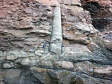
Ancient in situ lycopsid, probably Sigillaria, with attached stigmarian roots.

Base of a lycopsid showing connection with bifurcating stigmarian roots.

The main Early Carboniferous plants were the Equisetales (horse-tails), Sphenophyllales (scrambling plants), Lycopodiales (club mosses), Lepidodendrales (scale trees), Filicales (ferns), Medullosales (informally included in the "seed ferns", an artificial assemblage of a number of early gymnosperm groups) and the Cordaitales. These continued to dominate throughout the period, but during late Carboniferous, several other groups, Cycadophyta (cycads), the Callistophytales (another group of "seed ferns"), and the Voltziales (related to and sometimes included under the conifers), appeared.
The Carboniferous lycophytes of the order Lepidodendrales, which are cousins (but not ancestors) of the tiny club-moss of today, were huge trees with trunks 30 meters high and up to 1.5 meters in diameter. These included Lepidodendron (with its cone called Lepidostrobus), Anabathra, Lepidophloios and Sigillaria. The roots of several of these forms are known as Stigmaria. Unlike present day trees, their secondary growth took place in the cortex, which also provided stability, instead of the xylem.^[22] The Cladoxylopsids were large trees, that were ancestors of ferns, first arising in the Carboniferous.^[23]

The fronds of some Carboniferous ferns are almost identical with those of living species. Probably many species were epiphytic. Fossil ferns and "seed ferns" include Pecopteris, Cyclopteris, Neuropteris, Alethopteris, and Sphenopteris; Megaphyton and Caulopteris were tree ferns.

The Equisetales included the common giant form Calamites, with a trunk diameter of 30 to 60 cm (24 in) and a height of up to 20 m (66 ft). Sphenophyllum was a slender climbing plant with whorls of leaves, which was probably related both to the calamites and the lycopods.

Cordaites, a tall plant (6 to over 30 meters) with strap-like leaves, was related to the cycads and conifers; the catkin-like reproductive organs, which bore ovules/seeds, is called Cardiocarpus. These plants were thought to live in swamps and mangroves. True coniferous trees (Walchia, of the order Voltziales) appear later in the Carboniferous, and preferred higher drier ground.

Marine invertebrates

In the oceans the most important marine invertebrate groups are the Foraminifera, corals, Bryozoa, Ostracoda, brachiopods, ammonoids, hederelloids, microconchids and echinoderms (especially crinoids). For the first time foraminifera take a prominent part in the marine faunas. The large spindle-shaped genus Fusulina and its relatives were abundant in what is now Russia, China, Japan, North America; other important genera include Valvulina, Endothyra, Archaediscus, and Saccammina (the latter common in Britain and Belgium). Some Carboniferous genera are still extant.
The microscopic shells of radiolarians are found in cherts of this age in the Culm of Devon and Cornwall, and in Russia, Germany and elsewhere. Sponges are known from spicules and anchor ropes, and include various forms such as the Calcispongea Cotyliscus and Girtycoelia, the demosponge Chaetetes, and the genus of unusual colonial glass sponges Titusvillia.

Both reef-building and solitary corals diversify and flourish; these include both rugose (for example, Caninia, Corwenia, Neozaphrentis), heterocorals, and tabulate (for example, Chladochonus, Michelinia) forms. Conularids were well represented by Conularia

Bryozoa are abundant in some regions; the fenestellids including Fenestella, Polypora, and Archimedes, so named because it is in the shape of an Archimedean screw. Brachiopods are also abundant; they include productids, some of which (for example, Gigantoproductus) reached very large (for brachiopods) size and had very thick shells, while others like Chonetes were more conservative in form. Athyridids, spiriferids, rhynchonellids, and terebratulids are also very common. Inarticulate forms include Discina and Crania. Some species and genera had a very wide distribution with only minor variations.

Annelids such as Serpulites are common fossils in some horizons. Among the mollusca, the bivalves continue to increase in numbers and importance. Typical genera include Aviculopecten, Posidonomya, Nucula, Carbonicola, Edmondia, and Modiola Gastropods are also numerous, including the genera Murchisonia, Euomphalus, Naticopsis. Nautiloid cephalopods are represented by tightly coiled nautilids, with straight-shelled and curved-shelled forms becoming increasingly rare. Goniatite ammonoids are common.

Trilobites are rarer than in previous periods, on a steady trend towards extinction, represented only by the proetid group. Ostracoda, a class of crustaceans, were abundant as representatives of the meiobenthos; genera included Amphissites, Bairdia, Beyrichiopsis, Cavellina, Coryellina, Cribroconcha, Hollinella, Kirkbya, Knoxiella, and Libumella.

Amongst the echinoderms, the crinoids were the most numerous. Dense submarine thickets of long-stemmed crinoids appear to have flourished in shallow seas, and their remains were consolidated into thick beds of rock. Prominent genera include Cyathocrinus, Woodocrinus, and Actinocrinus. Echinoids such as Archaeocidaris and Palaeechinus were also present. The blastoids, which included the Pentreinitidae and Codasteridae and superficially resembled crinoids in the possession of long stalks attached to the seabed, attain their maximum development at this time.

• 

  Aviculopecten subcardiformis; a bivalve from the Logan Formation (Lower Carboniferous) of Wooster, Ohio (external mold).
• 

  Bivalves (Aviculopecten) and brachiopods (Syringothyris) in the Logan Formation (Lower Carboniferous) in Wooster, Ohio.
• 

  Syringothyris sp.; a spiriferid brachiopod from the Logan Formation (Lower Carboniferous) of Wooster, Ohio (internal mold).
• 

  Palaeophycus ichnosp.; a trace fossil from the Logan Formation (Lower Carboniferous) of Wooster, Ohio.
• 

  Crinoid calyx from the Lower Carboniferous of Ohio with a conical platyceratid gastropod (Palaeocapulus acutirostre) attached.
• 

  Conulariid from the Lower Carboniferous of Indiana.
• 

  Tabulate coral (a syringoporid); Boone Limestone (Lower Carboniferous) near Hiwasse, Arkansas.

Freshwater and lagoonal invertebrates

Freshwater Carboniferous invertebrates include various bivalve molluscs that lived in brackish or fresh water, such as Anthraconaia, Naiadites, and Carbonicola; diverse crustaceans such as Candona, Carbonita, Darwinula, Estheria, Acanthocaris, Dithyrocaris, and Anthrapalaemon.

The upper Carboniferous giant spider-like eurypterid Megarachne grew to legspans of 50 cm (20 in).

The Eurypterids were also diverse, and are represented by such genera as Anthraconectes, Megarachne (originally misinterpreted as a giant spider) and the specialised very large Hibbertopterus. Many of these were amphibious.

Frequently a temporary return of marine conditions resulted in marine or brackish water genera such as Lingula, Orbiculoidea, and Productus being found in the thin beds known as marine bands.

Terrestrial invertebrates

Fossil remains of air-breathing insects,^[24] myriapods and arachnids^[25] are known from the late Carboniferous, but so far not from the early Carboniferous.^[8] The first true priapulids appeared during this period. Their diversity when they do appear, however, shows that these arthropods were both well developed and numerous. Their large size can be attributed to the moistness of the environment (mostly swampy fern forests) and the fact that the oxygen concentration in the Earth's atmosphere in the Carboniferous was much higher than today.^[26] This required less effort for respiration and allowed arthropods to grow larger with the up to 2.6 metres long millipede-like Arthropleura being the largest known land invertebrate of all time. Among the insect groups are the huge predatory Protodonata (griffinflies), among which was Meganeura, a giant dragonfly-like insect and with a wingspan of ca. 75 cm (30 in) — the largest flying insect ever to roam the planet. Further groups are the Syntonopterodea (relatives of present-day mayflies), the abundant and often large sap-sucking Palaeodictyopteroidea, the diverse herbivorous Protorthoptera, and numerous basal Dictyoptera (ancestors of cockroaches).^[24] Many insects have been obtained from the coalfields of Saarbrücken and Commentry, and from the hollow trunks of fossil trees in Nova Scotia. Some British coalfields have yielded good specimens: Archaeoptitus, from the Derbyshire coalfield, had a spread of wing extending to more than 35 cm; some specimens (Brodia) still exhibit traces of brilliant wing colors. In the Nova Scotian tree trunks land snails (Archaeozonites, Dendropupa) have been found.

• 

  The late Carboniferous giant dragonfly-like insect Meganeura grew to wingspans of 75 cm (30 in).
• 

  The gigantic Pulmonoscorpius from the early Carboniferous reached a length of up to 70 cm (28 in).
• 

  Arthropleura, the largest land arthropod of all time.

Fish

Many fish inhabited the Carboniferous seas; predominantly Elasmobranchs (sharks and their relatives). These included some, like Psammodus, with crushing pavement-like teeth adapted for grinding the shells of brachiopods, crustaceans, and other marine organisms. Other sharks had piercing teeth, such as the Symmoriida; some, the petalodonts, had peculiar cycloid cutting teeth. Most of the sharks were marine, but the Xenacanthida invaded fresh waters of the coal swamps. Among the bony fish, the Palaeonisciformes found in coastal waters also appear to have migrated to rivers. Sarcopterygian fish were also prominent, and one group, the Rhizodonts, reached very large size.

Most species of Carboniferous marine fish have been described largely from teeth, fin spines and dermal ossicles, with smaller freshwater fish preserved whole.
Freshwater fish were abundant, and include the genera Ctenodus, Uronemus, Acanthodes, Cheirodus, and Gyracanthus.

Sharks (especially the Stethacanthids) underwent a major evolutionary radiation during the Carboniferous.^[27] It is believed that this evolutionary radiation occurred because the decline of the placoderms at the end of the Devonian period caused many environmental niches to become unoccupied and allowed new organisms to evolve and fill these niches.^[27] As a result of the evolutionary radiation carboniferous sharks assumed a wide variety of bizarre shapes including Stethacanthus which possessed a flat brush-like dorsal fin with a patch of denticles on its top.^[27] Stethacanthus' unusual fin may have been used in mating rituals.^[27]

• 

  Akmonistion of the shark order Symmoriida roamed the oceans of the early Carboniferous.
• 

  Falcatus was a Carboniferous shark, with a high degree of sexual dimorphism.

Tetrapods

Carboniferous amphibians were diverse and common by the middle of the period, more so than they are today; some were as long as 6 meters, and those fully terrestrial as adults had scaly skin.^[28] They included a number of basal tetrapod groups classified in early books under the Labyrinthodontia. These had long bodies, a head covered with bony plates and generally weak or undeveloped limbs. The largest were over 2 meters long. They were accompanied by an assemblage of smaller amphibians included under the Lepospondyli, often only about 15 cm (6 in) long. Some Carboniferous amphibians were aquatic and lived in rivers (Loxomma, Eogyrinus, Proterogyrinus); others may have been semi-aquatic (Ophiderpeton, Amphibamus, Hyloplesion) or terrestrial (Dendrerpeton, Tuditanus, Anthracosaurus).

The Carboniferous Rainforest Collapse slowed the evolution of amphibians who could not survive as well in the cooler, drier conditions. Reptiles, however prospered due to specific key adaptations.^[10] One of the greatest evolutionary innovations of the Carboniferous was the amniote egg, which allowed for the further exploitation of the land by certain tetrapods. These included the earliest sauropsid reptiles (Hylonomus), and the earliest known synapsid (Archaeothyris). These small lizard-like animals quickly gave rise to many descendants. The amniote egg allowed these ancestors of all later birds, mammals, and reptiles to reproduce on land by preventing the desiccation, or drying-out, of the embryo inside.

Reptiles underwent a major evolutionary radiation in response to the drier climate that preceded the rainforest collapse.^[10][29] By the end of the Carboniferous period, amniotes had already diversified into a number of groups, including protorothyridids, captorhinids, araeoscelids, and several families of pelycosaurs.

• 

  The amphibian-like Pederpes, the most primitive Mississippian tetrapod
• 

  Hylonomus, the earliest sauropsid reptile, appeared in the Pennsylvanian.
• 

  Petrolacosaurus, the first diapsid reptile known, lived during the late Carboniferous.
• 

  Archaeothyris was a very early mammal-like reptile and is the oldest undisputed synapsid known.

Fungi

Because plants and animals were growing in size and abundance in this time (for example, Lepidodendron), land fungi diversified further. Marine fungi still occupied the oceans. All modern classes of fungi were present in the Late Carboniferous (Pennsylvanian Epoch).^[30]

Extinction events

Romer's gap

The first 15 million years of the Carboniferous had very limited terrestrial fossils. This gap in the fossil record is called Romer's gap after the American palaentologist Alfred Romer. While it has long been debated whether the gap is a result of fossilisation or relates to an actual event, recent work indicates the gap period saw a drop in atmospheric oxygen levels, indicating some sort of ecological collapse.^[31] The gap saw the demise of the Devonian fish-like ichthyostegalian labyrinthodonts, and the rise of the more advanced temnospondyl and reptiliomorphan amphibians that so typify the Carboniferous terrestrial vertebrate fauna.

Carboniferous rainforest collapse

Before the end of the Carboniferous Period, an extinction event occurred. On land this event is referred to as the Carboniferous Rainforest Collapse (CRC).^[10] Vast tropical rainforests collapsed suddenly as the climate changed from hot and humid to cool and arid. This was likely caused by intense glaciation and a drop in sea levels.^[32]
The new climatic conditions were not favorable to the growth of rainforest and the animals within them. Rainforests shrank into isolated islands, surrounded by seasonally dry habitats. Towering lycopsid forests with a heterogeneous mixture of vegetation were replaced by much less diverse tree-fern dominated flora.

Amphibians, the dominant vertebrates at the time, fared poorly through this event with large losses in biodiversity; reptiles continued to diversify due to key adaptations that let them survive in the drier habitat, specifically the hard-shelled egg and scales, both of which retain water better than their amphibian counterparts.^[10]