Analytical skill

From Wikipedia, the free encyclopedia
https://en.wikipedia.org/wiki/Analytical_skill

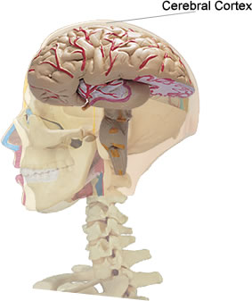
The cerebral cortex is responsible for analytical thinking in the human brain.

Analytical skill is the ability to deconstruct information into smaller categories in order to draw conclusions. Analytical skill consists of categories that include logical reasoning, critical thinking, communication, research, data analysis and creativity. Analytical skill is taught in contemporary education with the intention of fostering the appropriate practices for future professions. The professions that adopt analytical skill include educational institutions, public institutions, community organisations and industry.

Richards J. Heuer Jr. explained that

Thinking analytically is a skill like carpentry or driving a car. It can be taught, it can be learned, and it can improve with practice. But like many other skills, such as riding a bike, it is not learned by sitting in a classroom and being told how to do it. Analysts learn by doing.

In the article by Freed, the need for programs within the educational system to help students develop these skills is demonstrated. Workers "will need more than elementary basic skills to maintain the standard of living of their parents. They will have to think for a living, analyse problems and solutions, and work cooperatively in teams".

Logical Reasoning

Logical reasoning is a process consisting of inferences, where premises and hypotheses are formulated to arrive at a probable conclusion. It is a broad term covering three sub-classifications in deductive reasoning, inductive reasoning and abductive reasoning.

Deductive Reasoning

‘Deductive reasoning is a basic form of valid reasoning, commencing with a general statement or hypothesis, then examines the possibilities to reach a specific, logical conclusion’. This scientific method utilises deductions, to test hypotheses and theories, to predict if possible observations were correct.

A logical deductive reasoning sequence can be executed by establishing: an assumption, followed by another assumption and finally, conducting an inference. For example, ‘All men are mortal. Harold is a man. Therefore, Harold is mortal.’

For deductive reasoning to be upheld, the hypothesis must be correct, therefore, reinforcing the notion that the conclusion is logical and true. It is possible for deductive reasoning conclusions to be inaccurate or incorrect entirely, but the reasoning and premise is logical. For example, ‘All bald men are grandfathers. Harold is bald. Therefore, Harold is a grandfather.’ is a valid and logical conclusion but it is not true as the original assumption is incorrect. Deductive reasoning is an analytical skill used in many professions such as management, as the management team delegates tasks for day-to-day business operations.

Inductive Reasoning

Inductive reasoning compiles information and data to establish a general assumption that is suitable to the situation. Inductive reasoning commences with an assumption based on faithful data, leading to a generalised conclusion. For example, ‘All the swans I have seen are white. (Premise) Therefore all swans are white. (Conclusion)’. It is clear that the conclusion is incorrect, therefore, it is a weak argument. To strengthen the conclusion, it is made more probable, for example, ‘All the swans I have seen are white. (Premise) Therefore most swans are probably white (Conclusion)’. Inductive reasoning is an analytical skill common in many professions such as the corporate environment, where statistics and data are constantly analysed.

Doctor using abductive reasoning to diagnose a man with diabetes

The 6 types of inductive reasoning

1. Generalised: This manner utilises a premise on a sample set to extract a conclusion about a population.
2. Statistical: This is a method that utilises statistics based on a large and viable random sample set that is quantifiable to strengthen conclusions and observations.
3. Bayesian: This form adapts statistical reasoning to account for additional or new data.
4. Analogical: This is a method that records on the foundations of shared properties between two groups, leading to a conclusion that they are also likely to share further properties.
5. Predictive: This form of reasoning extrapolates a conclusion about the future based on a current or past sample.
6. Causal inference: This method of reasoning is formed around a causal link between the premise and the conclusion.

Abductive reasoning

Abductive reasoning commences with layered hypotheses, which may be insufficient with evidence, leading to a conclusion that is most likely explanatory for the problem. It is a form of reasoning where the conductor chooses a hypothesis that would best suit the given data. For example, when a patient is ill, the doctor gathers a hypothesis from the patient's symptoms, or other evidence, that they deem factual and appropriate. The doctor will then go through a list of possible illnesses and will attempt to assign the appropriate illness. Abductive reasoning is characterised by its lack of completeness, in evidence, explanation or both. This form of reasoning can be creative, intuitive and revolutionary due to its instinctive design.

Critical Thinking

Critical thinking is a skill used to interpret and explain the data given. It is the ability to think cautiously and rationally to resolve problems. This thinking is achieved by supporting conclusions without biases, having reliable evidence and reasoning, and using appropriate data and information. Critical thinking is an imperative skill as it underpins contemporary living in areas such as education and professional careers, but it is not restricted to a specific area.

Critical thinking is used to solve problems, calculate the likelihood, make decisions, and formulate inferences. Critical thinking requires examining information, reflective thinking, using appropriate skills, and confidence in the quality of the information given to come to a conclusion or plan. Critical thinking includes being willing to change if better information becomes available. As a critical thinker individuals do not accept assumptions without further questioning the reliability of it with further research and analysing the results found.

Developing Critical Thinking

Critical thinking can be developed through establishing personal beliefs and values. It is critical that individuals are able to query authoritative bodies: teachers, specialists, textbooks, books, newspapers, television etc. Querying these authorities allow critical thinking ability to be developed as the individual gains their own freedom and wisdom to think about reality and contemporary society, revering from autonomy.

Developing Critical Thinking through Probability Models

Critical thinking can be developed through probability models, where individuals adhere to a logical, conceptual understanding of mathematics and emphasise investigation, problem-solving, mathematical literacy and the use of mathematical discourse. The student actively constructs their knowledge and understanding, while teaching models function as a mediator by actively testing the student through querying, challenging and assigning investigation tasks, ultimately, allowing the student to think in deeper ways about various concepts, ideas and mathematical contexts.

Communication

Communication is a process where individuals transfer information from one another. It is a complex system consisting of a listener interpreting the information, understanding it and then transferring it. Communication as an analytical skill includes communicating with confidence, clarity, and sticking with the point you are trying to communicate. It consists of verbal and non-verbal communication. Communication is an imperative component of analytical skill as it allows the individual to develop relationships, contribute to group decisions, organisational communication, and influence media and culture.

Dr. Martin Luther King Jr. providing a speech to 250,000 people during the Civil Rights March in Washington D.C. exemplifies verbal communication

Verbal Communication

Verbal communication is interaction through words in linguistic form. Verbal communication consists of oral communication, written communication and sign language. It is an effective form of communication as the individuals sending and receiving the information are physically present, allowing immediate responses. In this form of communication, the sender uses words, spoken or written, to express the message to the individuals receiving the information.

Verbal communication is an essential analytical skill as it allows for the development of positive relationships among individuals. This positive relationship is attributed to the notion that verbal communication between individuals fosters a depth of understanding, empathy and versatility among them, providing each other with more attention. Verbal communication is a skill that is commonly used in professions such as the health sector, where healthcare workers are desired to possess strong interpersonal skills. Verbal communication has been linked to patient satisfaction. An effective strategy to improve verbal communication ability is through debating as is it fosters communication and critical thinking.

Non-verbal Communication

Non-verbal communication is commonly known as unspoken dialogue between individuals. It is a significant analytical skill as it allows individuals to distinguish true feelings, opinions and behaviours, as individuals are more likely to believe nonverbal cues as opposed to verbal expressions. Non-verbal communication is able to transcend communicational barriers such as race, ethnicity and sexual orientation.

Dancing is a common expressionist form of human non-verbal communication.

Statistical measures showcase that the true meaning behind all messages is 93% non-verbal and 7% verbal. Non-verbal communication is a critical analytical skill as it allows individuals to delve deeper into the meaning of messages. It allows individuals to analyse another person's perceptions, expressions and social beliefs. Individuals who excel in communicating and understanding non-verbal communication are able to analyse the interconnectedness of mutualism, social beliefs and expectations.

Communication Theories

A communication theory is an abstract understanding of how information is transferred from individuals. Many communication theories have been developed to foster and build upon the ongoing dynamic nature of how people communicate. Early models of communication were simple, such as Aristotle's model of communication, consisting of a speaker communicating a speech to an audience, leading to an effect. This is a basic form of communication that addresses communication as a linear concept where information is not being relayed back.

Modern theories for communication include Schramm's model where there are multiple individuals, each individual is encoding, interpreting and decoding the message, and messages are being transferred between one another. Schramm has included another factor in his model in experience i.e. expressing that each individual's experience influences their ability to interpret a message. Communication theories are constantly being developed to acclimatise to certain organisations or individuals. It is imperative for an individual to adopt a suitable communication theory for organisations to ensure that the organisation is able to function as desired. For example, traditional corporate hierarchy are commonly known to adopt a linear communicational model i.e. Aristotle's model of communication.

Research

Research is the construct of utilising tools and techniques to deconstruct and solve problems. While researching, it is important to distinguish what information is relevant to the data and avoiding excess, irrelevant data. Research involves the collection and analysis of information and data with the intention of founding new knowledge and/or deciphering a new understanding of existing data. Research ability is an analytical skill as it allows individuals to comprehend social implications. Research ability is valuable as it fosters transferable employment related skills. Research is primarily employed in academia and higher education, it is a profession pursued by many graduates, individuals intending to supervise or teach research students or those in pursuit of a PhD.

Research in Academia

In higher education, new research provides the most desired quality of evidence, if this is not available, then existing forms of evidence should be used. It is accepted that research provides the greatest form of knowledge, in the form of quantitative or qualitative data.

Research students are highly desired by various industries due to their dynamic mental capacity. Research students are commonly sought after due to their analysis and problem-solving ability, interpersonal and leadership skills, project management and organisation, research and information management and written and oral communication.

Data Analysis

Data analysis is a systematic method of cleaning, transforming and modelling statistical or logical techniques to describe and evaluate data. Using data analysis as an analytical skill means being able to examine large volumes of data and then identifying trends within the data. It is critical to be able to look at the data and determine what information is important and should be kept and what information is irrelevant and can be discarded. Data analysis includes finding different patterns within the information which allows you to narrow your research and come to a better conclusion. It is a tool to discover and decipher useful information for business decision-making. It is imperative in inferring information from data and adhering to a conclusion or decision from that data. Data analysis can stem from past or future data. Data analysis is an analytical skill, commonly adopted in business, as it allows organisations to become more efficient, internally and externally, solve complex problems and innovate.

Text Analysis

Text analysis is the discovery and understanding of valuable information in unstructured or large data. It is a method to transform raw data into business information, allowing for strategic business decisions by offering a method to extract and examine data, derive patterns and finally interpret the data.

Statistical Analysis

Statistical analysis involves the collection, analyses and presentation of data to decipher trends and patterns. It is common in research, industry and government to enhance the scientific aspects of the decision that needs to be made. It consists of descriptive analysis and inferential analysis.

Descriptive Analysis

Descriptive analysis provides information about a sample set that reflects the population by summarising relevant aspects of the dataset i.e. uncovering patterns. It displays the measures of central tendency and measures of spread, such as mean, deviation, proportion, frequency etc.

Inferential Analysis

Inferential analysis analyses a sample from complete data to compare the difference between treatment groups. Multiple conclusions are constructed by selecting different samples. Inferential analysis can provide evidence that, with a certain percentage of confidence, there is a relationship between two variables. It is adopted that the sample will be different to the population, thus, we further accept a degree of uncertainty.

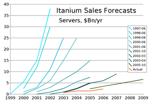
Example of sales forecasting, a form of predictive analysis

Diagnostic Analysis

Diagnostic analysis showcases the origin of the problem by finding the cause from the insight found in statistical analysis. This form of analysis is useful to identify behavioural patterns of data.

Predictive Analysis

Predictive analysis is an advanced form of analytics that forecasts future activity, behaviour, trends and patterns from new and historical data. Its accuracy is based on how much faithful data is present and the degree of inference that can be exploited from it.

Prescriptive Analysis

Prescriptive analytics provide firms with optimal recommendations to solve complex decisions. It is used in many industries, such as aviation to optimise schedule selection for airline crew.

Creativity

Areas of the brain that stimulated during actions of creativity

Creativity is important when it comes to solving different problems when presented. Creative thinking works best for problems that can have multiple solutions to solve the problem. It is also used when there seems to be no correct answer that applies to every situation, and is instead based from situation to situation. It includes being able to put the pieces of a problem together, as well as figure out pieces that may be missing. Then it includes brainstorming with all the pieces and deciding what pieces are important and what pieces can be discarded. The next step would be now analysing the pieces found to be of worth and importance and using those to come to a logical conclusion on how to best solve the problem. There can be multiple answers you come across to solve this problem. Many times creative thinking is referred to as right brain thinking. Creativity is an analytical skill as it allows individuals to utilise innovative methods to solve problems. Individuals that adopt this analytical skill are able to perceive problems from varying perspectives. This analytical skill is highly transferable among professions.

Energy flow (ecology)

From Wikipedia, the free encyclopedia

https://en.wikipedia.org/wiki/Energy_flow_(ecology)

A graphic representation of energy transfer between trophic layers in an ecosystem.

Energy flow is the flow of energy through living things within an ecosystem. All living organisms can be organized into producers and consumers, and those producers and consumers can further be organized into a food chain. Each of the levels within the food chain is a trophic level. In order to more efficiently show the quantity of organisms at each trophic level, these food chains are then organized into trophic pyramids. The arrows in the food chain show that the energy flow is unidirectional, with the head of an arrow indicating the direction of energy flow; energy is lost as heat at each step along the way.

The unidirectional flow of energy and the successive loss of energy as it travels up the food web are patterns in energy flow that are governed by thermodynamics, which is the theory of energy exchange between systems. Trophic dynamics relates to thermodynamics because it deals with the transfer and transformation of energy (originating externally from the sun via solar radiation) to and among organisms.

Energetics and the carbon cycle

The carbon cycle of a terrestrial ecosystem. Beginning with photosynthesis, water (blue) and carbon dioxide (white) from the air are taken in with solar energy (yellow), and are converted into plant energy (green). 100×10¹⁵ grams of carbon/year fixed by photosynthetic organisms, which is equivalent to 4×10¹⁸ kJ/yr = 4×10²¹ J/yr of free energy. Cellular respiration is the reverse reaction, wherein energy of plants is taken in and carbon dioxide and water are given off. The carbon dioxide and water produced can be recycled back into plants.

The first step in energetics is photosynthesis, where in water and carbon dioxide from the air are taken in with energy from the sun, and are converted into oxygen and glucose. Cellular respiration is the reverse reaction, wherein oxygen and sugar are taken in and release energy as they are converted back into carbon dioxide and water. The carbon dioxide and water produced by respiration can be recycled back into plants.

Energy loss can be measured either by efficiency (how much energy makes it to the next level), or by biomass (how much living material exists at those levels at one point in time, measured by standing crop). Of all the net primary productivity at the producer trophic level, in general only 10% goes to the next level, the primary consumers, then only 10% of that 10% goes on to the next trophic level, and so on up the food pyramid. Ecological efficiency may be anywhere from 5% to 20% depending on how efficient or inefficient that ecosystem is. This decrease in efficiency occurs because organisms need to perform cellular respiration to survive, and energy is lost as heat when cellular respiration is performed. That is also why there are fewer tertiary consumers than there are producers.

Primary production

Main article: Primary production

Fate of mangrove primary production

A producer is any organism that performs photosynthesis. Producers are important because they convert energy from the sun into a storable and usable chemical form of energy, glucose, as well as oxygen. The producers themselves can use the energy stored in glucose to perform cellular respiration. Or, if the producer is consumed by herbivores in the next trophic level, some of the energy is passed on up the pyramid. The glucose stored within producers serves as food for consumers, and so it is only through producers that consumers are able to access the sun’s energy. Some examples of primary producers are algae, mosses, and other plants such as grasses, trees, and shrubs.

Chemosynthetic bacteria perform a process similar to photosynthesis, but instead of energy from the sun they use energy stored in chemicals like hydrogen sulfide. This process, referred to as chemosynthesis, usually occurs deep in the ocean at hydrothermal vents that produce heat and chemicals such as hydrogen, hydrogen sulfide and methane. Chemosynthetic bacteria can use the energy in the bonds of the hydrogen sulfide and oxygen to convert carbon dioxide to glucose, releasing water and sulfur in the process. Organisms that consume the chemosynthetic bacteria can take in the glucose and use oxygen to perform cellular respiration, similar to herbivores consuming producers.

One of the factors that controls primary production is the amount of energy that enters the producer(s), which can be measured using productivity. Only one percent of solar energy enters the producer, the rest bounces off or moves through. Gross primary productivity is the amount of energy the producer actually gets. Generally, 60% of the energy that enters the producer goes to the producer’s own respiration. The net primary productivity is the amount that the plant retains after the amount that it used for cellular respiration is subtracted. Another factor controlling primary production is organic/inorganic nutrient levels in the water or soil that the producer is living in.

Secondary production

Secondary production is the use of energy stored in plants converted by consumers to their own biomass. Different ecosystems have different levels of consumers, all end with one top consumer. Most energy is stored in organic matter of plants, and as the consumers eat these plants they take up this energy. This energy in the herbivores and omnivores is then consumed by carnivores. There is also a large amount of energy that is in primary production and ends up being waste or litter, referred to as detritus. The detrital food chain includes a large amount of microbes, macroinvertebrates, meiofauna, fungi, and bacteria. These organisms are consumed by omnivores and carnivores and account for a large amount of secondary production. Secondary consumers can vary widely in how efficient they are in consuming. The efficiency of energy being passed on to consumers is estimated to be around 10%. Energy flow through consumers differs in aquatic and terrestrial environments.

In aquatic environments

Heterotrophs contribute to secondary production and it is dependent on primary productivity and the net primary products. Secondary production is the energy that herbivores and decomposers use and thus depends on primary productivity. Primarily herbivores and decomposers consume all the carbon from two main organic sources in aquatic ecosystems, autochthonous and allochthonous. Autochthonous carbon comes from within the ecosystem and includes aquatic plants, algae and phytoplankton. Allochthonous carbon from outside the ecosystem is mostly dead organic matter from the terrestrial ecosystem entering the water. In stream ecosystems, approximately 66% of annual energy input can be washed downstream. The remaining amount is consumed and lost as heat.

In terrestrial environments

Secondary production is often described in terms of trophic levels, and while this can be useful in explaining relationships it overemphasizes the rarer interactions. Consumers often feed at multiple trophic levels. Energy transferred above the third trophic level is relatively unimportant. The assimilation efficiency can be expressed by the amount of food the consumer has eaten, how much the consumer assimilates and what is expelled as feces or urine. While a portion of the energy is used for respiration, another portion of the energy goes towards biomass in the consumer. There are two major food chains: The primary food chain is the energy coming from autotrophs and passed on to the consumers; and the second major food chain is when carnivores eat the herbivores or decomposers that consume the autotrophic energy. Consumers are broken down into primary consumers, secondary consumers and tertiary consumers. Carnivores have a much higher assimilation of energy, about 80% and herbivores have a much lower efficiency of approximately 20 to 50%. Energy in a system can be affected by animal emigration/immigration. The movements of organisms are significant in terrestrial ecosystems. Energetic consumption by herbivores in terrestrial ecosystems has a low range of ~3-7%. The flow of energy is similar in many terrestrial environments. The fluctuation in the amount of net primary product consumed by herbivores is generally low. This is in large contrast to aquatic environments of lakes and ponds where grazers have a much higher consumption of around ~33%. Ectotherms and endotherms have very different assimilation efficiencies.

Detritivores

Detritivores consume organic material that is decomposing and are in turn consumed by carnivores. Predator productivity is correlated with prey productivity. This confirms that the primary productivity in ecosystems affects all productivity following.

Detritus is a large portion of organic material in ecosystems. Organic material in temperate forests is mostly made up of dead plants, approximately 62%.

In an aquatic ecosystem, leaf matter that falls into streams gets wet and begins to leech organic material. This happens rather quickly and will attract microbes and invertebrates. The leaves can be broken down into large pieces called coarse particulate organic matter (CPOM). The CPOM is rapidly colonized by microbes. Meiofauna is extremely important to secondary production in stream ecosystems. Microbes breaking down and colonizing this leaf matter are very important to the detritovores. The detritovores make the leaf matter more edible by releasing compounds from the tissues; it ultimately helps soften them. As leaves decay nitrogen will decrease since cellulose and lignin in the leaves is difficult to break down. Thus the colonizing microbes bring in nitrogen in order to aid in the decomposition. Leaf breakdown can depend on initial nitrogen content, season, and species of trees. The species of trees can have variation when their leaves fall. Thus the breakdown of leaves is happening at different times, which is called a mosaic of microbial populations.

Species effect and diversity in an ecosystem can be analyzed through their performance and efficiency. In addition, secondary production in streams can be influenced heavily by detritus that falls into the streams; production of benthic fauna biomass and abundance decreased an additional 47–50% during a study of litter removal and exclusion.

Energy flow across ecosystems

Research has demonstrated that primary producers fix carbon at similar rates across ecosystems. Once carbon has been introduced into a system as a viable source of energy, the mechanisms that govern the flow of energy to higher trophic levels vary across ecosystems. Among aquatic and terrestrial ecosystems, patterns have been identified that can account for this variation and have been divided into two main pathways of control: top-down and bottom-up. The acting mechanisms within each pathway ultimately regulate community and trophic level structure within an ecosystem to varying degrees. Bottom-up controls involve mechanisms that are based on resource quality and availability, which control primary productivity and the subsequent flow of energy and biomass to higher trophic levels. Top-down controls involve mechanisms that are based on consumption by consumers. These mechanisms control the rate of energy transfer from one trophic level to another as herbivores or predators feed on lower trophic levels.

Aquatic vs terrestrial ecosystems

Much variation in the flow of energy is found within each type of ecosystem, creating a challenge in identifying variation between ecosystem types. In a general sense, the flow of energy is a function of primary productivity with temperature, water availability, and light availability. For example, among aquatic ecosystems, higher rates of production are usually found in large rivers and shallow lakes than in deep lakes and clear headwater streams. Among terrestrial ecosystems, marshes, swamps, and tropical rainforests have the highest primary production rates, whereas tundra and alpine ecosystems have the lowest. The relationships between primary production and environmental conditions have helped account for variation within ecosystem types, allowing ecologists to demonstrate that energy flows more efficiently through aquatic ecosystems than terrestrial ecosystems due to the various bottom-up and top-down controls in play.

Bottom-up

The strength of bottom-up controls on energy flow are determined by the nutritional quality, size, and growth rates of primary producers in an ecosystem. Photosynthetic material is typically rich in nitrogen (N) and phosphorus (P) and supplements the high herbivore demand for N and P across all ecosystems. Aquatic primary production is dominated by small, single-celled phytoplankton that are mostly composed of photosynthetic material, providing an efficient source of these nutrients for herbivores. In contrast, multi-cellular terrestrial plants contain many large supporting cellulose structures of high carbon but low nutrient value. Because of this structural difference, aquatic primary producers have less biomass per photosynthetic tissue stored within the aquatic ecosystem than in the forests and grasslands of terrestrial ecosystems. This low biomass relative to photosynthetic material in aquatic ecosystems allows for a more efficient turnover rate compared to terrestrial ecosystems. As phytoplankton are consumed by herbivores, their enhanced growth and reproduction rates sufficiently replace lost biomass and, in conjunction with their nutrient dense quality, support greater secondary production.

Additional factors impacting primary production includes inputs of N and P, which occurs at a greater magnitude in aquatic ecosystems. These nutrients are important in stimulating plant growth and, when passed to higher trophic levels, stimulate consumer biomass and growth rate. If either of these nutrients are in short supply, they can limit overall primary production. Within lakes, P tends to be the greater limiting nutrient while both N and P limit primary production in rivers. Due to these limiting effects, nutrient inputs can potentially alleviate the limitations on net primary production of an aquatic ecosystem. Allochthonous material washed into an aquatic ecosystem introduces N and P as well as energy in the form of carbon molecules that are readily taken up by primary producers. Greater inputs and increased nutrient concentrations support greater net primary production rates, which in turn supports greater secondary production.

Top-down

Top-down mechanisms exert greater control on aquatic primary producers due to the roll of consumers within an aquatic food web. Among consumers, herbivores can mediate the impacts of trophic cascades by bridging the flow of energy from primary producers to predators in higher trophic levels. Across ecosystems, there is a consistent association between herbivore growth and producer nutritional quality. However, in aquatic ecosystems, primary producers are consumed by herbivores at a rate four times greater than in terrestrial ecosystems. Although this topic is highly debated, researchers have attributed the distinction in herbivore control to several theories, including producer to consumer size ratios and herbivore selectivity.

A freshwater food web demonstrating the size differences between each trophic level. Primary producers tend to be small algal cells. Herbivores tend to be small macro-invertebrates. Predators tend to be larger fish.

Modeling of top-down controls on primary producers suggests that the greatest control on the flow of energy occurs when the size ratio of consumer to primary producer is the highest. The size distribution of organisms found within a single trophic level in aquatic systems is much narrower than that of terrestrial systems. On land, the consumer size ranges from smaller than the plant it consumes, such as an insect, to significantly larger, such as an ungulate, while in aquatic systems, consumer body size within a trophic level varies much less and is strongly correlated with trophic position. As a result, the size difference between producers and consumers is consistently larger in aquatic environments than on land, resulting in stronger herbivore control over aquatic primary producers.

Herbivores can potentially control the fate of organic matter as it is cycled through the food web. Herbivores tend to select nutritious plants while avoiding plants with structural defense mechanisms. Like support structures, defense structures are composed of nutrient poor, high carbon cellulose. Access to nutritious food sources enhances herbivore metabolism and energy demands, leading to greater removal of primary producers. In aquatic ecosystems, phytoplankton are highly nutritious and generally lack defense mechanisms. This results in greater top-down control because consumed plant matter is quickly released back into the system as labile organic waste. In terrestrial ecosystems, primary producers are less nutritionally dense and are more likely to contain defense structures. Because herbivores prefer nutritionally dense plants and avoid plants or plant parts with defense structures, a greater amount of plant matter is left unconsumed within the ecosystem. Herbivore avoidance of low-quality plant matter may be why terrestrial systems exhibit weaker top-down control on the flow of energy.

Online machine learning

From Wikipedia, the free encyclopedia

https://en.wikipedia.org/wiki/Online_machine_learning

In computer science, online machine learning is a method of machine learning in which data becomes available in a sequential order and is used to update the best predictor for future data at each step, as opposed to batch learning techniques which generate the best predictor by learning on the entire training data set at once. Online learning is a common technique used in areas of machine learning where it is computationally infeasible to train over the entire dataset, requiring the need of out-of-core algorithms. It is also used in situations where it is necessary for the algorithm to dynamically adapt to new patterns in the data, or when the data itself is generated as a function of time, e.g., prediction of prices in the financial international markets. Online learning algorithms may be prone to catastrophic interference, a problem that can be addressed by incremental learning approaches.

Introduction

In the setting of supervised learning, a function of ${\displaystyle f:X\to Y}$ is to be learned, where ${\displaystyle X}$ is thought of as a space of inputs and ${\displaystyle Y}$ as a space of outputs, that predicts well on instances that are drawn from a joint probability distribution ${\displaystyle p(x,y)}$ on ${\displaystyle X\times Y}$. In reality, the learner never knows the true distribution ${\displaystyle p(x,y)}$ over instances. Instead, the learner usually has access to a training set of examples ${\displaystyle (x_1,y_1),\dots ,(x_n,y_n)}$. In this setting, the loss function is given as ${\displaystyle V:Y\times Y\to \mathbb{R}}$, such that ${\displaystyle V(f(x),y)}$ measures the difference between the predicted value ${\displaystyle f(x)}$ and the true value ${\displaystyle y}$. The ideal goal is to select a function ${\displaystyle f\in \mathcal{H}}$, where ${\displaystyle \mathcal{H}}$ is a space of functions called a hypothesis space, so that some notion of total loss is minimized. Depending on the type of model (statistical or adversarial), one can devise different notions of loss, which lead to different learning algorithms.

Statistical view of online learning

In statistical learning models, the training sample ${\displaystyle (x_i,y_i)}$ are assumed to have been drawn from the true distribution ${\displaystyle p(x,y)}$ and the objective is to minimize the expected "risk" $${\displaystyle I[f]=\mathbb{E}[V(f(x),y)]=\int V(f(x),y)dp(x,y).}$$ A common paradigm in this situation is to estimate a function ${\displaystyle \hat{f}}$ through empirical risk minimization or regularized empirical risk minimization (usually Tikhonov regularization). The choice of loss function here gives rise to several well-known learning algorithms such as regularized least squares and support vector machines. A purely online model in this category would learn based on just the new input ${\displaystyle (x_{t+1},y_{t+1})}$, the current best predictor ${\displaystyle f_t}$ and some extra stored information (which is usually expected to have storage requirements independent of training data size). For many formulations, for example nonlinear kernel methods, true online learning is not possible, though a form of hybrid online learning with recursive algorithms can be used where ${\displaystyle f_{t+1}}$ is permitted to depend on ${\displaystyle f_t}$ and all previous data points ${\displaystyle (x_1,y_1),\dots ,(x_t,y_t)}$. In this case, the space requirements are no longer guaranteed to be constant since it requires storing all previous data points, but the solution may take less time to compute with the addition of a new data point, as compared to batch learning techniques.

A common strategy to overcome the above issues is to learn using mini-batches, which process a small batch of ${\displaystyle b\ge 1}$ data points at a time, this can be considered as pseudo-online learning for ${\displaystyle b}$ much smaller than the total number of training points. Mini-batch techniques are used with repeated passing over the training data to obtain optimized out-of-core versions of machine learning algorithms, for example, stochastic gradient descent. When combined with backpropagation, this is currently the de facto training method for training artificial neural networks.

Example: linear least squares

Main article: Linear least squares (mathematics)

The simple example of linear least squares is used to explain a variety of ideas in online learning. The ideas are general enough to be applied to other settings, for example, with other convex loss functions.

Batch learning

Consider the setting of supervised learning with ${\displaystyle f}$ being a linear function to be learned: $${\displaystyle f(x_j)=⟨w,x_j⟩=w\cdot x_j}$$ where ${\displaystyle x_j\in {\mathbb{R}}^d}$ is a vector of inputs (data points) and ${\displaystyle w\in {\mathbb{R}}^d}$ is a linear filter vector. The goal is to compute the filter vector ${\displaystyle w}$. To this end, a square loss function $${\displaystyle V(f(x_j),y_j)=(f(x_j)-y_j{)}^2=(⟨w,x_j⟩-y_j{)}^2}$$ is used to compute the vector ${\displaystyle w}$ that minimizes the empirical loss $${\displaystyle I_n[w]=\sum _{j=1}^{n}V(⟨w,x_j⟩,y_j)=\sum _{j=1}^n(x_j^{\mathsf{T}}w-y_j{)}^2}$$ where $${\displaystyle y_j\in \mathbb{R}.}$$

Let ${\displaystyle X}$ be the ${\displaystyle i\times d}$ data matrix and ${\displaystyle y\in {\mathbb{R}}^i}$ is the column vector of target values after the arrival of the first ${\displaystyle i}$ data points. Assuming that the covariance matrix ${\displaystyle {\mathrm{\Sigma }}_i=X^{\mathsf{T}}X}$ is invertible (otherwise it is preferential to proceed in a similar fashion with Tikhonov regularization), the best solution ${\displaystyle f^{\ast }(x)=⟨w^{\ast },x⟩}$ to the linear least squares problem is given by $${\displaystyle w^{\ast }=(X^{\mathsf{T}}X{)}^{-1}{X}^{\mathsf{T}}y={\mathrm{\Sigma }}_i^{-1}\sum _{j=1}^i{x}_j{y}_j.}$$

Now, calculating the covariance matrix ${\displaystyle {\mathrm{\Sigma }}_i=\sum _{j=1}^i{x}_j{x}_j^{\mathsf{T}}}$ takes time ${\displaystyle O(i{d}^2)}$, inverting the ${\displaystyle d\times d}$ matrix takes time ${\displaystyle O(d^3)}$, while the rest of the multiplication takes time ${\displaystyle O(d^2)}$, giving a total time of ${\displaystyle O(i{d}^2+d^3)}$. When there are ${\displaystyle n}$ total points in the dataset, to recompute the solution after the arrival of every datapoint ${\displaystyle i=1,\dots ,n}$, the naive approach will have a total complexity ${\displaystyle O(n^2{d}^2+n{d}^3)}$. Note that when storing the matrix ${\displaystyle {\mathrm{\Sigma }}_i}$, then updating it at each step needs only adding ${\displaystyle x_{i+1}{x}_{i+1}^{\mathsf{T}}}$, which takes ${\displaystyle O(d^2)}$ time, reducing the total time to ${\displaystyle O(n{d}^2+n{d}^3)=O(n{d}^3)}$, but with an additional storage space of ${\displaystyle O(d^2)}$ to store ${\displaystyle {\mathrm{\Sigma }}_i}$.

Online learning: recursive least squares

The recursive least squares (RLS) algorithm considers an online approach to the least squares problem. It can be shown that by initialising ${\displaystyle w_0=0\in {\mathbb{R}}^d}$ and ${\displaystyle {\mathrm{\Gamma }}_0=I\in {\mathbb{R}}^{d\times d}}$, the solution of the linear least squares problem given in the previous section can be computed by the following iteration: $${\displaystyle {\mathrm{\Gamma }}_i={\mathrm{\Gamma }}_{i-1}-\frac{{\mathrm{\Gamma }}_{i-1}{x}_i{x}_i^{\mathsf{T}}{\mathrm{\Gamma }}_{i-1}}{1+x_i^{\mathsf{T}}{\mathrm{\Gamma }}_{i-1}{x}_i}}$$ $${\displaystyle w_i=w_{i-1}-{\mathrm{\Gamma }}_i{x}_i\left(x_i^{\mathsf{T}}{w}_{i-1}-y_i\right)}$$ The above iteration algorithm can be proved using induction on ${\displaystyle i}$. The proof also shows that ${\displaystyle {\mathrm{\Gamma }}_i={\mathrm{\Sigma }}_i^{-1}}$. One can look at RLS also in the context of adaptive filters (see RLS).

The complexity for ${\displaystyle n}$ steps of this algorithm is ${\displaystyle O(n{d}^2)}$, which is an order of magnitude faster than the corresponding batch learning complexity. The storage requirements at every step ${\displaystyle i}$ here are to store the matrix ${\displaystyle {\mathrm{\Gamma }}_i}$, which is constant at ${\displaystyle O(d^2)}$. For the case when ${\displaystyle {\mathrm{\Sigma }}_i}$ is not invertible, consider the regularised version of the problem loss function ${\displaystyle \sum _{j=1}^n{\left(x_j^{\mathsf{T}}w-y_j\right)}^2+\lambda {\Vert w\Vert }_2^2}$. Then, it's easy to show that the same algorithm works with ${\displaystyle {\mathrm{\Gamma }}_0=(I+\lambda I{)}^{-1}}$, and the iterations proceed to give ${\displaystyle {\mathrm{\Gamma }}_i=({\mathrm{\Sigma }}_i+\lambda I{)}^{-1}}$.

Stochastic gradient descent

Main article: Stochastic gradient descent

When this $${\displaystyle w_i=w_{i-1}-{\mathrm{\Gamma }}_i{x}_i\left(x_i^{\mathsf{T}}{w}_{i-1}-y_i\right)}$$ is replaced by $${\displaystyle w_i=w_{i-1}-{\gamma }_i{x}_i\left(x_i^{\mathsf{T}}{w}_{i-1}-y_i\right)=w_{i-1}-{\gamma }_i\mathrm{\nabla }V(⟨w_{i-1},x_i⟩,y_i)}$$ or ${\displaystyle {\mathrm{\Gamma }}_i\in {\mathbb{R}}^{d\times d}}$ by ${\displaystyle {\gamma }_i\in \mathbb{R}}$, this becomes the stochastic gradient descent algorithm. In this case, the complexity for ${\displaystyle n}$ steps of this algorithm reduces to ${\displaystyle O(nd)}$. The storage requirements at every step ${\displaystyle i}$ are constant at ${\displaystyle O(d)}$.

However, the stepsize ${\displaystyle {\gamma }_i}$ needs to be chosen carefully to solve the expected risk minimization problem, as detailed above. By choosing a decaying step size ${\displaystyle {\gamma }_i\approx \frac{1}{\sqrt{i}},}$ one can prove the convergence of the average iterate ${\overline{w}}_n=\frac{1}{n}\sum _{i=1}^n{w}_i$. This setting is a special case of stochastic optimization, a well known problem in optimization.

Incremental stochastic gradient descent

In practice, one can perform multiple stochastic gradient passes (also called cycles or epochs) over the data. The algorithm thus obtained is called incremental gradient method and corresponds to an iteration $${\displaystyle w_i=w_{i-1}-{\gamma }_i\mathrm{\nabla }V(⟨w_{i-1},x_{t_i}⟩,y_{t_i})}$$ The main difference with the stochastic gradient method is that here a sequence ${\displaystyle t_i}$ is chosen to decide which training point is visited in the ${\displaystyle i}$-th step. Such a sequence can be stochastic or deterministic. The number of iterations is then decoupled to the number of points (each point can be considered more than once). The incremental gradient method can be shown to provide a minimizer to the empirical risk. Incremental techniques can be advantageous when considering objective functions made up of a sum of many terms e.g. an empirical error corresponding to a very large dataset.

Kernel methods

See also: Kernel method

Kernels can be used to extend the above algorithms to non-parametric models (or models where the parameters form an infinite dimensional space). The corresponding procedure will no longer be truly online and instead involve storing all the data points, but is still faster than the brute force method. This discussion is restricted to the case of the square loss, though it can be extended to any convex loss. It can be shown by an easy induction  that if ${\displaystyle X_i}$ is the data matrix and ${\displaystyle w_i}$ is the output after ${\displaystyle i}$ steps of the SGD algorithm, then, $${\displaystyle w_i=X_i^{\mathsf{T}}{c}_i}$$ where ${\displaystyle c_i=((c_i{)}_1,(c_i{)}_2,...,(c_i{)}_i)\in {\mathbb{R}}^i}$ and the sequence ${\displaystyle c_i}$ satisfies the recursion: $${\displaystyle c_0=0}$$ $${\displaystyle (c_i{)}_j=(c_{i-1}{)}_j,j=1,2,...,i-1}$$ and $${\displaystyle (c_i{)}_i={\gamma }_i(y_i-\sum _{j=1}^{i-1}(c_{i-1}{)}_j⟨x_j,x_i⟩)}$$ Notice that here ${\displaystyle ⟨x_j,x_i⟩}$ is just the standard Kernel on ${\displaystyle {\mathbb{R}}^d}$, and the predictor is of the form $${\displaystyle f_i(x)=⟨w_{i-1},x⟩=\sum _{j=1}^{i-1}(c_{i-1}{)}_j⟨x_j,x⟩.}$$

Now, if a general kernel ${\displaystyle K}$ is introduced instead and let the predictor be $${\displaystyle f_i(x)=\sum _{j=1}^{i-1}(c_{i-1}{)}_{j}K(x_j,x)}$$ then the same proof will also show that predictor minimising the least squares loss is obtained by changing the above recursion to $${\displaystyle (c_i{)}_i={\gamma }_i(y_i-\sum _{j=1}^{i-1}(c_{i-1}{)}_{j}K(x_j,x_i))}$$ The above expression requires storing all the data for updating ${\displaystyle c_i}$. The total time complexity for the recursion when evaluating for the ${\displaystyle n}$-th datapoint is ${\displaystyle O(n^{2}dk)}$, where ${\displaystyle k}$ is the cost of evaluating the kernel on a single pair of points. Thus, the use of the kernel has allowed the movement from a finite dimensional parameter space ${\displaystyle w_i\in {\mathbb{R}}^d}$ to a possibly infinite dimensional feature represented by a kernel ${\displaystyle K}$ by instead performing the recursion on the space of parameters ${\displaystyle c_i\in {\mathbb{R}}^i}$, whose dimension is the same as the size of the training dataset. In general, this is a consequence of the representer theorem.

Online convex optimization

Online convex optimization (OCO)  is a general framework for decision making which leverages convex optimization to allow for efficient algorithms. The framework is that of repeated game playing as follows:

For ${\displaystyle t=1,2,...,T}$

• Learner receives input ${\displaystyle x_t}$
• Learner outputs ${\displaystyle w_t}$ from a fixed convex set ${\displaystyle S}$
• Nature sends back a convex loss function ${\displaystyle v_t:S\to \mathbb{R}}$.
• Learner suffers loss ${\displaystyle v_t(w_t)}$ and updates its model

The goal is to minimize regret, or the difference between cumulative loss and the loss of the best fixed point ${\displaystyle u\in S}$ in hindsight. As an example, consider the case of online least squares linear regression. Here, the weight vectors come from the convex set ${\displaystyle S={\mathbb{R}}^d}$, and nature sends back the convex loss function ${\displaystyle v_t(w)=(⟨w,x_t⟩-y_t{)}^2}$. Note here that ${\displaystyle y_t}$ is implicitly sent with ${\displaystyle v_t}$.

Some online prediction problems however cannot fit in the framework of OCO. For example, in online classification, the prediction domain and the loss functions are not convex. In such scenarios, two simple techniques for convexification are used: randomisation and surrogate loss functions.

Some simple online convex optimisation algorithms are:

Follow the leader (FTL)

The simplest learning rule to try is to select (at the current step) the hypothesis that has the least loss over all past rounds. This algorithm is called Follow the leader, and round ${\displaystyle t}$ is simply given by: $${\displaystyle w_t=\underset{w\in S}{\mathrm{a}\mathrm{r}\mathrm{g}\mathrm{m}\mathrm{i}\mathrm{n}}\sum _{i=1}^{t-1}{v}_i(w)}$$ This method can thus be looked as a greedy algorithm. For the case of online quadratic optimization (where the loss function is ${\displaystyle v_t(w)={\Vert w-x_t\Vert }_2^2}$), one can show a regret bound that grows as ${\displaystyle \log (T)}$. However, similar bounds cannot be obtained for the FTL algorithm for other important families of models like online linear optimization. To do so, one modifies FTL by adding regularisation.

Follow the regularised leader (FTRL)

This is a natural modification of FTL that is used to stabilise the FTL solutions and obtain better regret bounds. A regularisation function ${\displaystyle R:S\to \mathbb{R}}$ is chosen and learning performed in round t as follows: $${\displaystyle w_t=\underset{w\in S}{\mathrm{a}\mathrm{r}\mathrm{g}\mathrm{m}\mathrm{i}\mathrm{n}}\sum _{i=1}^{t-1}{v}_i(w)+R(w)}$$ As a special example, consider the case of online linear optimisation i.e. where nature sends back loss functions of the form ${\displaystyle v_t(w)=⟨w,z_t⟩}$. Also, let ${\displaystyle S={\mathbb{R}}^d}$. Suppose the regularisation function $R(w)=\frac{1}{2\eta }{\Vert w\Vert }_2^2$ is chosen for some positive number ${\displaystyle \eta }$. Then, one can show that the regret minimising iteration becomes $${\displaystyle w_{t+1}=-\eta \sum _{i=1}^t{z}_i=w_t-\eta z_t}$$ Note that this can be rewritten as ${\displaystyle w_{t+1}=w_t-\eta \mathrm{\nabla }{v}_t(w_t)}$, which looks exactly like online gradient descent.

If S is instead some convex subspace of ${\displaystyle {\mathbb{R}}^d}$, S would need to be projected onto, leading to the modified update rule $${\displaystyle w_{t+1}={\mathrm{\Pi }}_S(-\eta \sum _{i=1}^t{z}_i)={\mathrm{\Pi }}_S(\eta {\theta }_{t+1})}$$ This algorithm is known as lazy projection, as the vector ${\displaystyle {\theta }_{t+1}}$ accumulates the gradients. It is also known as Nesterov's dual averaging algorithm. In this scenario of linear loss functions and quadratic regularisation, the regret is bounded by ${\displaystyle O(\sqrt{T})}$, and thus the average regret goes to 0 as desired.

Online subgradient descent (OSD)

See also: Subgradient method

The above proved a regret bound for linear loss functions ${\displaystyle v_t(w)=⟨w,z_t⟩}$. To generalise the algorithm to any convex loss function, the subgradient ${\displaystyle \mathrm{\partial }{v}_t(w_t)}$ of ${\displaystyle v_t}$ is used as a linear approximation to ${\displaystyle v_t}$ near ${\displaystyle w_t}$, leading to the online subgradient descent algorithm:

Initialise parameter ${\displaystyle \eta ,w_1=0}$

For ${\displaystyle t=1,2,...,T}$

• Predict using ${\displaystyle w_t}$, receive ${\displaystyle f_t}$ from nature.
• Choose ${\displaystyle z_t\in \mathrm{\partial }{v}_t(w_t)}$
• If ${\displaystyle S={\mathbb{R}}^d}$, update as ${\displaystyle w_{t+1}=w_t-\eta z_t}$
• If ${\displaystyle S\subset {\mathbb{R}}^d}$, project cumulative gradients onto ${\displaystyle S}$ i.e. ${\displaystyle w_{t+1}={\mathrm{\Pi }}_S(\eta {\theta }_{t+1}),{\theta }_{t+1}={\theta }_t+z_t}$

One can use the OSD algorithm to derive ${\displaystyle O(\sqrt{T})}$ regret bounds for the online version of SVM's for classification, which use the hinge loss${\displaystyle v_t(w)=max\{0,1-y_t(w\cdot x_t)\}}$

Other algorithms

Quadratically regularised FTRL algorithms lead to lazily projected gradient algorithms as described above. To use the above for arbitrary convex functions and regularisers, one uses online mirror descent. The optimal regularization in hindsight can be derived for linear loss functions, this leads to the AdaGrad algorithm. For the Euclidean regularisation, one can show a regret bound of ${\displaystyle O(\sqrt{T})}$, which can be improved further to a ${\displaystyle O(\log T)}$ for strongly convex and exp-concave loss functions.

Continual learning

Continual learning means constantly improving the learned model by processing continuous streams of information. Continual learning capabilities are essential for software systems and autonomous agents interacting in an ever changing real world. However, continual learning is a challenge for machine learning and neural network models since the continual acquisition of incrementally available information from non-stationary data distributions generally leads to catastrophic forgetting.

Interpretations of online learning

The paradigm of online learning has different interpretations depending on the choice of the learning model, each of which has distinct implications about the predictive quality of the sequence of functions ${\displaystyle f_1,f_2,\dots ,f_n}$. The prototypical stochastic gradient descent algorithm is used for this discussion. As noted above, its recursion is given by $${\displaystyle w_t=w_{t-1}-{\gamma }_t\mathrm{\nabla }V(⟨w_{t-1},x_t⟩,y_t)}$$

The first interpretation consider the stochastic gradient descent method as applied to the problem of minimizing the expected risk ${\displaystyle I[w]}$ defined above. Indeed, in the case of an infinite stream of data, since the examples ${\displaystyle (x_1,y_1),(x_2,y_2),\dots }$ are assumed to be drawn i.i.d. from the distribution ${\displaystyle p(x,y)}$, the sequence of gradients of ${\displaystyle V(\cdot ,\cdot )}$ in the above iteration are an i.i.d. sample of stochastic estimates of the gradient of the expected risk ${\displaystyle I[w]}$ and therefore one can apply complexity results for the stochastic gradient descent method to bound the deviation ${\displaystyle I[w_t]-I[w^{\ast }]}$, where ${\displaystyle w^{\ast }}$ is the minimizer of ${\displaystyle I[w]}$. This interpretation is also valid in the case of a finite training set; although with multiple passes through the data the gradients are no longer independent, still complexity results can be obtained in special cases.

The second interpretation applies to the case of a finite training set and considers the SGD algorithm as an instance of incremental gradient descent method. In this case, one instead looks at the empirical risk: $${\displaystyle I_n[w]=\frac{1}{n}\sum _{i=1}^{n}V(⟨w,x_i⟩,y_i).}$$ Since the gradients of ${\displaystyle V(\cdot ,\cdot )}$ in the incremental gradient descent iterations are also stochastic estimates of the gradient of ${\displaystyle I_n[w]}$, this interpretation is also related to the stochastic gradient descent method, but applied to minimize the empirical risk as opposed to the expected risk. Since this interpretation concerns the empirical risk and not the expected risk, multiple passes through the data are readily allowed and actually lead to tighter bounds on the deviations ${\displaystyle I_n[w_t]-I_n[w_n^{\ast }]}$, where ${\displaystyle w_n^{\ast }}$ is the minimizer of ${\displaystyle I_n[w]}$.

Implementations

• Vowpal Wabbit: Open-source fast out-of-core online learning system which is notable for supporting a number of machine learning reductions, importance weighting and a selection of different loss functions and optimisation algorithms. It uses the hashing trick for bounding the size of the set of features independent of the amount of training data.
• scikit-learn: Provides out-of-core implementations of algorithms for
  • Classification: Perceptron, SGD classifier, Naive bayes classifier.
  • Regression: SGD Regressor, Passive Aggressive regressor.
  • Clustering: Mini-batch k-means.
  • Feature extraction: Mini-batch dictionary learning, Incremental PCA.