In chemistry, a double bond is a covalent bond between two atoms involving four bonding electrons as opposed to two in a single bond. Double bonds occur most commonly between two carbon atoms, for example in alkenes. Many double bonds exist between two different elements: for example, in a carbonyl group between a carbon atom and an oxygen atom. Other common double bonds are found in azo compounds (N=N), imines (C=N), and sulfoxides (S=O). In a skeletal formula, a double bond is drawn as two parallel lines (=) between the two connected atoms; typographically, the equals sign is used for this. Double bonds were introduced in chemical notation by Russian chemist Alexander Butlerov.
Double bonds involving carbon are stronger and shorter than single bonds. The bond order
is two. Double bonds are also electron-rich, which makes them
potentially more reactive in the presence of a strong electron acceptor
(as in addition reactions of the halogens).
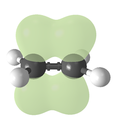
The type of bonding can be explained in terms of orbital hybridisation. In ethylene each carbon atom has three sp2 orbitals and one p-orbital. The three sp2
orbitals lie in a plane with ~120° angles. The p-orbital is
perpendicular to this plane. When the carbon atoms approach each other,
two of the sp2 orbitals overlap to form a sigma bond. At the same time, the two p-orbitals approach (again in the same plane) and together they form a pi bond.
For maximum overlap, the p-orbitals have to remain parallel, and,
therefore, rotation around the central bond is not possible. This
property gives rise to cis-trans isomerism. Double bonds are shorter than single bonds because p-orbital overlap is maximized.
2 sp2 orbitals (total of 3 such orbitals) approach to form a sp2-sp2 sigma bond
Two p-orbitals overlap to form a pi-bond in a plane parallel to the sigma plane
With 133 pm, the ethylene C=Cbond length is shorter than the C−C length in ethane with 154 pm. The double bond is also stronger, 636 kJmol−1 versus 368 kJ mol−1 but not twice as much as the pi-bond is weaker than the sigma bond due to less effective pi-overlap.
In an alternative representation, the double bond results from two overlapping sp3 orbitals as in a bent bond.[3]
Variations
In
molecules with alternating double bonds and single bonds, p-orbital
overlap can exist over multiple atoms in a chain, giving rise to a conjugated system. Conjugation can be found in systems such as dienes and enones. In cyclic molecules, conjugation can lead to aromaticity. In cumulenes, two double bonds are adjacent.
Double bonded compounds, alkene homologs, R2E=ER2 are now known for all of the heavier group 14
elements. Unlike the alkenes these compounds are not planar but adopt
twisted and/or trans bent structures. These effects become more
pronounced for the heavier elements. The distannene (Me3Si)2CHSn=SnCH(SiMe3)2
has a tin-tin bond length just a little shorter than a single bond, a
trans bent structure with pyramidal coordination at each tin atom, and
readily dissociates in solution to form (Me3Si)2CHSn:
(stannanediyl, a carbene analog). The bonding comprises two weak donor
acceptor bonds, the lone pair on each tin atom overlapping with the
empty p orbital on the other.
In contrast, in disilenes each silicon atom has planar coordination
but the substituents are twisted so that the molecule as a whole is not
planar. In diplumbenes the Pb=Pb bond length can be longer than that of
many corresponding single bonds
Plumbenes and stannenes generally dissociate in solution into monomers
with bond enthalpies that are just a fraction of the corresponding
single bonds. Some double bonds plumbenes and stannenes are similar in
strength to hydrogen bonds. The Carter-Goddard-Malrieu-Trinquier model can be used to predict the nature of the bonding.
The
horseshoe shaped ribonuclease inhibitor (shown as wireframe) forms a
protein–protein interaction with the ribonuclease protein. The contacts
between the two proteins are shown as coloured patches.
Protein–protein interactions (PPIs) are physical contacts of high specificity established between two or more protein molecules as a result of biochemical events steered by interactions that include electrostatic forces, hydrogen bonding and the hydrophobic effect.
Many are physical contacts with molecular associations between chains
that occur in a cell or in a living organism in a specific biomolecular
context.
Proteins rarely act alone as their functions tend to be regulated. Many molecular processes within a cell are carried out by molecular machines
that are built from numerous protein components organized by their
PPIs. These physiological interactions make up the so-called interactomics of the organism, while aberrant PPIs are the basis of multiple aggregation-related diseases, such as Creutzfeldt–Jakob and Alzheimer's diseases.
In many metabolic reactions, a protein that acts as an electron carrier binds to an enzyme that acts as its reductase. After it receives an electron, it dissociates and then binds to the next enzyme that acts as its oxidase
(i.e. an acceptor of the electron). These interactions between proteins
are dependent on highly specific binding between proteins to ensure
efficient electron transfer. Examples: mitochondrial oxidative
phosphorylation chain system components cytochrome c-reductase / cytochrome c / cytochrome c oxidase; microsomal and mitochondrial P450 systems.
In the case of the mitochondrial P450 systems, the specific residues involved in the binding of the electron transfer protein adrenodoxin
to its reductase were identified as two basic Arg residues on the
surface of the reductase and two acidic Asp residues on the adrenodoxin.
More recent work on the phylogeny of the reductase has shown that these
residues involved in protein–protein interactions have been conserved
throughout the evolution of this enzyme.
The activity of the cell is regulated by extracellular signals.
Signal propagation inside and/or along the interior of cells depends on
PPIs between the various signaling molecules. The recruitment of
signaling pathways through PPIs is called signal transduction and plays a fundamental role in many biological processes and in many diseases including Parkinson's disease and cancer.
To describe the types of protein–protein interactions (PPIs) it is
important to consider that proteins can interact in a "transient" way
(to produce some specific effect in a short time, like signal
transduction) or to interact with other proteins in a "stable" way to
form complexes that become molecular machines within the living systems.
A protein complex assembly can result in the formation of homo-oligomeric or hetero-oligomeric complexes.
In addition to the conventional complexes, as enzyme-inhibitor and
antibody-antigen, interactions can also be established between
domain-domain and domain-peptide. Another important distinction to
identify protein–protein interactions is the way they have been
determined, since there are techniques that measure direct physical
interactions between protein pairs, named “binary” methods, while there
are other techniques that measure physical interactions among groups of
proteins, without pairwise determination of protein partners, named
“co-complex” methods.
Homo-oligomers vs. hetero-oligomers
Homo-oligomers are macromolecular complexes constituted by only one type of protein subunit. Protein subunits assembly is guided by the establishment of non-covalent interactions in the quaternary structure of the protein. Disruption of homo-oligomers in order to return to the initial individual monomers often requires denaturation of the complex. Several enzymes, carrier proteins,
scaffolding proteins, and transcriptional regulatory factors carry out
their functions as homo-oligomers.
Distinct protein subunits interact in hetero-oligomers, which are
essential to control several cellular functions. The importance of the
communication between heterologous proteins is even more evident during
cell signaling events and such interactions are only possible due to
structural domains within the proteins (as described below).
Stable interactions vs. transient interactions
Stable
interactions involve proteins that interact for a long time, taking
part of permanent complexes as subunits, in order to carry out
functional roles. These are usually the case of homo-oligomers (e.g. cytochrome c), and some hetero-oligomeric proteins, as the subunits of ATPase. On the other hand, a protein may interact briefly and in a reversible manner with other proteins in only certain cellular contexts – cell type, cell cycle stage, external factors, presence of other binding proteins, etc. – as it happens with most of the proteins involved in biochemical cascades. These are called transient interactions. For example, some G protein–coupled receptors only transiently bind to Gi/o proteins when they are activated by extracellular ligands, while some Gq-coupled receptors, such as muscarinic receptor M3, pre-couple with Gq proteins prior to the receptor-ligand binding. Interactions between intrinsically disordered protein regions to globular protein domains (i.e. MoRFs) are transient interactions.
Water molecules play a significant role in the interactions between proteins.
The crystal structures of complexes, obtained at high resolution from
different but homologous proteins, have shown that some interface water
molecules are conserved between homologous complexes. The majority of
the interface water molecules make hydrogen bonds with both partners of
each complex. Some interface amino acid residues or atomic groups of one
protein partner engage in both direct and water mediated interactions
with the other protein partner. Doubly indirect interactions, mediated
by two water molecules, are more numerous in the homologous complexes of
low affinity.
Carefully conducted mutagenesis experiments, e.g. changing a tyrosine
residue into a phenylalanine, have shown that water mediated
interactions can contribute to the energy of interaction. Thus, water molecules may facilitate the interactions and cross-recognitions between proteins.
The molecular structures of many protein complexes have been unlocked by the technique of X-ray crystallography. The first structure to be solved by this method was that of sperm whalemyoglobin by Sir John Cowdery Kendrew.
In this technique the angles and intensities of a beam of X-rays
diffracted by crystalline atoms are detected in a film, thus producing a
three-dimensional picture of the density of electrons within the
crystal.
Later, nuclear magnetic resonance
also started to be applied with the aim of unravelling the molecular
structure of protein complexes. One of the first examples was the
structure of calmodulin-binding domains bound to calmodulin.
This technique is based on the study of magnetic properties of atomic
nuclei, thus determining physical and chemical properties of the
correspondent atoms or the molecules. Nuclear magnetic resonance is
advantageous for characterizing weak PPIs.
SH2 domains are structurally composed by three-stranded twisted
beta sheet sandwiched flanked by two alpha-helices. The existence of a
deep binding pocket with high affinity for phosphotyrosine, but not for phosphoserine or phosphothreonine, is essential for the recognition of tyrosine phosphorylated proteins, mainly autophosphorylated growth factor receptors. Growth factor receptor binding proteins and phospholipase Cγ are examples of proteins that have SH2 domains.
Structurally, SH3 domains are constituted by a beta barrel
formed by two orthogonal beta sheets and three anti-parallel beta
strands. These domains recognize proline enriched sequences, as polyproline type II helical structure (PXXP motifs) in cell signaling proteins like protein tyrosine kinases and the growth factor receptor bound protein 2 (Grb2).
LIM domains were initially identified in three homeodomain transcription factors (lin11, is11, and mec3). In addition to this homeodomain proteins
and other proteins involved in development, LIM domains have also been
identified in non-homeodomain proteins with relevant roles in cellular differentiation, association with cytoskeleton and senescence. These domains contain a tandem cysteine-rich Zn2+-finger motif and embrace the consensus sequence CX2CX16-23HX2CX2CX2CX16-21CX2C/H/D. LIM domains bind to PDZ domains, bHLH transcription factors, and other LIM domains.
SAM domains are composed by five helices forming a compact package with a conserved hydrophobic core. These domains, which can be found in the Eph receptor and the stromal interaction molecule (STIM) for example, bind to non-SAM domain-containing proteins and they also appear to have the ability to bind RNA.
PDZ domains were first identified in three guanylate kinases:
PSD-95, DlgA and ZO-1. These domains recognize carboxy-terminal
tri-peptide motifs (S/TXV), other PDZ domains or LIM domains and bind them through a short peptide sequence that has a C-terminal
hydrophobic residue. Some of the proteins identified as having PDZ
domains are scaffolding proteins or seem to be involved in ion receptor
assembling and receptor-enzyme complexes formation.
FERM domains contain basic residues capable of binding PtdIns(4,5)P2. Talin and focal adhesion kinase (FAK) are two of the proteins that present FERM domains.
The
study of the molecular structure can give fine details about the
interface that enables the interaction between proteins. When
characterizing PPI interfaces it is important to take into account the
type of complex.
Parameters evaluated include size (measured in absolute dimensions Å2 or in solvent-accessible surface area (SASA)),
shape, complementarity between surfaces, residue interface
propensities, hydrophobicity, segmentation and secondary structure, and
conformational changes on complex formation.
The great majority of PPI interfaces reflects the composition of
protein surfaces, rather than the protein cores, in spite of being
frequently enriched in hydrophobic residues, particularly in aromatic
residues. PPI interfaces are dynamic and frequently planar, although they can be globular and protruding as well. Based on three structures – insulin dimer, trypsin-pancreatic trypsin inhibitor complex, and oxyhaemoglobin – Cyrus Chothia and Joel Janin found that between 1,130 and 1,720 Å2 of surface area was removed from contact with water indicating that hydrophobicity is a major factor of stabilization of PPIs. Later studies refined the buried surface area of the majority of interactions to 1,600±350 Å2. However, much larger interaction interfaces were also observed and were associated with significant changes in conformation of one of the interaction partners. PPIs interfaces exhibit both shape and electrostatic complementarity.
Regulation
Protein concentration, which in turn are affected by expression levels and degradation rates;
Protein affinity for proteins or other binding ligands;
This system was firstly described in 1989 by Fields and Song using Saccharomyces cerevisiae as biological model. Yeast two hybrid allows the identification of pairwise PPIs (binary method) in vivo,
in which the two proteins are tested for biophysically direct
interaction. The Y2H is based on the functional reconstitution of the
yeast transcription factor Gal4 and subsequent activation of a selective
reporter such as His3. To test two proteins for interaction, two
protein expression constructs are made: one protein (X) is fused to the
Gal4 DNA-binding domain (DB) and a second protein (Y) is fused to the
Gal4 activation domain (AD). In the assay, yeast cells are transformed
with these constructs. Transcription of reporter genes does not occur
unless bait (DB-X) and prey (AD-Y) interact with each other and form a
functional Gal4 transcription factor. Thus, the interaction between
proteins can be inferred by the presence of the products resultant of
the reporter gene expression.
In cases in which the reporter gene expresses enzymes that allow the
yeast to synthesize essential amino acids or nucleotides, yeast growth
under selective media conditions indicates that the two proteins tested
are interacting. Recently, software to detect and prioritize protein
interactions was published.
Despite its usefulness, the yeast two-hybrid system has
limitations. It uses yeast as main host system, which can be a problem
when studying proteins that contain mammalian-specific
post-translational modifications. The number of PPIs identified is
usually low because of a high false negative rate; and, understates membrane proteins, for example.
In initial studies that utilized Y2H, proper controls for false
positives (e.g. when DB-X activates the reporter gene without the
presence of AD-Y) were frequently not done, leading to a higher than
normal false positive rate. An empirical framework must be implemented
to control for these false positives.
Limitations in lower coverage of membrane proteins have been overcoming
by the emergence of yeast two-hybrid variants, such as the membrane
yeast two-hybrid (MYTH) and the split-ubiquitin system, which are not limited to interactions that occur in the nucleus; and, the bacterial two-hybrid system, performed in bacteria;
Principle of tandem affinity purification
Affinity purification coupled to mass spectrometry
Affinity purification coupled to mass spectrometry mostly detects
stable interactions and thus better indicates functional in vivo PPIs. This method starts by purification of the tagged protein, which is expressed in the cell usually at in vivo
concentrations, and its interacting proteins (affinity purification).
One of the most advantageous and widely used methods to purify proteins
with very low contaminating background is the tandem affinity purification,
developed by Bertrand Seraphin and Matthias Mann and respective
colleagues. PPIs can then be quantitatively and qualitatively analysed
by mass spectrometry using different methods: chemical incorporation,
biological or metabolic incorporation (SILAC), and label-free methods. Furthermore, network theory has been used to study the whole set of identified protein–protein interactions in cells.
Nucleic acid programmable protein array (NAPPA)
This
system was first developed by LaBaer and colleagues in 2004 by using in
vitro transcription and translation system. They use DNA template
encoding the gene of interest fused with GST protein, and it was
immobilized in the solid surface. Anti-GST antibody and biotinylated
plasmid DNA were bounded in aminopropyltriethoxysilane (APTES)-coated
slide. BSA can improve the binding efficiency of DNA. Biotinylated
plasmid DNA was bound by avidin. New protein was synthesized by using
cell-free expression system i.e. rabbit reticulocyte lysate (RRL), and
then the new protein was captured through anti-GST antibody bounded on
the slide. To test protein–protein interaction, the targeted protein
cDNA and query protein cDNA were immobilized in a same coated slide. By
using in vitro transcription and translation system, targeted and query
protein was synthesized by the same extract. The targeted protein was
bound to array by antibody coated in the slide and query protein was
used to probe the array. The query protein was tagged with hemagglutinin
(HA) epitope. Thus, the interaction between the two proteins was
visualized with the antibody against HA.
Intragenic complementation
When multiple copies of a polypeptide encoded by a gene
form a complex, this protein structure is referred to as a multimer.
When a multimer is formed from polypeptides produced by two different mutantalleles
of a particular gene, the mixed multimer may exhibit greater functional
activity than the unmixed multimers formed by each of the mutants
alone. In such a case, the phenomenon is referred to as intragenic complementation
(also called inter-allelic complementation). Intragenic
complementation has been demonstrated in many different genes in a
variety of organisms including the fungi Neurospora crassa, Saccharomyces cerevisiae and Schizosaccharomyces pombe; the bacterium Salmonella typhimurium; the virus bacteriophage T4, an RNA virus and humans. In such studies, numerous mutations defective in the same gene were often isolated and mapped in a linear order on the basis of recombination frequencies to form a genetic map
of the gene. Separately, the mutants were tested in pairwise
combinations to measure complementation. An analysis of the results
from such studies led to the conclusion that intragenic complementation,
in general, arises from the interaction of differently defective
polypeptide monomers to form a multimer.
Genes that encode multimer-forming polypeptides appear to be common.
One interpretation of the data is that polypeptide monomers are often
aligned in the multimer in such a way that mutant polypeptides defective
at nearby sites in the genetic map tend to form a mixed multimer that
functions poorly, whereas mutant polypeptides defective at distant sites
tend to form a mixed multimer that functions more effectively. Direct
interaction of two nascent proteins emerging from nearby ribosomes appears to be a general mechanism for homo-oligomer (multimer) formation. Hundreds of protein oligomers were identified that assemble in human cells by such an interaction.
The most prevalent form of interaction is between the N-terminal
regions of the interacting proteins. Dimer formation appears to be able
to occur independently of dedicated assembly machines. The
intermolecular forces likely responsible for self-recognition and
multimer formation were discussed by Jehle.
The
experimental detection and characterization of PPIs is labor-intensive
and time-consuming. However, many PPIs can be also predicted
computationally, usually using experimental data as a starting point.
However, methods have also been developed that allow the prediction of
PPI de novo, that is without prior evidence for these interactions.
Genomic context methods
The Rosetta Stone or Domain Fusion method is based on the hypothesis that interacting proteins are sometimes fused into a single protein in another genome.
Therefore, we can predict if two proteins may be interacting by
determining if they each have non-overlapping sequence similarity to a
region of a single protein sequence in another genome.
The Conserved Neighborhood method
is based on the hypothesis that if genes encoding two proteins are
neighbors on a chromosome in many genomes, then they are likely
functionally related (and possibly physically interacting).
The Phylogenetic Profile method
is based on the hypothesis that if two or more proteins are
concurrently present or absent across several genomes, then they are
likely functionally related.
Therefore, potentially interacting proteins can be identified by
determining the presence or absence of genes across many genomes and
selecting those genes which are always present or absent together.
Publicly
available information from biomedical documents is readily accessible
through the internet and is becoming a powerful resource for collecting
known protein–protein interactions (PPIs), PPI prediction and protein
docking. Text mining is much less costly and time-consuming compared to
other high-throughput techniques. Currently, text mining methods
generally detect binary relations between interacting proteins from individual sentences using rule/pattern-based information extraction and machine learning approaches.
A wide variety of text mining applications for PPI extraction and/or
prediction are available for public use, as well as repositories which
often store manually validated and/or computationally predicted PPIs.
Text mining can be implemented in two stages: information retrieval, where texts containing names of either or both interacting proteins are retrieved and information extraction, where targeted information (interacting proteins, implicated residues, interaction types, etc.) is extracted.
There are also studies using phylogenetic profiling,
basing their functionalities on the theory that proteins involved in
common pathways co-evolve in a correlated fashion across species. Some
more complex text mining methodologies use advanced Natural Language Processing
(NLP) techniques and build knowledge networks (for example, considering
gene names as nodes and verbs as edges). Other developments involve kernel methods to predict protein interactions.
Many computational methods have been suggested and reviewed for predicting protein–protein interactions. Prediction approaches can be grouped into categories based on predictive evidence: protein sequence, comparative genomics, protein domains, protein tertiary structure, and interaction network topology.
The construction of a positive set (known interacting protein pairs)
and a negative set (non-interacting protein pairs) is needed for the
development of a computational prediction model.
Prediction models using machine learning techniques can be broadly
classified into two main groups: supervised and unsupervised, based on
the labeling of input variables according to the expected outcome.
In 2005, integral membrane proteins of Saccharomyces cerevisiae
were analyzed using the mating-based ubiquitin system (mbSUS). The
system detects membrane proteins interactions with extracellular
signaling proteins
Of the 705 integral membrane proteins 1,985 different interactions were
traced that involved 536 proteins. To sort and classify interactions a
support vector machine was used to define high medium and low confidence
interactions. The split-ubiquitin membrane yeast two-hybrid system uses
transcriptional reporters to identify yeast transformants that encode
pairs of interacting proteins.
In 2006, random forest,
an example of a supervised technique, was found to be the
most-effective machine learning method for protein interaction
prediction. Such methods have been applied for discovering protein interactions on human interactome, specifically the interactome of Membrane proteins and the interactome of Schizophrenia-associated proteins.
As of 2020, a model using residue cluster classes (RCCs), constructed from the 3DID and Negatome databases, resulted in 96-99% correctly classified instances of protein–protein interactions.
RCCs are a computational vector space that mimics protein fold space
and includes all simultaneously contacted residue sets, which can be
used to analyze protein structure-function relation and evolution.
Databases
Large
scale identification of PPIs generated hundreds of thousands of
interactions, which were collected together in specialized biological databases that are continuously updated in order to provide complete interactomes. The first of these databases was the Database of Interacting Proteins (DIP).
Primary databases collect information about published PPIs proven to exist via small-scale or large-scale experimental methods. Examples: DIP, Biomolecular Interaction Network Database (BIND), Biological General Repository for Interaction Datasets (BioGRID),
Human Protein Reference Database (HPRD), IntAct Molecular Interaction
Database, Molecular Interactions Database (MINT), MIPS Protein
Interaction Resource on Yeast (MIPS-MPact), and MIPS Mammalian
Protein–Protein Interaction Database (MIPS-MPPI).
Meta-databases normally result from the integration of primary databases information, but can also collect some original data.
Prediction databases include many PPIs that are predicted
using several techniques (main article). Examples: Human Protein–Protein
Interaction Prediction Database (PIPs), Interlogous Interaction Database (I2D), Known and Predicted Protein–Protein Interactions (STRING-db), and Unified Human Interactive (UniHI).
The aforementioned computational methods all depend on source
databases whose data can be extrapolated to predict novel
protein–protein interactions. Coverage differs greatly between
databases. In general, primary databases have the fewest total protein
interactions recorded as they do not integrate data from multiple other
databases, while prediction databases have the most because they include
other forms of evidence in addition to experimental. For example, the
primary database IntAct has 572,063 interactions, the meta-database APID has 678,000 interactions, and the predictive database STRING has 25,914,693 interactions.
However, it is important to note that some of the interactions in the
STRING database are only predicted by computational methods such as
Genomic Context and not experimentally verified.
Information found in PPIs databases supports the construction of
interaction networks. Although the PPI network of a given query protein
can be represented in textbooks, diagrams of whole cell PPIs are frankly
complex and difficult to generate.
One example of a manually produced molecular interaction map is the Kurt Kohn's 1999 map of cell cycle control.
Drawing on Kohn's map, Schwikowski et al. in 2000 published a paper on
PPIs in yeast, linking 1,548 interacting proteins determined by
two-hybrid screening. They used a layered graph drawing method to find
an initial placement of the nodes and then improved the layout using a
force-based algorithm.
Bioinformatic tools have been developed to simplify the difficult
task of visualizing molecular interaction networks and complement them
with other types of data. For instance, Cytoscape is an open-source software widely used and many plugins are currently available. Pajek software is advantageous for the visualization and analysis of very large networks.
Identification of functional modules in PPI networks is an
important challenge in bioinformatics. Functional modules means a set of
proteins that are highly connected to each other in PPI network. It is almost similar problem as community detection in social networks. There are some methods such as Jactive modules and MoBaS. Jactive modules integrate PPI network and gene expression data where as MoBaS integrate PPI network and Genome Wide association Studies.
protein–protein relationships are often the result of multiple
types of interactions or are deduced from different approaches,
including co-localization, direct interaction, suppressive genetic
interaction, additive genetic interaction, physical association, and
other associations.
Signed interaction networks
The
protein protein interactions are displayed in a signed network that
describes what type of interactions that are taking place
Protein–protein interactions often result in one of the interacting
proteins either being 'activated' or 'repressed'. Such effects can be
indicated in a PPI network by "signs" (e.g. "activation" or
"inhibition"). Although such attributes have been added to networks for a
long time, Vinayagam et al. (2014) coined the term Signed network
for them. Signed networks are often expressed by labeling the
interaction as either positive or negative. A positive interaction is
one where the interaction results in one of the proteins being
activated. Conversely, a negative interaction indicates that one of the
proteins being inactivated.
Protein–protein interaction networks are often constructed as a
result of lab experiments such as yeast two-hybrid screens or 'affinity
purification and subsequent mass spectrometry techniques.
However these methods do not provide the layer of information needed in
order to determine what type of interaction is present in order to be
able to attribute signs to the network diagrams.
RNA interference screens
RNA interference
(RNAi) screens (repression of individual proteins between transcription
and translation) are one method that can be utilized in the process of
providing signs to the protein–protein interactions. Individual proteins
are repressed and the resulting phenotypes are analyzed. A correlating
phenotypic relationship (i.e. where the inhibition of either of two
proteins results in the same phenotype) indicates a positive, or
activating relationship. Phenotypes that do not correlate (i.e. where
the inhibition of either of two proteins results in two different
phenotypes) indicate a negative or inactivating relationship. If protein
A is dependent on protein B for activation then the inhibition of
either protein A or B will result in a cell losing the service that is
provided by protein A and the phenotypes will be the same for the
inhibition of either A or B. If, however, protein A is inactivated by
protein B then the phenotypes will differ depending on which protein is
inhibited (inhibit protein B and it can no longer inactivate protein A
leaving A active however inactivate A and there is nothing for B to
activate since A is inactive and the phenotype changes). Multiple RNAi
screens need to be performed in order to reliably appoint a sign to a
given protein–protein interaction. Vinayagam et al. who devised this
technique state that a minimum of nine RNAi screens are required with confidence increasing as one carries out more screens.
As therapeutic targets
Modulation of PPI is challenging and is receiving increasing attention by the scientific community. Several properties of PPI such as allosteric sites and hotspots, have been incorporated into drug-design strategies. Nevertheless, very few PPIs are directly targeted by FDA-approved small-molecule PPI inhibitors, emphasizing a huge untapped opportunity for drug discovery.
In 2014, Amit Jaiswal and others were able to develop 30 peptides
to inhibit recruitment of telomerase towards telomeres by utilizing
protein–protein interaction studies. Arkin and others were able to develop antibody fragment-based inhibitors to regulate specific protein-protein interactions.
As the "modulation" of PPIs not only includes the inhibition, but also the stabilization of quaternary protein complexes, molecules with this mechanism of action (so called molecular glues) are also intensively studied.
Examples
Tirobifan, inhibitor of the glycoprotein IIb/IIIa, used as a cardiovascular drug.
Maraviroc, inhibitor of the CCR5-gp120 interaction, used as anti-HIV drug.
AMG-176, AZD5991, S64315, inhibitors of myeloid cell leukemia 1 (Mcl-1) protein and its interactions.
The term "network medicine" was introduced by Albert-László Barabási in an the article "Network Medicine – From Obesity to the 'Diseasome'", published in The New England Journal of Medicine, in 2007. Barabási states that biological systems,
similarly to social and technological systems, contain many components
that are connected in complicated relationships but are organized by
simple principles. Relaying on the tools and principles of network theory, the organizing principles can be analyzed by representing systems as complex networks, which are collections of nodes
linked together by a particular biological or molecular relationship.
For networks pertaining to medicine, nodes represent biological factors (biomolecules,
diseases, phenotypes, etc.) and links (edges) represent their
relationships (physical interactions, shared metabolic pathway, shared
gene, shared trait, etc.).
Barabasi suggested that understanding human disease requires us to focus on three key networks, the metabolic network, the disease network, and the social network. The network medicine is based on the idea that understanding complexity of gene regulation, metabolic reactions, and protein-protein interactions
and that representing these as complex networks will shed light on the
causes and mechanisms of diseases. It is possible, for example, to infer
a bipartite graph representing the connections of diseases to their associated genes using the OMIM database.
The projection of the diseases, called the human disease network (HDN),
is a network of diseases connected to each other if they share a common
gene. Using the HDN, diseases can be classified and analyzed through
the genetic relationships between them. Network medicine has proven to
be a valuable tool in analyzing big biomedical data.
Using interactome networks, one can discover and classify
diseases, as well as develop treatments through knowledge of its
associations and their role in the networks. One observation is that
diseases can be classified not by their principle phenotypes (pathophenotype) but by their disease module, which is a neighborhood or group of components in the interactome that, if disrupted, results in a specific pathophenotype.
Disease modules can be used in a variety of ways, such as predicting
disease genes that have not been discovered yet. Therefore, network
medicine looks to identify the disease module for a specific pathophenotype using clustering algorithms.
Human disease networks,
also called the diseasome, are networks in which the nodes are diseases
and the links, the strength of correlation between them. This
correlation is commonly quantified based on associated cellular
components that two diseases share. The first-published human disease
network (HDN) looked at genes, finding that many of the disease
associated genes are non-essential genes, as these are the genes that do not completely disrupt the network and are able to be passed down generations. Metabolic disease networks (MDN), in which two diseases are connected by a shared metabolite or metabolic pathway, have also been extensively studied and is especially relevant in the case of metabolic disorders.
Three representations of the diseasome are:
Shared gene formalism states that if a gene is
linked to two different disease phenotypes, then the two diseases likely
have a common genetic origin (genetic disorders).
Shared metabolic pathway formalism states that if a
metabolic pathway is linked to two different diseases, then the two
diseases likely have a shared metabolic origin (metabolic disorders).
Disease comorbidity formalism uses phenotypic disease networks (PDN), where two diseases are linked if the observed comorbidity between their phenotypes exceeds a predefined threshold.
This does not look at the mechanism of action of diseases, but captures
disease progression and how highly connected diseases correlate to
higher mortality rates.
Some disease networks connect diseases to associated factors outside the human cell. Networks of environmental and genetic etiological factors linked with shared diseases, called the "etiome", can be also used to assess the clustering of environmental factors in these networks and understand the role of the environment on the interactome.
The human symptom-disease network (HSDN), published in June 2014,
showed that the symptoms of disease and disease associated cellular
components were strongly correlated and that diseases of the same
categories tend to form highly connected communities, with respect to
their symptoms.
Network pharmacology is a developing field based in systems pharmacology that looks at the effect of drugs on both the interactome and the diseasome. The topology of a biochemical reaction network determines the shape of drug dose-response curve as well as the type of drug-drug interactions,
thus can help design efficient and safe therapeutic strategies. In
addition, the drug-target network (DTN) can play an important role in
understanding the mechanisms of action of approved and experimental
drugs. The network theory view of pharmaceuticals is based on the effect of the drug in the interactome, especially the region that the drug target occupies. Combination therapy for a complex disease (polypharmacology) is suggested in this field since one active pharmaceutical ingredient (API) aimed at one target may not affect the entire disease module. The concept of disease modules can be used to aid in drug discovery, drug design, and the development of biomarkers for disease detection.
There can be a variety of ways to identifying drugs using network
pharmacology; a simple example of this is the "guilt by association"
method. This states if two diseases are treated by the same drug, a drug
that treats one disease may treat the other. Drug repurposing, drug-drug interactions and drug side-effects have also been studied in this field.
The next iteration of network pharmacology used entirely different
disease definitions, defined as dysfunction in signaling modules derived
from protein-protein interaction modules. The latter as well as the
interactome had many conceptual shortcomings, e.g., each protein appears
only once in the interactome, whereas in reality, one protein can occur
in different contexts and different cellular locations. Such signaling
modules are therapeutically best targeted at several sites, which is now
the new and clinically applied definition of network pharmacology. To
achieve higher than current precision, patients must not be selected
solely on descriptive phenotypes but also based on diagnostics that
detect the module dysregulation. Moreover, such mechanism-based network
pharmacology has the advantage that each of the drugs used within one
module is highly synergistic, which allows for reducing the doses of
each drug, which then reduces the potential of these drugs acting on
other proteins outside the module and hence the chance for unwanted side
effects.
Network epidemics
Network epidemics has been built by applying network science to existing epidemic models, as many transportation networks and social networks play a role in the spread of disease. Social networks have been used to assess the role of social ties in the spread of obesity in populations. Epidemic models and concepts, such as spreading and contact tracing, have been adapted to be used in network analysis. These models can be used in public health policies, in order to implement strategies such as targeted immunization and has been recently used to model the spread of the Ebola virus epidemic in West Africa across countries and continents.
Drug prescription networks (DPNs)
Recently,
some researchers tended to represent medication use in form of
networks. The nodes in these networks represent medications and the
edges represent some sort of relationship between these medications.
Cavallo et al. (2013)
described the topology of a co-prescription network to demonstrate
which drug classes are most co-prescribed. Bazzoni et al. (2015) concluded that the DPNs of co-prescribed medications are dense, highly clustered, modular and assortative. Askar et al. (2021) created a network of the severe drug-drug interactions (DDIs) showing that it consisted of many clusters.
Other networks
The development of organs
and other biological systems can be modelled as network structures
where the clinical (e.g., radiographic, functional) characteristics can
be represented as nodes and the relationships between these
characteristics are represented as the links
among such nodes. Therefore, it is possible to use networks to model how organ systems dynamically interact.
Massachusetts Institute of Technology
offers an undergraduate course called "Network Medicine: Using Systems
Biology and Signaling Networks to Create Novel Cancer Therapeutics". Also, Harvard
Catalyst (The Harvard Clinical and Translational Science Center) offers
a three-day course entitled "Introduction to Network Medicine", open to
clinical and science professionals with doctorate degrees.
 Ethylene Carbon-carbon double bond
 Acetone Carbon-oxygen double bond
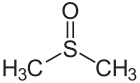 Dimethyl sulfoxide Sulfur-oxygen double bond
 Diazene Nitrogen-nitrogen double bond


 2 sp2 orbitals (total of 3 such orbitals) approach to form a sp2-sp2 sigma bond
 Two p-orbitals overlap to form a pi-bond in a plane parallel to the sigma plane