Network science

From Wikipedia, the free encyclopedia

https://en.wikipedia.org/wiki/Network_science

Network science is an academic field which studies complex networks such as telecommunication networks, computer networks, biological networks, cognitive and semantic networks, and social networks, considering distinct elements or actors represented by nodes (or vertices) and the connections between the elements or actors as links (or edges). The field draws on theories and methods including graph theory from mathematics, statistical mechanics from physics, data mining and information visualization from computer science, inferential modeling from statistics, and social structure from sociology. The United States National Research Council defines network science as "the study of network representations of physical, biological, and social phenomena leading to predictive models of these phenomena."

Background and history

The study of networks has emerged in diverse disciplines as a means of analyzing complex relational data. The earliest known paper in this field is the famous Seven Bridges of Königsberg written by Leonhard Euler in 1736. Euler's mathematical description of vertices and edges was the foundation of graph theory, a branch of mathematics that studies the properties of pairwise relations in a network structure. The field of graph theory continued to develop and found applications in chemistry (Sylvester, 1878).

Dénes Kőnig, a Hungarian mathematician and professor, wrote the first book in Graph Theory, entitled "Theory of finite and infinite graphs", in 1936.

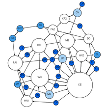
Moreno's sociogram of a 1st grade class.

In the 1930s Jacob Moreno, a psychologist in the Gestalt tradition, arrived in the United States. He developed the sociogram and presented it to the public in April 1933 at a convention of medical scholars. Moreno claimed that "before the advent of sociometry no one knew what the interpersonal structure of a group 'precisely' looked like" (Moreno, 1953). The sociogram was a representation of the social structure of a group of elementary school students. The boys were friends of boys and the girls were friends of girls with the exception of one boy who said he liked a single girl. The feeling was not reciprocated. This network representation of social structure was found so intriguing that it was printed in The New York Times (April 3, 1933, page 17). The sociogram has found many applications and has grown into the field of social network analysis.

Probabilistic theory in network science developed as an offshoot of graph theory with Paul Erdős and Alfréd Rényi's eight famous papers on random graphs. For social networks the exponential random graph model or p* is a notational framework used to represent the probability space of a tie occurring in a social network. An alternate approach to network probability structures is the network probability matrix, which models the probability of edges occurring in a network, based on the historic presence or absence of the edge in a sample of networks.

In 1998, David Krackhardt and Kathleen Carley introduced the idea of a meta-network with the PCANS Model. They suggest that "all organizations are structured along these three domains, Individuals, Tasks, and Resources". Their paper introduced the concept that networks occur across multiple domains and that they are interrelated. This field has grown into another sub-discipline of network science called dynamic network analysis.

More recently other network science efforts have focused on mathematically describing different network topologies. Duncan Watts and Steven Strogatz reconciled empirical data on networks with mathematical representation, describing the small-world network. Albert-László Barabási and Reka Albert discovered scale-free networks, a property that captures the fact that in real network hubs coexist with many small degree vertices, and offered a dynamical model to explain the origin of this scale-free state.

Department of Defense initiatives

The U.S. military first became interested in network-centric warfare as an operational concept based on network science in 1996. John A. Parmentola, the U.S. Army Director for Research and Laboratory Management, proposed to the Army's Board on Science and Technology (BAST) on December 1, 2003 that Network Science become a new Army research area. The BAST, the Division on Engineering and Physical Sciences for the National Research Council (NRC) of the National Academies, serves as a convening authority for the discussion of science and technology issues of importance to the Army and oversees independent Army-related studies conducted by the National Academies. The BAST conducted a study to find out whether identifying and funding a new field of investigation in basic research, Network Science, could help close the gap between what is needed to realize Network-Centric Operations and the current primitive state of fundamental knowledge of networks.

As a result, the BAST issued the NRC study in 2005 titled Network Science (referenced above) that defined a new field of basic research in Network Science for the Army. Based on the findings and recommendations of that study and the subsequent 2007 NRC report titled Strategy for an Army Center for Network Science, Technology, and Experimentation, Army basic research resources were redirected to initiate a new basic research program in Network Science. To build a new theoretical foundation for complex networks, some of the key Network Science research efforts now ongoing in Army laboratories address:

• Mathematical models of network behavior to predict performance with network size, complexity, and environment
• Optimized human performance required for network-enabled warfare
• Networking within ecosystems and at the molecular level in cells.

As initiated in 2004 by Frederick I. Moxley with support he solicited from David S. Alberts, the Department of Defense helped to establish the first Network Science Center in conjunction with the U.S. Army at the United States Military Academy (USMA). Under the tutelage of Dr. Moxley and the faculty of the USMA, the first interdisciplinary undergraduate courses in Network Science were taught to cadets at West Point. In order to better instill the tenets of network science among its cadre of future leaders, the USMA has also instituted a five-course undergraduate minor in Network Science. 

In 2006, the U.S. Army and the United Kingdom (UK) formed the Network and Information Science International Technology Alliance, a collaborative partnership among the Army Research Laboratory, UK Ministry of Defense and a consortium of industries and universities in the U.S. and UK. The goal of the alliance is to perform basic research in support of Network- Centric Operations across the needs of both nations.

In 2009, the U.S. Army formed the Network Science CTA, a collaborative research alliance among the Army Research Laboratory, CERDEC, and a consortium of about 30 industrial R&D labs and universities in the U.S. The goal of the alliance is to develop a deep understanding of the underlying commonalities among intertwined social/cognitive, information, and communications networks, and as a result improve our ability to analyze, predict, design, and influence complex systems interweaving many kinds of networks.

Subsequently, as a result of these efforts, the U.S. Department of Defense has sponsored numerous research projects that support Network Science.

Network Classification

Deterministic Network

The definition of deterministic network is defined compared with the definition of probabilistic network. In un-weighted deterministic networks, edges either exist or not, usually we use 0 to represent non-existence of an edge while 1 to represent existence of an edge. In weighted deterministic networks, the edge value represents the weight of each edge, for example, the strength level.

Probabilistic Network

In probabilistic networks, values behind each edge represent the likelihood of the existence of each edge. For example, if one edge has a value equals to 0.9, we say the existence probability of this edge is 0.9.

Network properties

Often, networks have certain attributes that can be calculated to analyze the properties & characteristics of the network. The behavior of these network properties often define network models and can be used to analyze how certain models contrast to each other. Many of the definitions for other terms used in network science can be found in Glossary of graph theory.

Size

The size of a network can refer to the number of nodes ${\displaystyle N}$ or, less commonly, the number of edges ${\displaystyle E}$ which (for connected graphs with no multi-edges) can range from ${\displaystyle N-1}$ (a tree) to ${\displaystyle E_{max}}$ (a complete graph). In the case of a simple graph (a network in which at most one (undirected) edge exists between each pair of vertices, and in which no vertices connect to themselves), we have ${\displaystyle E_{max}=(\genfrac{}{}{0ex}{}{N}{2})=N(N-1)/2}$; for directed graphs (with no self-connected nodes), ${\displaystyle E_{max}=N(N-1)}$; for directed graphs with self-connections allowed, ${\displaystyle E_{max}=N^2}$. In the circumstance of a graph within which multiple edges may exist between a pair of vertices, ${\displaystyle E_{max}=\mathrm{\infty }}$.

Density

The density ${\displaystyle D}$ of a network is defined as a normalized ratio between 0 and 1 of the number of edges ${\displaystyle E}$ to the number of possible edges in a network with ${\displaystyle N}$ nodes. Network density is a measure of the percentage of "optional" edges that exist in the network and can be computed as ${\displaystyle D=\frac{E-E_{\mathrm{m}\mathrm{i}\mathrm{n}}}{E_{\mathrm{m}\mathrm{a}\mathrm{x}}-E_{\mathrm{m}\mathrm{i}\mathrm{n}}}}$ where ${\displaystyle E_{\mathrm{m}\mathrm{i}\mathrm{n}}}$ and ${\displaystyle E_{\mathrm{m}\mathrm{a}\mathrm{x}}}$ are the minimum and maximum number of edges in a connected network with ${\displaystyle N}$ nodes, respectively. In the case of simple graphs, ${\displaystyle E_{\mathrm{m}\mathrm{a}\mathrm{x}}}$ is given by the binomial coefficient ${\displaystyle (\genfrac{}{}{0ex}{}{N}{2})}$ and ${\displaystyle E_{\mathrm{m}\mathrm{i}\mathrm{n}}=N-1}$, giving density ${\displaystyle D=\frac{E-(N-1)}{E_{\mathrm{m}\mathrm{a}\mathrm{x}}-(N-1)}=\frac{2(E-N+1)}{N(N-3)+2}}$. Another possible equation is ${\displaystyle D=\frac{T-2N+2}{N(N-3)+2},}$ whereas the ties ${\displaystyle T}$ are unidirectional (Wasserman & Faust 1994). This gives a better overview over the network density, because unidirectional relationships can be measured.

Planar network density

The density ${\displaystyle D}$ of a network, where there is no intersection between edges, is defined as a ratio of the number of edges ${\displaystyle E}$ to the number of possible edges in a network with ${\displaystyle N}$ nodes, given by a graph with no intersecting edges ${\displaystyle (E_{max}=3N-6)}$, giving ${\displaystyle D=\frac{E-N+1}{2N-5}.}$

Average degree

The degree ${\displaystyle k}$ of a node is the number of edges connected to it. Closely related to the density of a network is the average degree, ${\displaystyle ⟨k⟩=\frac{2E}{N}}$ (or, in the case of directed graphs, ${\displaystyle ⟨k⟩=\frac{E}{N}}$, the former factor of 2 arising from each edge in an undirected graph contributing to the degree of two distinct vertices). In the ER random graph model (${\displaystyle G(N,p)}$) we can compute the expected value of ${\displaystyle ⟨k⟩}$ (equal to the expected value of ${\displaystyle k}$ of an arbitrary vertex): a random vertex has ${\displaystyle N-1}$ other vertices in the network available, and with probability ${\displaystyle p}$, connects to each. Thus, ${\displaystyle \mathbb{E}[⟨k⟩]=\mathbb{E}[k]=p(N-1)}$.

Average shortest path length (or characteristic path length)

The average shortest path length is calculated by finding the shortest path between all pairs of nodes, and taking the average over all paths of the length thereof (the length being the number of intermediate edges contained in the path, i.e., the distance ${\displaystyle d_{u,v}}$ between the two vertices ${\displaystyle u,v}$ within the graph). This shows us, on average, the number of steps it takes to get from one member of the network to another. The behavior of the expected average shortest path length (that is, the ensemble average of the average shortest path length) as a function of the number of vertices ${\displaystyle N}$ of a random network model defines whether that model exhibits the small-world effect; if it scales as ${\displaystyle O(\ln N)}$, the model generates small-world nets. For faster-than-logarithmic growth, the model does not produce small worlds. The special case of ${\displaystyle O(\ln \ln N)}$ is known as ultra-small world effect.

Diameter of a network

As another means of measuring network graphs, we can define the diameter of a network as the longest of all the calculated shortest paths in a network. It is the shortest distance between the two most distant nodes in the network. In other words, once the shortest path length from every node to all other nodes is calculated, the diameter is the longest of all the calculated path lengths. The diameter is representative of the linear size of a network. If node A-B-C-D are connected, going from A->D this would be the diameter of 3 (3-hops, 3-links).

Clustering coefficient

The clustering coefficient is a measure of an "all-my-friends-know-each-other" property. This is sometimes described as the friends of my friends are my friends. More precisely, the clustering coefficient of a node is the ratio of existing links connecting a node's neighbors to each other to the maximum possible number of such links. The clustering coefficient for the entire network is the average of the clustering coefficients of all the nodes. A high clustering coefficient for a network is another indication of a small world.

The clustering coefficient of the ${\displaystyle i}$'th node is

${\displaystyle C_i=\frac{2e_i}{k_i(k_i-1)},}$

where ${\displaystyle k_i}$ is the number of neighbours of the ${\displaystyle i}$'th node, and ${\displaystyle e_i}$ is the number of connections between these neighbours. The maximum possible number of connections between neighbors is, then,

${\displaystyle (\genfrac{}{}{0ex}{}{k}{2})=\frac{k(k-1)}{2}.}$

From a probabilistic standpoint, the expected local clustering coefficient is the likelihood of a link existing between two arbitrary neighbors of the same node.

Connectedness

The way in which a network is connected plays a large part into how networks are analyzed and interpreted. Networks are classified in four different categories:

• Clique/Complete Graph: a completely connected network, where all nodes are connected to every other node. These networks are symmetric in that all nodes have in-links and out-links from all others.
• Giant Component: A single connected component which contains most of the nodes in the network.
• Weakly Connected Component: A collection of nodes in which there exists a path from any node to any other, ignoring directionality of the edges.
• Strongly Connected Component: A collection of nodes in which there exists a directed path from any node to any other.

Node centrality

Main article: Centrality

Centrality indices produce rankings which seek to identify the most important nodes in a network model. Different centrality indices encode different contexts for the word "importance." The betweenness centrality, for example, considers a node highly important if it form bridges between many other nodes. The eigenvalue centrality, in contrast, considers a node highly important if many other highly important nodes link to it. Hundreds of such measures have been proposed in the literature.

Centrality indices are only accurate for identifying the most important nodes. The measures are seldom, if ever, meaningful for the remainder of network nodes. Also, their indications are only accurate within their assumed context for importance, and tend to "get it wrong" for other contexts. For example, imagine two separate communities whose only link is an edge between the most junior member of each community. Since any transfer from one community to the other must go over this link, the two junior members will have high betweenness centrality. But, since they are junior, (presumably) they have few connections to the "important" nodes in their community, meaning their eigenvalue centrality would be quite low.

Node influence

Main article: Node influence metric

Limitations to centrality measures have led to the development of more general measures. Two examples are the accessibility, which uses the diversity of random walks to measure how accessible the rest of the network is from a given start node, and the expected force, derived from the expected value of the force of infection generated by a node. Both of these measures can be meaningfully computed from the structure of the network alone.

Community structure

Main article: Community structure

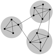
Fig. 1: A sketch of a small network displaying community structure, with three groups of nodes with dense internal connections and sparser connections between groups.

Nodes in a network may be partitioned into groups representing communities. Depending on the context, communities may be distinct or overlapping. Typically, nodes in such communities will be strongly connected to other nodes in the same community, but weakly connected to nodes outside the community. In the absence of a ground truth describing the community structure of a specific network, several algorithms have been developed to infer possible community structures using either supervised of unsupervised clustering methods.

Network models

Network models serve as a foundation to understanding interactions within empirical complex networks. Various random graph generation models produce network structures that may be used in comparison to real-world complex networks.

Erdős–Rényi random graph model

This Erdős–Rényi model is generated with N = 4 nodes. For each edge in the complete graph formed by all N nodes, a random number is generated and compared to a given probability. If the random number is less than p, an edge is formed on the model.

The Erdős–Rényi model, named for Paul Erdős and Alfréd Rényi, is used for generating random graphs in which edges are set between nodes with equal probabilities. It can be used in the probabilistic method to prove the existence of graphs satisfying various properties, or to provide a rigorous definition of what it means for a property to hold for almost all graphs.

To generate an Erdős–Rényi model ${\displaystyle G(n,p)}$ two parameters must be specified: the total number of nodes n and the probability p that a random pair of nodes has an edge.

Because the model is generated without bias to particular nodes, the degree distribution is binomial: for a randomly chosen vertex ${\displaystyle v}$,

${\displaystyle P(\mathrm{deg}(v)=k)=(\genfrac{}{}{0ex}{}{n-1}{k})p^k(1-p{)}^{n-1-k}.}$

In this model the clustering coefficient is 0 a.s. The behavior of ${\displaystyle G(n,p)}$ can be broken into three regions.

Subcritical ${\displaystyle np<1}$: All components are simple and very small, the largest component has size ${\displaystyle |C_1|=O(\log n)}$;

Critical ${\displaystyle np=1}$: ${\displaystyle |C_1|=O(n^{\frac{2}{3}})}$;

Supercritical ${\displaystyle np>1}$:${\displaystyle |C_1|\approx yn}$ where ${\displaystyle y=y(np)}$ is the positive solution to the equation ${\displaystyle e^{-pny}=1-y}$.

The largest connected component has high complexity. All other components are simple and small ${\displaystyle |C_2|=O(\log n)}$.

Configuration model

The configuration model takes a degree sequence or degree distribution (which subsequently is used to generate a degree sequence) as the input, and produces randomly connected graphs in all respects other than the degree sequence. This means that for a given choice of the degree sequence, the graph is chosen uniformly at random from the set of all graphs that comply with this degree sequence. The degree ${\displaystyle k}$ of a randomly chosen vertex is an independent and identically distributed random variable with integer values. When $\mathbb{E}[k^2]-2\mathbb{E}[k]>0$, the configuration graph contains the giant connected component, which has infinite size. The rest of the components have finite sizes, which can be quantified with the notion of the size distribution. The probability ${\displaystyle w(n)}$ that a randomly sampled node is connected to a component of size ${\displaystyle n}$ is given by convolution powers of the degree distribution:

$${\displaystyle w(n)=\{\begin{array}{ll}\frac{\mathbb{E}[k]}{n-1}{u}_1^{\ast n}(n-2),& n>1,\\ u(0)& n=1,\end{array}}$$

where ${\displaystyle u(k)}$ denotes the degree distribution and ${\displaystyle u_1(k)=\frac{(k+1)u(k+1)}{\mathbb{E}[k]}}$. The giant component can be destroyed by randomly removing the critical fraction ${\displaystyle p_c}$ of all edges. This process is called percolation on random networks. When the second moment of the degree distribution is finite, $\mathbb{E}[k^2]<\mathrm{\infty }$, this critical edge fraction is given by ${\displaystyle p_c=1-\frac{\mathbb{E}[k]}{\mathbb{E}[k^2]-\mathbb{E}[k]}}$, and the average vertex-vertex distance ${\displaystyle l}$ in the giant component scales logarithmically with the total size of the network, ${\displaystyle l=O(\log N)}$.

In the directed configuration model, the degree of a node is given by two numbers, in-degree ${\displaystyle k_{\text{in}}}$ and out-degree ${\displaystyle k_{\text{out}}}$, and consequently, the degree distribution is two-variate. The expected number of in-edges and out-edges coincides, so that $\mathbb{E}[k_{\text{in}}]=\mathbb{E}[k_{\text{out}}]$. The directed configuration model contains the giant component iff

$${\displaystyle 2\mathbb{E}[k_{\text{in}}]\mathbb{E}[k_{\text{in}}{k}_{\text{out}}]-\mathbb{E}[k_{\text{in}}]\mathbb{E}[k_{\text{out}}^2]-\mathbb{E}[k_{\text{in}}]\mathbb{E}[k_{\text{in}}^2]+\mathbb{E}[k_{\text{in}}^2]\mathbb{E}[k_{\text{out}}^2]-\mathbb{E}[k_{\text{in}}{k}_{\text{out}}{]}^2>0.}$$

Note that $\mathbb{E}[k_{\text{in}}]$ and $\mathbb{E}[k_{\text{out}}]$ are equal and therefore interchangeable in the latter inequality. The probability that a randomly chosen vertex belongs to a component of size ${\displaystyle n}$ is given by:

$${\displaystyle h_{\text{in}}(n)=\frac{\mathbb{E}[k_{in}]}{n-1}{\tilde{u}}_{\text{in}}^{\ast n}(n-2),n>1,{\tilde{u}}_{\text{in}}=\frac{k_{\text{in}}+1}{\mathbb{E}[k_{\text{in}}]}\sum _{k_{\text{out}}\ge 0}u(k_{\text{in}}+1,k_{\text{out}}),}$$

for in-components, and

${\displaystyle h_{\text{out}}(n)=\frac{\mathbb{E}[k_{\text{out}}]}{n-1}{\tilde{u}}_{\text{out}}^{\ast n}(n-2),n>1,{\tilde{u}}_{\text{out}}=\frac{k_{\text{out}}+1}{\mathbb{E}[k_{\text{out}}]}\sum _{k_{\text{in}}\ge 0}u(k_{\text{in}},k_{\text{out}}+1),}$

for out-components.

Watts–Strogatz small world model

The Watts and Strogatz model uses the concept of rewiring to achieve its structure. The model generator will iterate through each edge in the original lattice structure. An edge may change its connected vertices according to a given rewiring probability. ${\displaystyle ⟨k⟩=4}$ in this example.

The Watts and Strogatz model is a random graph generation model that produces graphs with small-world properties.

An initial lattice structure is used to generate a Watts–Strogatz model. Each node in the network is initially linked to its ${\displaystyle ⟨k⟩}$ closest neighbors. Another parameter is specified as the rewiring probability. Each edge has a probability ${\displaystyle p}$ that it will be rewired to the graph as a random edge. The expected number of rewired links in the model is ${\displaystyle pE=pN⟨k⟩/2}$.

As the Watts–Strogatz model begins as non-random lattice structure, it has a very high clustering coefficient along with high average path length. Each rewire is likely to create a shortcut between highly connected clusters. As the rewiring probability increases, the clustering coefficient decreases slower than the average path length. In effect, this allows the average path length of the network to decrease significantly with only slightly decreases in clustering coefficient. Higher values of p force more rewired edges, which in effect makes the Watts–Strogatz model a random network.

Barabási–Albert (BA) preferential attachment model

The Barabási–Albert model is a random network model used to demonstrate a preferential attachment or a "rich-get-richer" effect. In this model, an edge is most likely to attach to nodes with higher degrees. The network begins with an initial network of m₀ nodes. m₀ ≥ 2 and the degree of each node in the initial network should be at least 1, otherwise it will always remain disconnected from the rest of the network.

In the BA model, new nodes are added to the network one at a time. Each new node is connected to ${\displaystyle m}$ existing nodes with a probability that is proportional to the number of links that the existing nodes already have. Formally, the probability p_i that the new node is connected to node i is

${\displaystyle p_i=\frac{k_i}{\sum _j{k}_j},}$

where k_i is the degree of node i. Heavily linked nodes ("hubs") tend to quickly accumulate even more links, while nodes with only a few links are unlikely to be chosen as the destination for a new link. The new nodes have a "preference" to attach themselves to the already heavily linked nodes.

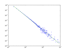
The degree distribution of the BA Model, which follows a power law. In loglog scale the power law function is a straight line.

The degree distribution resulting from the BA model is scale free, in particular, for large degree it is a power law of the form:

${\displaystyle P(k)\sim k^{-3}}$

Hubs exhibit high betweenness centrality which allows short paths to exist between nodes. As a result, the BA model tends to have very short average path lengths. The clustering coefficient of this model also tends to 0.

The Barabási–Albert model was developed for undirected networks, aiming to explain the universality of the scale-free property, and applied to a wide range of different networks and applications. The directed version of this model is the Price model which was developed to just citation networks.

Non-linear preferential attachment

Main article: Non-linear preferential attachment

In non-linear preferential attachment (NLPA), existing nodes in the network gain new edges proportionally to the node degree raised to a constant positive power, ${\displaystyle \alpha }$. Formally, this means that the probability that node ${\displaystyle i}$ gains a new edge is given by

${\displaystyle p_i=\frac{k_i^{\alpha }}{\sum _j{k}_j^{\alpha }}.}$

If ${\displaystyle \alpha =1}$, NLPA reduces to the BA model and is referred to as "linear". If ${\displaystyle 0<\alpha <1}$, NLPA is referred to as "sub-linear" and the degree distribution of the network tends to a stretched exponential distribution. If ${\displaystyle \alpha >1}$, NLPA is referred to as "super-linear" and a small number of nodes connect to almost all other nodes in the network. For both ${\displaystyle \alpha <1}$ and ${\displaystyle \alpha >1}$, the scale-free property of the network is broken in the limit of infinite system size. However, if ${\displaystyle \alpha }$ is only slightly larger than ${\displaystyle 1}$, NLPA may result in degree distributions which appear to be transiently scale free.

Mediation-driven attachment (MDA) model

In the mediation-driven attachment (MDA) model in which a new node coming with ${\displaystyle m}$ edges picks an existing connected node at random and then connects itself not with that one but with ${\displaystyle m}$ of its neighbors chosen also at random. The probability ${\displaystyle \mathrm{\Pi }(i)}$ that the node ${\displaystyle i}$ of the existing node picked is

${\displaystyle \mathrm{\Pi }(i)=\frac{k_i}{N}\frac{\sum _{j=1}^{k_i}\frac{1}{k_j}}{k_i}.}$

The factor ${\displaystyle \frac{\sum _{j=1}^{k_i}\frac{1}{k_j}}{k_i}}$ is the inverse of the harmonic mean (IHM) of degrees of the ${\displaystyle k_i}$ neighbors of a node ${\displaystyle i}$. Extensive numerical investigation suggest that for an approximately ${\displaystyle m>14}$ the mean IHM value in the large ${\displaystyle N}$ limit becomes a constant which means ${\displaystyle \mathrm{\Pi }(i)\propto k_i}$. It implies that the higher the links (degree) a node has, the higher its chance of gaining more links since they can be reached in a larger number of ways through mediators which essentially embodies the intuitive idea of rich get richer mechanism (or the preferential attachment rule of the Barabasi–Albert model). Therefore, the MDA network can be seen to follow the PA rule but in disguise.

However, for ${\displaystyle m=1}$ it describes the winner takes it all mechanism as we find that almost ${\displaystyle 99\mathrm{\%}}$ of the total nodes have degree one and one is super-rich in degree. As ${\displaystyle m}$ value increases the disparity between the super rich and poor decreases and as ${\displaystyle m>14}$ we find a transition from rich get super richer to rich get richer mechanism.

Fitness model

Another model where the key ingredient is the nature of the vertex has been introduced by Caldarelli et al. Here a link is created between two vertices ${\displaystyle i,j}$ with a probability given by a linking function ${\displaystyle f({\eta }_i,{\eta }_j)}$ of the fitnesses of the vertices involved. The degree of a vertex i is given by 

${\displaystyle k({\eta }_i)=N{\int }_0^{\mathrm{\infty }}f({\eta }_i,{\eta }_j)\rho ({\eta }_j)d{\eta }_j}$

If ${\displaystyle k({\eta }_i)}$ is an invertible and increasing function of ${\displaystyle {\eta }_i}$, then the probability distribution ${\displaystyle P(k)}$ is given by

${\displaystyle P(k)=\rho (\eta (k))\cdot {\eta }^{\prime }(k)}$

As a result, if the fitnesses ${\displaystyle \eta }$ are distributed as a power law, then also the node degree does.

Less intuitively with a fast decaying probability distribution as ${\displaystyle \rho (\eta )=e^{-\eta }}$ together with a linking function of the kind

${\displaystyle f({\eta }_i,{\eta }_j)=\mathrm{\Theta }({\eta }_i+{\eta }_j-Z)}$

with ${\displaystyle Z}$ a constant and ${\displaystyle \mathrm{\Theta }}$ the Heavyside function, we also obtain scale-free networks.

Such model has been successfully applied to describe trade between nations by using GDP as fitness for the various nodes ${\displaystyle i,j}$ and a linking function of the kind 

${\displaystyle \frac{\delta {\eta }_i{\eta }_j}{1+\delta {\eta }_i{\eta }_j}.}$

Exponential random graph models

Exponential Random Graph Models (ERGMs) are a family of statistical models for analyzing data from social and other networks. The Exponential family is a broad family of models for covering many types of data, not just networks. An ERGM is a model from this family which describes networks.

We adopt the notation to represent a random graph ${\displaystyle Y\in \mathcal{Y}}$ via a set of ${\displaystyle n}$ nodes and a collection of tie variables ${\displaystyle \{Y_{ij}:i=1,\dots ,n;j=1,\dots ,n\}}$, indexed by pairs of nodes ${\displaystyle ij}$, where ${\displaystyle Y_{ij}=1}$ if the nodes ${\displaystyle (i,j)}$ are connected by an edge and ${\displaystyle Y_{ij}=0}$ otherwise.

The basic assumption of ERGMs is that the structure in an observed graph ${\displaystyle y}$ can be explained by a given vector of sufficient statistics ${\displaystyle s(y)}$ which are a function of the observed network and, in some cases, nodal attributes. The probability of a graph ${\displaystyle y\in \mathcal{Y}}$ in an ERGM is defined by:

${\displaystyle P(Y=y|\theta )=\frac{\exp ({\theta }^{T}s(y))}{c(\theta )}}$

where ${\displaystyle \theta }$ is a vector of model parameters associated with ${\displaystyle s(y)}$ and ${\displaystyle c(\theta )=\sum _{y^{\prime }\in \mathcal{Y}}\exp ({\theta }^{T}s(y^{\prime }))}$ is a normalising constant.

Network analysis

Social network analysis

Social network analysis examines the structure of relationships between social entities. These entities are often persons, but may also be groups, organizations, nation states, web sites, scholarly publications.

Since the 1970s, the empirical study of networks has played a central role in social science, and many of the mathematical and statistical tools used for studying networks have been first developed in sociology. Amongst many other applications, social network analysis has been used to understand the diffusion of innovations, news and rumors. Similarly, it has been used to examine the spread of both diseases and health-related behaviors. It has also been applied to the study of markets, where it has been used to examine the role of trust in exchange relationships and of social mechanisms in setting prices. Similarly, it has been used to study recruitment into political movements and social organizations. It has also been used to conceptualize scientific disagreements as well as academic prestige. In the second language acquisition literature, it has an established history in study abroad research, revealing how peer learner interaction networks influence their language progress. More recently, network analysis (and its close cousin traffic analysis) has gained a significant use in military intelligence, for uncovering insurgent networks of both hierarchical and leaderless nature. In criminology, it is being used to identify influential actors in criminal gangs, offender movements, co-offending, predict criminal activities and make policies.

Dynamic network analysis

Dynamic network analysis examines the shifting structure of relationships among different classes of entities in complex socio-technical systems effects, and reflects social stability and changes such as the emergence of new groups, topics, and leaders. Dynamic Network Analysis focuses on meta-networks composed of multiple types of nodes (entities) and multiple types of links. These entities can be highly varied. Examples include people, organizations, topics, resources, tasks, events, locations, and beliefs.

Dynamic network techniques are particularly useful for assessing trends and changes in networks over time, identification of emergent leaders, and examining the co-evolution of people and ideas.

Biological network analysis

With the recent explosion of publicly available high throughput biological data, the analysis of molecular networks has gained significant interest. The type of analysis in this content are closely related to social network analysis, but often focusing on local patterns in the network. For example, network motifs are small subgraphs that are over-represented in the network. Activity motifs are similar over-represented patterns in the attributes of nodes and edges in the network that are over represented given the network structure. The analysis of biological networks has led to the development of network medicine, which looks at the effect of diseases in the interactome.

Link analysis

Link analysis is a subset of network analysis, exploring associations between objects. An example may be examining the addresses of suspects and victims, the telephone numbers they have dialed and financial transactions that they have partaken in during a given timeframe, and the familial relationships between these subjects as a part of police investigation. Link analysis here provides the crucial relationships and associations between very many objects of different types that are not apparent from isolated pieces of information. Computer-assisted or fully automatic computer-based link analysis is increasingly employed by banks and insurance agencies in fraud detection, by telecommunication operators in telecommunication network analysis, by medical sector in epidemiology and pharmacology, in law enforcement investigations, by search engines for relevance rating (and conversely by the spammers for spamdexing and by business owners for search engine optimization), and everywhere else where relationships between many objects have to be analyzed.

Pandemic analysis

The SIR model is one of the most well known algorithms on predicting the spread of global pandemics within an infectious population.

Susceptible to infected

${\displaystyle S=\beta \left(\frac{1}{N}\right)}$

The formula above describes the "force" of infection for each susceptible unit in an infectious population, where β is equivalent to the transmission rate of said disease.

To track the change of those susceptible in an infectious population:

${\displaystyle \mathrm{\Delta }S=\beta \times S\frac{1}{N}\mathrm{\Delta }t}$

Infected to recovered

${\displaystyle \mathrm{\Delta }I=\mu I\mathrm{\Delta }t}$

Over time, the number of those infected fluctuates by: the specified rate of recovery, represented by ${\displaystyle \mu }$ but deducted to one over the average infectious period ${\displaystyle \frac{1}{\tau }}$, the numbered of infectious individuals, ${\displaystyle I}$, and the change in time, ${\displaystyle \mathrm{\Delta }t}$.

Infectious period

Whether a population will be overcome by a pandemic, with regards to the SIR model, is dependent on the value of ${\displaystyle R_0}$ or the "average people infected by an infected individual."

${\displaystyle R_0=\beta \tau =\frac{\beta }{\mu }}$

Web link analysis

Several Web search ranking algorithms use link-based centrality metrics, including (in order of appearance) Marchiori's Hyper Search, Google's PageRank, Kleinberg's HITS algorithm, the CheiRank and TrustRank algorithms. Link analysis is also conducted in information science and communication science in order to understand and extract information from the structure of collections of web pages. For example, the analysis might be of the interlinking between politicians' web sites or blogs.

PageRank

PageRank works by randomly picking "nodes" or websites and then with a certain probability, "randomly jumping" to other nodes. By randomly jumping to these other nodes, it helps PageRank completely traverse the network as some webpages exist on the periphery and would not as readily be assessed.

Each node, ${\displaystyle x_i}$, has a PageRank as defined by the sum of pages ${\displaystyle j}$ that link to ${\displaystyle i}$ times one over the outlinks or "out-degree" of ${\displaystyle j}$ times the "importance" or PageRank of ${\displaystyle j}$.

${\displaystyle x_i=\sum _{j\to i}\frac{1}{N_j}{x}_j^{(k)}}$

Random jumping

As explained above, PageRank enlists random jumps in attempts to assign PageRank to every website on the internet. These random jumps find websites that might not be found during the normal search methodologies such as breadth-first search and depth-first search.

In an improvement over the aforementioned formula for determining PageRank includes adding these random jump components. Without the random jumps, some pages would receive a PageRank of 0 which would not be good.

The first is ${\displaystyle \alpha }$, or the probability that a random jump will occur. Contrasting is the "damping factor", or ${\displaystyle 1-\alpha }$.

${\displaystyle R(p)=\frac{\alpha }{N}+(1-\alpha )\sum _{j\to i}\frac{1}{N_j}{x}_j^{(k)}}$

Another way of looking at it:

${\displaystyle R(A)=\sum \frac{R_B}{B_{\text{(outlinks)}}}+\cdots +\frac{R_n}{n_{\text{(outlinks)}}}}$

Centrality measures

Information about the relative importance of nodes and edges in a graph can be obtained through centrality measures, widely used in disciplines like sociology. Centrality measures are essential when a network analysis has to answer questions such as: "Which nodes in the network should be targeted to ensure that a message or information spreads to all or most nodes in the network?" or conversely, "Which nodes should be targeted to curtail the spread of a disease?". Formally established measures of centrality are degree centrality, closeness centrality, betweenness centrality, eigenvector centrality, and katz centrality. The objective of network analysis generally determines the type of centrality measure(s) to be used.

• Degree centrality of a node in a network is the number of links (vertices) incident on the node.
• Closeness centrality determines how "close" a node is to other nodes in a network by measuring the sum of the shortest distances (geodesic paths) between that node and all other nodes in the network.
• Betweenness centrality determines the relative importance of a node by measuring the amount of traffic flowing through that node to other nodes in the network. This is done by measuring the fraction of paths connecting all pairs of nodes and containing the node of interest. Group Betweenness centrality measures the amount of traffic flowing through a group of nodes.
• Eigenvector centrality is a more sophisticated version of degree centrality where the centrality of a node not only depends on the number of links incident on the node but also the quality of those links. This quality factor is determined by the eigenvectors of the adjacency matrix of the network.
• Katz centrality of a node is measured by summing the geodesic paths between that node and all (reachable) nodes in the network. These paths are weighted, paths connecting the node with its immediate neighbors carry higher weights than those which connect with nodes farther away from the immediate neighbors.

Spread of content in networks

Content in a complex network can spread via two major methods: conserved spread and non-conserved spread. In conserved spread, the total amount of content that enters a complex network remains constant as it passes through. The model of conserved spread can best be represented by a pitcher containing a fixed amount of water being poured into a series of funnels connected by tubes. Here, the pitcher represents the original source and the water is the content being spread. The funnels and connecting tubing represent the nodes and the connections between nodes, respectively. As the water passes from one funnel into another, the water disappears instantly from the funnel that was previously exposed to the water. In non-conserved spread, the amount of content changes as it enters and passes through a complex network. The model of non-conserved spread can best be represented by a continuously running faucet running through a series of funnels connected by tubes. Here, the amount of water from the original source is infinite. Also, any funnels that have been exposed to the water continue to experience the water even as it passes into successive funnels. The non-conserved model is the most suitable for explaining the transmission of most infectious diseases.

The SIR model

In 1927, W. O. Kermack and A. G. McKendrick created a model in which they considered a fixed population with only three compartments, susceptible: ${\displaystyle S(t)}$, infected, ${\displaystyle I(t)}$, and recovered, ${\displaystyle R(t)}$. The compartments used for this model consist of three classes:

• ${\displaystyle S(t)}$ is used to represent the number of individuals not yet infected with the disease at time t, or those susceptible to the disease
• ${\displaystyle I(t)}$ denotes the number of individuals who have been infected with the disease and are capable of spreading the disease to those in the susceptible category
• ${\displaystyle R(t)}$ is the compartment used for those individuals who have been infected and then recovered from the disease. Those in this category are not able to be infected again or to transmit the infection to others.

The flow of this model may be considered as follows:

${\displaystyle \mathcal{S}\to \mathcal{I}\to \mathcal{R}}$

Using a fixed population, ${\displaystyle N=S(t)+I(t)+R(t)}$, Kermack and McKendrick derived the following equations:

${\displaystyle \begin{array}{rl}\frac{dS}{dt}& =-\beta SI\\ \frac{dI}{dt}& =\beta SI-\gamma I\\ \frac{dR}{dt}& =\gamma I\end{array}}$

Several assumptions were made in the formulation of these equations: First, an individual in the population must be considered as having an equal probability as every other individual of contracting the disease with a rate of ${\displaystyle \beta }$, which is considered the contact or infection rate of the disease. Therefore, an infected individual makes contact and is able to transmit the disease with ${\displaystyle \beta N}$ others per unit time and the fraction of contacts by an infected with a susceptible is ${\displaystyle S/N}$. The number of new infections in unit time per infective then is ${\displaystyle \beta N(S/N)}$, giving the rate of new infections (or those leaving the susceptible category) as ${\displaystyle \beta N(S/N)I=\beta SI}$ (Brauer & Castillo-Chavez, 2001). For the second and third equations, consider the population leaving the susceptible class as equal to the number entering the infected class. However, infectives are leaving this class per unit time to enter the recovered/removed class at a rate ${\displaystyle \gamma }$ per unit time (where ${\displaystyle \gamma }$ represents the mean recovery rate, or ${\displaystyle 1/\gamma }$ the mean infective period). These processes which occur simultaneously are referred to as the Law of Mass Action, a widely accepted idea that the rate of contact between two groups in a population is proportional to the size of each of the groups concerned (Daley & Gani, 2005). Finally, it is assumed that the rate of infection and recovery is much faster than the time scale of births and deaths and therefore, these factors are ignored in this model.

More can be read on this model on the Epidemic model page.

The master equation approach

A master equation can express the behaviour of an undirected growing network where, at each time step, a new node is added to the network, linked to an old node (randomly chosen and without preference). The initial network is formed by two nodes and two links between them at time ${\displaystyle t=2}$, this configuration is necessary only to simplify further calculations, so at time ${\displaystyle t=n}$ the network have ${\displaystyle n}$ nodes and ${\displaystyle n}$ links.

The master equation for this network is:

${\displaystyle p(k,s,t+1)=\frac{1}{t}p(k-1,s,t)+\left(1-\frac{1}{t}\right)p(k,s,t),}$

where ${\displaystyle p(k,s,t)}$ is the probability to have the node ${\displaystyle s}$ with degree ${\displaystyle k}$ at time ${\displaystyle t+1}$, and ${\displaystyle s}$ is the time step when this node was added to the network. Note that there are only two ways for an old node ${\displaystyle s}$ to have ${\displaystyle k}$ links at time ${\displaystyle t+1}$:

• The node ${\displaystyle s}$ have degree ${\displaystyle k-1}$ at time ${\displaystyle t}$ and will be linked by the new node with probability ${\displaystyle 1/t}$
• Already has degree ${\displaystyle k}$ at time ${\displaystyle t}$ and will not be linked by the new node.

After simplifying this model, the degree distribution is ${\displaystyle P(k)=2^{-k}.}$

Based on this growing network, an epidemic model is developed following a simple rule: Each time the new node is added and after choosing the old node to link, a decision is made: whether or not this new node will be infected. The master equation for this epidemic model is:

${\displaystyle p_r(k,s,t)=r_t\frac{1}{t}{p}_r(k-1,s,t)+\left(1-\frac{1}{t}\right)p_r(k,s,t),}$

where ${\displaystyle r_t}$ represents the decision to infect (${\displaystyle r_t=1}$) or not (${\displaystyle r_t=0}$). Solving this master equation, the following solution is obtained: ${\displaystyle {\tilde{P}}_r(k)={\left(\frac{r}{2}\right)}^k.}$

Multilayer networks

Main article: Multidimensional network

Multilayer networks are networks with multiple kinds of relations. Attempts to model real-world systems as multidimensional networks have been used in various fields such as social network analysis, economics, history, urban and international transport, ecology, psychology, medicine, biology, commerce, climatology, physics, computational neuroscience, operations management, and finance.

Network optimization

Network problems that involve finding an optimal way of doing something are studied under the name of combinatorial optimization. Examples include network flow, shortest path problem, transport problem, transshipment problem, location problem, matching problem, assignment problem, packing problem, routing problem, critical path analysis and PERT (Program Evaluation & Review Technique).

Interdependent networks

Interdependent networks are networks where the functioning of nodes in one network depends on the functioning of nodes in another network. In nature, networks rarely appear in isolation, rather, usually networks are typically elements in larger systems, and interact with elements in that complex system. Such complex dependencies can have non-trivial effects on one another. A well studied example is the interdependency of infrastructure networks, the power stations which form the nodes of the power grid require fuel delivered via a network of roads or pipes and are also controlled via the nodes of communications network. Though the transportation network does not depend on the power network to function, the communications network does. In such infrastructure networks, the disfunction of a critical number of nodes in either the power network or the communication network can lead to cascading failures across the system with potentially catastrophic result to the whole system functioning. If the two networks were treated in isolation, this important feedback effect would not be seen and predictions of network robustness would be greatly overestimated.

Genetic disorder

From Wikipedia, the free encyclopedia

https://en.wikipedia.org/wiki/Genetic_disorder

Genetic disorder
A boy with Down syndrome, one of the most common genetic disorders
Specialty	Medical genetics

Diagram featuring examples of a disease located on each chromosome

A genetic disorder is a health problem caused by one or more abnormalities in the genome. It can be caused by a mutation in a single gene (monogenic) or multiple genes (polygenic) or by a chromosomal abnormality. Although polygenic disorders are the most common, the term is mostly used when discussing disorders with a single genetic cause, either in a gene or chromosome. The mutation responsible can occur spontaneously before embryonic development (a de novo mutation), or it can be inherited from two parents who are carriers of a faulty gene (autosomal recessive inheritance) or from a parent with the disorder (autosomal dominant inheritance). When the genetic disorder is inherited from one or both parents, it is also classified as a hereditary disease. Some disorders are caused by a mutation on the X chromosome and have X-linked inheritance. Very few disorders are inherited on the Y chromosome or mitochondrial DNA (due to their size).

There are well over 6,000 known genetic disorders, and new genetic disorders are constantly being described in medical literature. More than 600 genetic disorders are treatable. Around 1 in 50 people are affected by a known single-gene disorder, while around 1 in 263 are affected by a chromosomal disorder. Around 65% of people have some kind of health problem as a result of congenital genetic mutations. Due to the significantly large number of genetic disorders, approximately 1 in 21 people are affected by a genetic disorder classified as "rare" (usually defined as affecting less than 1 in 2,000 people). Most genetic disorders are rare in themselves.

Genetic disorders are present before birth, and some genetic disorders produce birth defects, but birth defects can also be developmental rather than hereditary. The opposite of a hereditary disease is an acquired disease. Most cancers, although they involve genetic mutations to a small proportion of cells in the body, are acquired diseases. Some cancer syndromes, however, such as BRCA mutations, are hereditary genetic disorders.

Single-gene

Prevalence of some single-gene disorders

Disorder prevalence (approximate)
Autosomal dominant
Familial hypercholesterolemia	1 in 500
Myotonic dystrophy type 1	1 in 2,100
Neurofibromatosis type I	1 in 2,500
Hereditary spherocytosis	1 in 5,000
Marfan syndrome	1 in 4,000
Huntington's disease	1 in 15,000
Autosomal recessive
Sickle cell anaemia	1 in 625
Cystic fibrosis	1 in 2,000
Tay–Sachs disease	1 in 3,000
Phenylketonuria	1 in 12,000
Autosomal recessive polycystic kidney disease	1 in 20,000
Mucopolysaccharidoses	1 in 25,000
Lysosomal acid lipase deficiency	1 in 40,000
Glycogen storage diseases	1 in 50,000
Galactosemia	1 in 57,000
X-linked
Duchenne muscular dystrophy	1 in 5,000
Hemophilia	1 in 10,000
Values are for liveborn infants

See also: Oligogenic inheritance and Polygenic inheritance

A single-gene disorder (or monogenic disorder) is the result of a single mutated gene. Single-gene disorders can be passed on to subsequent generations in several ways. Genomic imprinting and uniparental disomy, however, may affect inheritance patterns. The divisions between recessive and dominant types are not "hard and fast", although the divisions between autosomal and X-linked types are (since the latter types are distinguished purely based on the chromosomal location of the gene). For example, the common form of dwarfism, achondroplasia, is typically considered a dominant disorder, but children with two genes for achondroplasia have a severe and usually lethal skeletal disorder, one that achondroplasics could be considered carriers for. Sickle cell anemia is also considered a recessive condition, but heterozygous carriers have increased resistance to malaria in early childhood, which could be described as a related dominant condition. When a couple where one partner or both are affected or carriers of a single-gene disorder wish to have a child, they can do so through in vitro fertilization, which enables preimplantation genetic diagnosis to occur to check whether the embryo has the genetic disorder.

Most congenital metabolic disorders known as inborn errors of metabolism result from single-gene defects. Many such single-gene defects can decrease the fitness of affected people and are therefore present in the population in lower frequencies compared to what would be expected based on simple probabilistic calculations.

Autosomal dominant

Main article: Autosomal dominant § Autosomal dominant gene

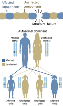
Only one mutated copy of the gene will be necessary for a person to be affected by an autosomal dominant disorder. Each affected person usually has one affected parent. The chance a child will inherit the mutated gene is 50%. Autosomal dominant conditions sometimes have reduced penetrance, which means although only one mutated copy is needed, not all individuals who inherit that mutation go on to develop the disease. Examples of this type of disorder are Huntington's disease, neurofibromatosis type 1, neurofibromatosis type 2, Marfan syndrome, hereditary nonpolyposis colorectal cancer, hereditary multiple exostoses (a highly penetrant autosomal dominant disorder), tuberous sclerosis, Von Willebrand disease, and acute intermittent porphyria. Birth defects are also called congenital anomalies.

Autosomal recessive

Main article: Autosomal dominant § Autosomal recessive allele

Two copies of the gene must be mutated for a person to be affected by an autosomal recessive disorder. An affected person usually has unaffected parents who each carry a single copy of the mutated gene and are referred to as genetic carriers. Each parent with a defective gene normally do not have symptoms. Two unaffected people who each carry one copy of the mutated gene have a 25% risk with each pregnancy of having a child affected by the disorder. Examples of this type of disorder are albinism, medium-chain acyl-CoA dehydrogenase deficiency, cystic fibrosis, sickle cell disease, Tay–Sachs disease, Niemann–Pick disease, spinal muscular atrophy, and Roberts syndrome. Certain other phenotypes, such as wet versus dry earwax, are also determined in an autosomal recessive fashion. Some autosomal recessive disorders are common because, in the past, carrying one of the faulty genes led to a slight protection against an infectious disease or toxin such as tuberculosis or malaria. Such disorders include cystic fibrosis, sickle cell disease, phenylketonuria and thalassaemia.

• 
  Hereditary defects in enzymes are generally inherited in an autosomal fashion because there are more non-X chromosomes than X-chromosomes, and a recessive fashion because the enzymes from the unaffected genes are generally sufficient to prevent symptoms in carriers.
  
  
• 
  On the other hand, hereditary defects in structural proteins (such as osteogenesis imperfecta, Marfan's syndrome and many Ehlers–Danlos syndromes) are generally autosomal dominant, because it is enough that some components are defective to make the whole structure dysfunctional. This is a dominant-negative process, wherein a mutated gene product adversely affects the non-mutated gene product within the same cell.

X-linked dominant

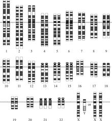
Schematic karyogram showing an overview of the human genome. It shows annotated bands and sub-bands as used in the nomenclature of genetic disorders. It shows 22 homologous chromosomes, both the female (XX) and male (XY) versions of the sex chromosome (bottom right), as well as the mitochondrial genome (to scale at bottom left).

Further information: Karyotype

Main article: X-linked dominant

X-linked dominant disorders are caused by mutations in genes on the X chromosome. Only a few disorders have this inheritance pattern, with a prime example being X-linked hypophosphatemic rickets. Males and females are both affected in these disorders, with males typically being more severely affected than females. Some X-linked dominant conditions, such as Rett syndrome, incontinentia pigmenti type 2, and Aicardi syndrome, are usually fatal in males either in utero or shortly after birth, and are therefore predominantly seen in females. Exceptions to this finding are extremely rare cases in which boys with Klinefelter syndrome (44+xxy) also inherit an X-linked dominant condition and exhibit symptoms more similar to those of a female in terms of disease severity. The chance of passing on an X-linked dominant disorder differs between men and women. The sons of a man with an X-linked dominant disorder will all be unaffected (since they receive their father's Y chromosome), but his daughters will all inherit the condition. A woman with an X-linked dominant disorder has a 50% chance of having an affected fetus with each pregnancy, although in cases such as incontinentia pigmenti, only female offspring are generally viable.

X-linked recessive

Main article: X-linked recessive inheritance

X-linked recessive conditions are also caused by mutations in genes on the X chromosome. Males are much more frequently affected than females, because they only have the one X chromosome necessary for the condition to present. The chance of passing on the disorder differs between men and women. The sons of a man with an X-linked recessive disorder will not be affected (since they receive their father's Y chromosome), but his daughters will be carriers of one copy of the mutated gene. A woman who is a carrier of an X-linked recessive disorder (X^RX^r) has a 50% chance of having sons who are affected and a 50% chance of having daughters who are carriers of one copy of the mutated gene. X-linked recessive conditions include the serious diseases hemophilia A, Duchenne muscular dystrophy, and Lesch–Nyhan syndrome, as well as common and less serious conditions such as male pattern baldness and red–green color blindness. X-linked recessive conditions can sometimes manifest in females due to skewed X-inactivation or monosomy X (Turner syndrome).

Y-linked

Main article: Y linkage

Y-linked disorders are caused by mutations on the Y chromosome. These conditions may only be transmitted from the heterogametic sex (e.g. male humans) to offspring of the same sex. More simply, this means that Y-linked disorders in humans can only be passed from men to their sons; females can never be affected because they do not possess Y-allosomes.

Y-linked disorders are exceedingly rare but the most well-known examples typically cause infertility. Reproduction in such conditions is only possible through the circumvention of infertility by medical intervention.

Mitochondrial

Main articles: Mitochondrial disease and Mitochondrial DNA

This type of inheritance, also known as maternal inheritance, is the rarest and applies to the 13 genes encoded by mitochondrial DNA. Because only egg cells contribute mitochondria to the developing embryo, only mothers (who are affected) can pass on mitochondrial DNA conditions to their children. An example of this type of disorder is Leber's hereditary optic neuropathy.

It is important to stress that the vast majority of mitochondrial diseases (particularly when symptoms develop in early life) are actually caused by a nuclear gene defect, as the mitochondria are mostly developed by non-mitochondrial DNA. These diseases most often follow autosomal recessive inheritance.

Multifactorial disorder

Main article: Multifactorial disease

Genetic disorders may also be complex, multifactorial, or polygenic, meaning they are likely associated with the effects of multiple genes in combination with lifestyles and environmental factors. Multifactorial disorders include heart disease and diabetes. Although complex disorders often cluster in families, they do not have a clear-cut pattern of inheritance. This makes it difficult to determine a person's risk of inheriting or passing on these disorders. Complex disorders are also difficult to study and treat because the specific factors that cause most of these disorders have not yet been identified. Studies that aim to identify the cause of complex disorders can use several methodological approaches to determine genotype–phenotype associations. One method, the genotype-first approach, starts by identifying genetic variants within patients and then determining the associated clinical manifestations. This is opposed to the more traditional phenotype-first approach, and may identify causal factors that have previously been obscured by clinical heterogeneity, penetrance, and expressivity.

On a pedigree, polygenic diseases do tend to "run in families", but the inheritance does not fit simple patterns as with Mendelian diseases. This does not mean that the genes cannot eventually be located and studied. There is also a strong environmental component to many of them (e.g., blood pressure). Other factors include:

• asthma
• autoimmune diseases such as multiple sclerosis
• cancers
• ciliopathies
• cleft palate
• diabetes
• heart disease
• hypertension
• inflammatory bowel disease
• intellectual disability
• mood disorder
• obesity
• refractive error
• infertility

Chromosomal disorder

See also: Chromosome abnormality

Chromosomes in Down syndrome, the most common human condition due to aneuploidy. There are three chromosomes 21 (in the last row).

A chromosomal disorder is a missing, extra, or irregular portion of chromosomal DNA. It can be from an atypical number of chromosomes or a structural abnormality in one or more chromosomes. An example of these disorders is Trisomy 21 (the most common form of Down syndrome), in which there is an extra copy of chromosome 21 in all cells.

Diagnosis

Due to the wide range of genetic disorders that are known, diagnosis is widely varied and dependent of the disorder. Most genetic disorders are diagnosed pre-birth, at birth, or during early childhood however some, such as Huntington's disease, can escape detection until the patient begins exhibiting symptoms well into adulthood.

The basic aspects of a genetic disorder rests on the inheritance of genetic material. With an in depth family history, it is possible to anticipate possible disorders in children which direct medical professionals to specific tests depending on the disorder and allow parents the chance to prepare for potential lifestyle changes, anticipate the possibility of stillbirth, or contemplate termination. Prenatal diagnosis can detect the presence of characteristic abnormalities in fetal development through ultrasound, or detect the presence of characteristic substances via invasive procedures which involve inserting probes or needles into the uterus such as in amniocentesis.

Prognosis

Not all genetic disorders directly result in death; however, there are no known cures for genetic disorders. Many genetic disorders affect stages of development, such as Down syndrome, while others result in purely physical symptoms such as muscular dystrophy. Other disorders, such as Huntington's disease, show no signs until adulthood. During the active time of a genetic disorder, patients mostly rely on maintaining or slowing the degradation of quality of life and maintain patient autonomy. This includes physical therapy and pain management.

Treatment

From personal genomics to gene therapy

See also: Gene therapy

The treatment of genetic disorders is an ongoing battle, with over 1,800 gene therapy clinical trials having been completed, are ongoing, or have been approved worldwide. Despite this, most treatment options revolve around treating the symptoms of the disorders in an attempt to improve patient quality of life.

Gene therapy refers to a form of treatment where a healthy gene is introduced to a patient. This should alleviate the defect caused by a faulty gene or slow the progression of the disease. A major obstacle has been the delivery of genes to the appropriate cell, tissue, and organ affected by the disorder. Researchers have investigated how they can introduce a gene into the potentially trillions of cells that carry the defective copy. Finding an answer to this has been a roadblock between understanding the genetic disorder and correcting the genetic disorder.

Epidemiology

Around 1 in 50 people are affected by a known single-gene disorder, while around 1 in 263 are affected by a chromosomal disorder. Around 65% of people have some kind of health problem as a result of congenital genetic mutations. Due to the significantly large number of genetic disorders, approximately 1 in 21 people are affected by a genetic disorder classified as "rare" (usually defined as affecting less than 1 in 2,000 people). Most genetic disorders are rare in themselves. There are well over 6,000 known genetic disorders, and new genetic disorders are constantly being described in medical literature.

History

The earliest known genetic condition in a hominid was in the fossil species Paranthropus robustus, with over a third of individuals displaying amelogenesis imperfecta.

Transmutation of species

The Transmutation of species and transformism are 18th and early 19th-century ideas about the change of one species into another that preceded Charles Darwin's theory of evolution through natural selection. The French Transformisme was a term used by Jean Baptiste Lamarck in 1809 for his theory, and other 18th and 19th century proponents of pre-Darwinian evolutionary ideas included Denis Diderot, Étienne Geoffroy Saint-Hilaire, Erasmus Darwin, Robert Grant, and Robert Chambers, the anonymous author of the book Vestiges of the Natural History of Creation. Such ideas were associated with 18th century ideas of Deism and human progress. Opposition in the scientific community to these early theories of evolution, led by influential scientists like the anatomists Georges Cuvier and Richard Owen, and the geologist Charles Lyell, was intense. The debate over them was an important stage in the history of evolutionary thought and influenced the subsequent reaction to Darwin's theory.

Terminology

Transmutation was one of the names commonly used for evolutionary ideas in the 19th century before Charles Darwin published On The Origin of Species (1859). Transmutation had previously been used as a term in alchemy to describe the transformation of base metals into gold. Other names for evolutionary ideas used in this period include the development hypothesis (one of the terms used by Darwin) and the theory of regular gradation, used by William Chilton in the periodical press such as The Oracle of Reason. Transformation is another word used quite as often as transmutation in this context. These early 19th century evolutionary ideas played an important role in the history of evolutionary thought.

The proto-evolutionary thinkers of the 18th and early 19th century had to invent terms to label their ideas, but it was first Joseph Gottlieb Kölreuter who used the term "transmutation" to refer to species who have had biological changes through hybridization.

The terminology did not settle down until some time after the publication of the Origin of Species. The word evolved in a modern sense was first used in 1826 in an anonymous paper published in Robert Jameson's journal and evolution was a relative late-comer which can be seen in Herbert Spencer's Social Statics of 1851, and at least one earlier example, but was not in general use until about 1865–70.

Historical development

Ideas before the 18th century

In the 10th and 11th centuries, Ibn Miskawayh's Al-Fawz al-Kabir (الفوز الأكبر), and the Brethren of Purity's Encyclopedia of the Brethren of Purity (رسائل إخوان الصفا‎) developed ideas about changes in biological species. In 1993, Muhammad Hamidullah described the ideas in lectures:

[These books] state that God first created matter and invested it with energy for development. Matter, therefore, adopted the form of vapour which assumed the shape of water in due time. The next stage of development was mineral life. Different kinds of stones developed in course of time. Their highest form being mirjan (coral). It is a stone which has in it branches like those of a tree. After mineral life evolves vegetation. The evolution of vegetation culminates with a tree which bears the qualities of an animal. This is the date-palm. It has male and female genders. It does not wither if all its branches are chopped but it dies when the head is cut off. The date-palm is therefore considered the highest among the trees and resembles the lowest among animals. Then is born the lowest of animals. It evolves into an ape. This is not the statement of Darwin. This is what Ibn Maskawayh states and this is precisely what is written in the Epistles of Ikhwan al-Safa. The Muslim thinkers state that ape then evolved into a lower kind of a barbarian man. He then became a superior human being. Man becomes a saint, a prophet. He evolves into a higher stage and becomes an angel. The one higher to angels is indeed none but God. Everything begins from Him and everything returns to Him.

In the 14th century, Ibn Khaldun further developed these ideas. According to some commentators, statements in his 1377 work, the Muqaddimah anticipate the biological theory of evolution.

Robert Hooke proposed in a speech to the Royal Society in the late 17th century that species vary, change, and especially become extinct. His “Discourse of Earthquakes” was based on comparisons made between fossils, especially the modern pearly nautilus and the curled shells of ammonites.

18th and early 19th century

In the 18th century, Jacques-Antoine des Bureaux claimed a "genealogical ascent of species". He argued that through crossbreeding and hybridization in reproduction, "progressive organization" occurred, allowing organisms to change and more complex species to develop.

Simultaneously, Retif de la Bretonne wrote La decouverte australe par un homme-volant (1781) and La philosophie de monsieur Nicolas (1796), which encapsulated his view that more complex species, such as mankind, had developed step-by-step from "less perfect" animals. De la Bretonne believed that living forms undergo constant change. Although he believed in constant change, he took a very different approach from Diderot: chance and blind combinations of atoms, in de la Bretonne's opinion, were not the cause of transmutation. De la Bretonne argued that all species had developed from more primitive organisms, and that nature aimed to reach perfection.

Denis Diderot, chief editor of the Encyclopédie, spent his time poring over scientific theories attempting to explain rock strata and the diversity of fossils. Geological and fossil evidence was presented to him as contributions to Encyclopedia articles, chief among them "Mammoth", "Fossil", and "Ivory Fossil", all of which noted the existence of mammoth bones in Siberia. As a result of this geological and fossil evidence, Diderot believed that species were mutable. Particularly, he argued that organisms metamorphosized over millennia, resulting in species changes. In Diderot's theory of transformationism, random chance plays a large role in allowing species to change, develop and become extinct, as well as having new species form. Specifically, Diderot believed that given randomness and an infinite number of times, all possible scenarios would manifest themselves. He proposed that this randomness was behind the development of new traits in offspring and as a result the development and extinction of species.

Diderot drew from Leonardo da Vinci’s comparison of the leg structure of a human and a horse as proof of the interconnectivity of species. He saw this experiment as demonstrating that nature could continually try out new variations. Additionally, Diderot argued that organic molecules and organic matter possessed an inherent consciousness, which allowed the smallest particles of organic matter to organize into fibers, then a network, and then organs. The idea that organic molecules have consciousness was derived from both Maupertuis and Lucretian texts. Overall, Diderot’s musings all fit together as a "composite transformist philosophy", one dependent on the randomness inherent to nature as a transformist mechanism.

Erasmus Darwin

Erasmus Darwin developed a theory of universal transformation. His major works, The Botanic Garden (1792), Zoonomia (1794–96), and The Temple of Nature all touched on the transformation of organic creatures. In both The Botanic Garden and The Temple of Nature, Darwin used poetry to describe his ideas regarding species. In Zoonomia, however, Erasmus clearly articulates (as a more scientific text) his beliefs about the connections between organic life. He notes particularly that some plants and animals have "useless appendages", which have gradually changed from their original, useful states. Additionally, Darwin relied on cosmological transformation as a crucial aspect of his theory of transformation, making a connection between William Herschel’s approach to natural historical cosmology and the changing aspects of plants and animals.

Erasmus believed that life had one origin, a common ancestor, which he referred to as the "filament" of life. He used his understanding of chemical transmutation to justify the spontaneous generation of this filament. His geological study of Derbyshire and the sea- shells and fossils which he found there helped him to come to the conclusion that complex life had developed from more primitive forms (Laniel-Musitelli). Erasmus was an early proponent of what we now refer to as "adaptations", albeit through a different transformist mechanism – he argued that sexual reproduction could pass on acquired traits through the father’s contribution to the embryon. These changes, he believed, were mainly driven by the three great needs of life: lust, food, and security. Erasmus proposed that these acquired changes gradually altered the physical makeup of organisms as a result of the desires of plants and animals. Notably, he describes insects developing from plants, a grand example of one species transforming into another.

Erasmus Darwin relied on Lucretian philosophy to form a theory of universal change. He proposed that both organic and inorganic matter changed throughout the course of the universe, and that plants and animals could pass on acquired traits to their progeny. His view of universal transformation placed time as a driving force in the universe’s journey towards improvement. In addition, Erasmus believed that nature had some amount of agency in this inheritance. Darwin spun his own story of how nature began to develop from the ocean, and then slowly became more diverse and more complex. His transmutation theory relied heavily on the needs which drove animal competition, as well as the results of this contest between both animals and plants.

Charles Darwin acknowledged his grandfather’s contribution to the field of transmutation in his synopsis of Erasmus’ life, The Life of Erasmus Darwin. Darwin collaborated with Ernst Krause to write a forward on Krause's Erasmus Darwin und Seine Stellung in Der Geschichte Der Descendenz-Theorie, which translates into Erasmus Darwin and His Place in the History of the Descent Theory. Krause explains Erasmus' motivations for arguing for the theory of descent, including Darwin's connection with and correspondence with Rousseau, which may have influenced how he saw the world.

Lamarck

See also: Lamarckism

Jean-Baptiste Lamarck proposed a hypothesis on the transmutation of species in Philosophie Zoologique (1809). Lamarck did not believe that all living things shared a common ancestor. Rather he believed that simple forms of life were created continuously by spontaneous generation. He also believed that an innate life force, which he sometimes described as a nervous fluid, drove species to become more complex over time, advancing up a linear ladder of complexity that was related to the great chain of being. Lamarck also recognized that species were adapted to their environment. He explained this observation by saying that the same nervous fluid driving increasing complexity, also caused the organs of an animal (or a plant) to change based on the use or disuse of that organ, just as muscles are affected by exercise. He argued that these changes would be inherited by the next generation and produce slow adaptation to the environment. It was this secondary mechanism of adaptation through the inheritance of acquired characteristics that became closely associated with his name and would influence discussions of evolution into the 20th century.

Ideas after Lamarck

The German Abraham Gottlob Werner believed in geological transformism. Specifically, Werner argued that the Earth undergoes irreversible and continuous change. The Edinburgh school, a radical British school of comparative anatomy, fostered a lot of debate around natural history. Edinburgh, which included the surgeon Robert Knox and the anatomist Robert Grant, was closely in touch with Lamarck's school of French Transformationism, which contained scientists such as Étienne Geoffroy Saint-Hilaire. Grant developed Lamarck's and Erasmus Darwin's ideas of transmutation and evolutionism, investigating homology to prove common descent. As a young student Charles Darwin joined Grant in investigations of the life cycle of marine animals. He also studied geology under professor Robert Jameson whose journal published an anonymous paper in 1826 praising "Mr. Lamarck" for explaining how the higher animals had "evolved" from the "simplest worms" – this was the first use of the word "evolved" in a modern sense. Professor Jameson was a Wernerian, which allowed him to consider transformation theories and foster the interest in transformism among his students. Jameson's course closed with lectures on the "Origin of the Species of Animals".

Vestiges of the Natural History of Creation

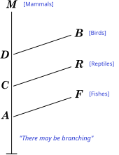
Diagram from the 1844 book Vestiges of the Natural History of Creation by Robert Chambers shows a model of development where fishes (F), reptiles (R), and birds (B) represent branches from a path leading to mammals (M).

The computing pioneer Charles Babbage published his unofficial Ninth Bridgewater Treatise in 1837, putting forward the thesis that God had the omnipotence and foresight to create as a divine legislator, making laws (or programs) which then produced species at the appropriate times, rather than continually interfering with ad hoc miracles each time a new species was required. In 1844 the Scottish publisher Robert Chambers anonymously published an influential and extremely controversial book of popular science entitled Vestiges of the Natural History of Creation. This book proposed an evolutionary scenario for the origins of the solar system and life on earth. It claimed that the fossil record showed an ascent of animals with current animals being branches off a main line that leads progressively to humanity. It implied that the transmutations led to the unfolding of a preordained orthogenetic plan woven into the laws that governed the universe. In this sense it was less completely materialistic than the ideas of radicals like Robert Grant, but its implication that humans were just the last step in the ascent of animal life incensed many conservative thinkers. Both conservatives like Adam Sedgwick, and radical materialists like Thomas Henry Huxley, who disliked Chambers' implications of preordained progress, were able to find scientific inaccuracies in the book that they could disparage. Darwin himself openly deplored the author's "poverty of intellect", and dismissed it as a "literary curiosity". However, the high profile of the public debate over Vestiges, with its depiction of evolution as a progressive process, and its popular success, would greatly influence the perception of Darwin's theory a decade later. It also influenced some younger naturalists, including Alfred Russel Wallace, to take an interest in the idea of transmutation.

Ideological motivations for theories of transmutation

The proponents of transmutation were almost all inclined to Deism—the idea, popular among many 18th century Western intellectuals that God had initially created the universe, but then left it to operate and develop through natural law rather than through divine intervention. Thinkers like Erasmus Darwin saw the transmutation of species as part of this development of the world through natural law, which they saw as a challenge to traditional Christianity. They also believed that human history was progressive, which was another idea becoming increasingly popular in the 18th century. They saw progress in human history as being mirrored by the development of life from the simple to the complex over the history of the Earth. This connection was very clear in the work of Erasmus Darwin and Robert Chambers.

Opposition to transmutation

Ideas about the transmutation of species were strongly associated with the anti-Christen materialism and radical political ideas of the Enlightenment and were greeted with hostility by more conservative thinkers. Cuvier attacked the ideas of Lamarck and Geoffroy Saint-Hilaire, agreeing with Aristotle that species were immutable. Cuvier believed that the individual parts of an animal were too closely correlated with one another to allow for one part of the anatomy to change in isolation from the others, and argued that the fossil record showed patterns of catastrophic extinctions followed by re-population, rather than gradual change over time. He also noted that drawings of animals and animal mummies from Egypt, which were thousands of years old, showed no signs of change when compared with modern animals. The strength of Cuvier's arguments and his reputation as a leading scientist helped keep transmutational ideas out of the scientific mainstream for decades.

In Britain, where the philosophy of natural theology remained influential, William Paley wrote the book Natural Theology with its famous watchmaker analogy, at least in part as a response to the transmutational ideas of Erasmus Darwin. Geologists influenced by natural theology, such as Buckland and Sedgwick, made a regular practice of attacking the evolutionary ideas of Lamarck and Grant, and Sedgwick wrote a famously harsh review of The Vestiges of the Natural History of Creation. Although the geologist Charles Lyell opposed scriptural geology, he also believed in the immutability of species, and in his Principles of Geology (1830–1833) he criticized and dismissed Lamarck's theories of development. Instead, he advocated a form of progressive creation, in which each species had its "centre of creation" and was designed for this particular habitat, but would go extinct when this habitat changed.

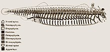
This 1847 diagram by Richard Owen shows his conceptual archetype for all vertebrates.

Another source of opposition to transmutation was a school of naturalists who were influenced by the German philosophers and naturalists associated with idealism, such as Goethe, Hegel and Lorenz Oken. Idealists such as Louis Agassiz and Richard Owen believed that each species was fixed and unchangeable because it represented an idea in the mind of the creator. They believed that relationships between species could be discerned from developmental patterns in embryology, as well as in the fossil record, but that these relationships represented an underlying pattern of divine thought, with progressive creation leading to increasing complexity and culminating in humanity. Owen developed the idea of "archetypes" in the divine mind that would produce a sequence of species related by anatomical homologies, such as vertebrate limbs. Owen was concerned by the political implications of the ideas of transmutationists like Robert Grant, and he led a public campaign by conservatives that successfully marginalized Grant in the scientific community. In his famous 1841 paper, which coined the term dinosaur for the giant reptiles discovered by Buckland and Gideon Mantell, Owen argued that these reptiles contradicted the transmutational ideas of Lamarck because they were more sophisticated than the reptiles of the modern world. Darwin would make good use of the homologies analyzed by Owen in his own theory, but the harsh treatment of Grant, along with the controversy surrounding Vestiges, would be factors in his decision to ensure that his theory was fully supported by facts and arguments before publishing his ideas.

Evolution of biological complexity

From Wikipedia, the free encyclopedia
https://en.wikipedia.org/wiki/Evolution_of_biological_complexity

The evolution of biological complexity is one important outcome of the process of evolution. Evolution has produced some remarkably complex organisms – although the actual level of complexity is very hard to define or measure accurately in biology, with properties such as gene content, the number of cell types or morphology all proposed as possible metrics.

Many biologists used to believe that evolution was progressive (orthogenesis) and had a direction that led towards so-called "higher organisms", despite a lack of evidence for this viewpoint. This idea of "progression" introduced the terms "high animals" and "low animals" in evolution. Many now regard this as misleading, with natural selection having no intrinsic direction and that organisms selected for either increased or decreased complexity in response to local environmental conditions. Although there has been an increase in the maximum level of complexity over the history of life, there has always been a large majority of small and simple organisms and the most common level of complexity appears to have remained relatively constant.

Selection for simplicity and complexity

Usually organisms that have a higher rate of reproduction than their competitors have an evolutionary advantage. Consequently, organisms can evolve to become simpler and thus multiply faster and produce more offspring, as they require fewer resources to reproduce. A good example are parasites such as Plasmodium – the parasite responsible for malaria – and mycoplasma; these organisms often dispense with traits that are made unnecessary through parasitism on a host.

A lineage can also dispense with complexity when a particular complex trait merely provides no selective advantage in a particular environment. Loss of this trait need not necessarily confer a selective advantage, but may be lost due to the accumulation of mutations if its loss does not confer an immediate selective disadvantage. For example, a parasitic organism may dispense with the synthetic pathway of a metabolite where it can readily scavenge that metabolite from its host. Discarding this synthesis may not necessarily allow the parasite to conserve significant energy or resources and grow faster, but the loss may be fixed in the population through mutation accumulation if no disadvantage is incurred by loss of that pathway. Mutations causing loss of a complex trait occur more often than mutations causing gain of a complex trait.

With selection, evolution can also produce more complex organisms. Complexity often arises in the co-evolution of hosts and pathogens, with each side developing ever more sophisticated adaptations, such as the immune system and the many techniques pathogens have developed to evade it. For example, the parasite Trypanosoma brucei, which causes sleeping sickness, has evolved so many copies of its major surface antigen that about 10% of its genome is devoted to different versions of this one gene. This tremendous complexity allows the parasite to constantly change its surface and thus evade the immune system through antigenic variation.

More generally, the growth of complexity may be driven by the co-evolution between an organism and the ecosystem of predators, prey and parasites to which it tries to stay adapted: as any of these become more complex in order to cope better with the diversity of threats offered by the ecosystem formed by the others, the others too will have to adapt by becoming more complex, thus triggering an ongoing evolutionary arms race towards more complexity. This trend may be reinforced by the fact that ecosystems themselves tend to become more complex over time, as species diversity increases, together with the linkages or dependencies between species.

Types of trends in complexity

Passive versus active trends in complexity. Organisms at the beginning are red. Numbers are shown by height with time moving up in a series.

If evolution possessed an active trend toward complexity (orthogenesis), as was widely believed in the 19th century, then we would expect to see an active trend of increase over time in the most common value (the mode) of complexity among organisms.

However, an increase in complexity can also be explained through a passive process. Assuming unbiased random changes of complexity and the existence of a minimum complexity leads to an increase over time of the average complexity of the biosphere. This involves an increase in variance, but the mode does not change. The trend towards the creation of some organisms with higher complexity over time exists, but it involves increasingly small percentages of living things.

In this hypothesis, any appearance of evolution acting with an intrinsic direction towards increasingly complex organisms is a result of people concentrating on the small number of large, complex organisms that inhabit the right-hand tail of the complexity distribution and ignoring simpler and much more common organisms. This passive model predicts that the majority of species are microscopic prokaryotes, which is supported by estimates of 10⁶ to 10⁹ extant prokaryotes compared to diversity estimates of 10⁶ to 3·10⁶ for eukaryotes. Consequently, in this view, microscopic life dominates Earth, and large organisms only appear more diverse due to sampling bias.

Genome complexity has generally increased since the beginning of the life on Earth. Some computer models have suggested that the generation of complex organisms is an inescapable feature of evolution. Proteins tend to become more hydrophobic over time, and to have their hydrophobic amino acids more interspersed along the primary sequence. Increases in body size over time are sometimes seen in what is known as Cope's rule.

Constructive neutral evolution

Further information: Constructive neutral evolution

Recently work in evolution theory has proposed that by relaxing selection pressure, which typically acts to streamline genomes, the complexity of an organism increases by a process called constructive neutral evolution. Since the effective population size in eukaryotes (especially multi-cellular organisms) is much smaller than in prokaryotes, they experience lower selection constraints.

According to this model, new genes are created by non-adaptive processes, such as by random gene duplication. These novel entities, although not required for viability, do give the organism excess capacity that can facilitate the mutational decay of functional subunits. If this decay results in a situation where all of the genes are now required, the organism has been trapped in a new state where the number of genes has increased. This process has been sometimes described as a complexifying ratchet. These supplemental genes can then be co-opted by natural selection by a process called neofunctionalization. In other instances constructive neutral evolution does not promote the creation of new parts, but rather promotes novel interactions between existing players, which then take on new moonlighting roles.

Constructive neutral evolution has also been used to explain how ancient complexes, such as the spliceosome and the ribosome, have gained new subunits over time, how new alternative spliced isoforms of genes arise, how gene scrambling in ciliates evolved, how pervasive pan-RNA editing may have arisen in Trypanosoma brucei, how functional lncRNAs have likely arisen from transcriptional noise, and how even useless protein complexes can persist for millions of years.

Mutational hazard hypothesis

The mutational hazard hypothesis is a non-adaptive theory for increased complexity in genomes. The basis of mutational hazard hypothesis is that each mutation for non-coding DNA imposes a fitness cost. Variation in complexity can be described by 2N_eu, where N_e is effective population size and u is mutation rate.

In this hypothesis, selection against non-coding DNA can be reduced in three ways: random genetic drift, recombination rate, and mutation rate. As complexity increases from prokaryotes to multicellular eukaryotes, effective population size decreases, subsequently increasing the strength of random genetic drift. This, along with low recombination rate and high mutation rate, allows non-coding DNA to proliferate without being removed by purifying selection.

Accumulation of non-coding DNA in larger genomes can be seen when comparing genome size and genome content across eukaryotic taxa. There is a positive correlation between genome size and noncoding DNA genome content with each group staying within some variation. When comparing variation in complexity in organelles, effective population size is replaced with genetic effective population size (N_g). If looking at silent-site nucleotide diversity, then larger genomes are expected to have less diversity than more compact ones. In plant and animal mitochondria, differences in mutation rate account for the opposite directions in complexity, with plant mitochondria being more complex and animal mitochondria more streamlined.

The mutational hazard hypothesis has been used to at least partially explain expanded genomes in some species. For example, when comparing Volvox cateri to a close relative with a compact genome, Chlamydomonas reinhardtii, the former had less silent-site diversity than the latter in nuclear, mitochondrial, and plastid genomes. However when comparing the plastid genome of Volvox cateri to Volvox africanus, a species in the same genus but with half the plastid genome size, there was high mutation rates in intergenic regions. In Arabiopsis thaliana, the hypothesis was used as a possible explanation for intron loss and compact genome size. When compared to Arabidopsis lyrata, researchers found a higher mutation rate overall and in lost introns (an intron that is no longer transcribed or spliced) compared to conserved introns.

There are expanded genomes in other species that could not be explained by the mutational hazard hypothesis. For example, the expanded mitochondrial genomes of Silene noctiflora and Silene conica have high mutation rates, lower intron lengths, and more non-coding DNA elements compared to others in the same genus, but there was no evidence for long-term low effective population size. The mitochondrial genomes of Citrullus lanatus and Cucurbita pepo differ in several ways. Citrullus lanatus is smaller, has more introns and duplications, while Cucurbita pepo is larger with more chloroplast and short repeated sequences. If RNA editing sites and mutation rate lined up, then Cucurbita pepo would have a lower mutation rate and more RNA editing sites. However the mutation rate is four times higher than Citrullus lanatus and they have a similar number of RNA editing sites. There was also an attempt to use the hypothesis to explain large nuclear genomes of salamanders, but researchers found opposite results than expected, including lower long-term strength of genetic drift.

History

Further information: Orthogenesis

In the 19th century, some scientists such as Jean-Baptiste Lamarck (1744–1829) and Ray Lankester (1847–1929) believed that nature had an innate striving to become more complex with evolution. This belief may reflect then-current ideas of Hegel (1770–1831) and of Herbert Spencer (1820–1903) which envisaged the universe gradually evolving to a higher, more perfect state.

This view regarded the evolution of parasites from independent organisms to a parasitic species as "devolution" or "degeneration", and contrary to nature. Social theorists have sometimes interpreted this approach metaphorically to decry certain categories of people as "degenerate parasites". Later scientists regarded biological devolution as nonsense; rather, lineages become simpler or more complicated according to whatever forms had a selective advantage.

In a 1964 book, The Emergence of Biological Organization, Quastler pioneered a theory of emergence, developing a model of a series of emergences from protobiological systems to prokaryotes without the need to invoke implausible very low probability events.

The evolution of order, manifested as biological complexity, in living systems and the generation of order in certain non-living systems was proposed in 1983 to obey a common fundamental principal called “the Darwinian dynamic”. The Darwinian dynamic was formulated by first considering how microscopic order is generated in simple non-biological systems that are far from thermodynamic equilibrium. Consideration was then extended to short, replicating RNA molecules assumed to be similar to the earliest forms of life in the RNA world. It was shown that the underlying order-generating processes in the non-biological systems and in replicating RNA are basically similar. This approach helped clarify the relationship of thermodynamics to evolution as well as the empirical content of Darwin's theory.

In 1985, Morowitz noted that the modern era of irreversible thermodynamics ushered in by Lars Onsager in the 1930s showed that systems invariably become ordered under a flow of energy, thus indicating that the existence of life involves no contradiction to the laws of physics.