Search This Blog

Sunday, November 22, 2020

Attribution of recent climate change

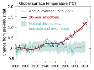
Observed temperature from NASA vs the 1850–1900 average used by the IPCC as a pre-industrial baseline. The primary driver for increased global temperatures in the industrial era is human activity, with natural forces adding variability.

Attribution of recent climate change is the effort to scientifically ascertain mechanisms responsible for recent global warming and related climate changes on Earth. The effort has focused on changes observed during the period of instrumental temperature record, particularly in the last 50 years. This is the period when human activity has grown fastest and observations of the atmosphere above the surface have become available. According to the Intergovernmental Panel on Climate Change (IPCC), it is "extremely likely" that human influence was the dominant cause of global warming between 1951 and 2010. Likely human contribution is 93%–123% of the observed 1951–2010 temperature change.

Some of the main human activities that contribute to global warming are:

Probability density function (PDF) of fraction of surface temperature trends since 1950 attributable to human activity, based on IPCC AR5 10.5

In addition to human activities, some natural mechanisms can also cause climate change, including for example, climate oscillations, changes in solar activity, and volcanic activity.

Multiple lines of evidence support attribution of recent climate change to human activities:

  • A physical understanding of the climate system: greenhouse gas concentrations have increased and their warming properties are well-established.
  • Historical estimates of past climate changes suggest that the recent changes in global surface temperature are unusual.
  • Computer-based climate models are unable to replicate the observed warming unless human greenhouse gas emissions are included.
  • Natural forces alone (such as solar and volcanic activity) cannot explain the observed warming.

The IPCC's attribution of recent global warming to human activities is a view shared by the scientific community, and is also supported by 196 other scientific organizations worldwide.

Background

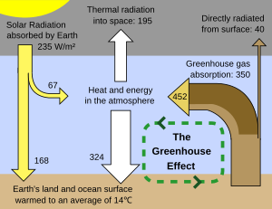
Energy flows between space, the atmosphere, and Earth's surface. Current greenhouse gas levels are causing a radiative imbalance of about 0.9 W/m2.

Factors affecting Earth's climate can be broken down into feedbacks and forcings. A forcing is something that is imposed externally on the climate system. External forcings include natural phenomena such as volcanic eruptions and variations in the sun's output. Human activities can also impose forcings, for example, through changing the composition of the atmosphere.

Radiative forcing is a measure of how various factors alter the energy balance of the Earth's atmosphere. A positive radiative forcing will tend to increase the energy of the Earth-atmosphere system, leading to a warming of the system. Between the start of the Industrial Revolution in 1750, and the year 2005, the increase in the atmospheric concentration of carbon dioxide (chemical formula: CO
2
) led to a positive radiative forcing, averaged over the Earth's surface area, of about 1.66 watts per square metre (abbreviated W m−2).

Climate feedbacks can either amplify or dampen the response of the climate to a given forcing. There are many feedback mechanisms in the climate system that can either amplify (a positive feedback) or diminish (a negative feedback) the effects of a change in climate forcing.

The climate system will vary in response to changes in forcings. The climate system will show internal variability both in the presence and absence of forcings imposed on it, (see images opposite). This internal variability is a result of complex interactions between components of the climate system, such as the coupling between the atmosphere and ocean (see also the later section on Internal climate variability and global warming). An example of internal variability is the El Niño–Southern Oscillation.

Detection vs. attribution

In detection and attribution, natural factors include changes in the Sun's output and volcanic eruptions, as well as natural modes of variability such as El Niño and La Niña. Human factors include the emissions of heat-trapping "greenhouse" gases and particulates as well as clearing of forests and other land-use changes. Figure source: NOAA NCDC.

Detection and attribution of climate signals, as well as its common-sense meaning, has a more precise definition within the climate change literature, as expressed by the IPCC. Detection of a climate signal does not always imply significant attribution. The IPCC's Fourth Assessment Report says "it is extremely likely that human activities have exerted a substantial net warming influence on climate since 1750," where "extremely likely" indicates a probability greater than 95%. Detection of a signal requires demonstrating that an observed change is statistically significantly different from that which can be explained by natural internal variability.

Attribution requires demonstrating that a signal is:

  • unlikely to be due entirely to internal variability;
  • consistent with the estimated responses to the given combination of anthropogenic and natural forcing
  • not consistent with alternative, physically plausible explanations of recent climate change that exclude important elements of the given combination of forcings.

Key attributions

Greenhouse gases

Radiative forcing of different contributors to climate change in 2011, as reported in the fifth IPCC assessment report.

Carbon dioxide is the primary greenhouse gas that is contributing to recent climate change. CO
2
is absorbed and emitted naturally as part of the carbon cycle, through animal and plant respiration, volcanic eruptions, and ocean-atmosphere exchange. Human activities, such as the burning of fossil fuels and changes in land use (see below), release large amounts of carbon to the atmosphere, causing CO
2
concentrations in the atmosphere to rise.

The high-accuracy measurements of atmospheric CO
2
concentration, initiated by Charles David Keeling in 1958, constitute the master time series documenting the changing composition of the atmosphere. These data have iconic status in climate change science as evidence of the effect of human activities on the chemical composition of the global atmosphere.

In May 2019, the concentration of CO
2
in the atmosphere reached 415 ppm. The last time when it reached this level was 2.6–5.3 million years ago. Without human intervention, it would be 280 ppm.

Along with CO
2
, methane and to a lesser extent nitrous oxide are also major forcing contributors to the greenhouse effect. The Kyoto Protocol lists these together with hydrofluorocarbon (HFCs), perfluorocarbons (PFCs), and sulfur hexafluoride (SF6), which are entirely artificial gases, as contributors to radiative forcing. The chart at right attributes anthropogenic greenhouse gas emissions to eight main economic sectors, of which the largest contributors are power stations (many of which burn coal or other fossil fuels), industrial processes, transportation fuels (generally fossil fuels), and agricultural by-products (mainly methane from enteric fermentation and nitrous oxide from fertilizer use).

Water vapor

Water vapor is the most abundant greenhouse gas and is the largest contributor to the natural greenhouse effect, despite having a short atmospheric lifetime (about 10 days). Some human activities can influence local water vapor levels. However, on a global scale, the concentration of water vapor is controlled by temperature, which influences overall rates of evaporation and precipitation. Therefore, the global concentration of water vapor is not substantially affected by direct human emissions.

Land use

Climate change is attributed to land use for two main reasons. Between 1750 and 2007, about two-thirds of anthropogenic CO
2
emissions were produced from burning fossil fuels, and about one-third of emissions from changes in land use, primarily deforestation. Deforestation both reduces the amount of carbon dioxide absorbed by deforested regions and releases greenhouse gases directly, together with aerosols, through biomass burning that frequently accompanies it.

Some of the causes of climate change are, generally, not connected with it directly in the media coverage. For example, the harm done by humans to the populations of Elephants and Monkeys contributes to deforestation therefore to climate change.

A second reason that climate change has been attributed to land use is that the terrestrial albedo is often altered by use, which leads to radiative forcing. This effect is more significant locally than globally.

Livestock and land use

Worldwide, livestock production occupies 70% of all land used for agriculture, or 30% of the ice-free land surface of the Earth. More than 18% of anthropogenic greenhouse gas emissions are attributed to livestock and livestock-related activities such as deforestation and increasingly fuel-intensive farming practices. Specific attributions to the livestock sector include:

Aerosols

With virtual certainty, scientific consensus has attributed various forms of climate change, chiefly cooling effects, to aerosols, which are small particles or droplets suspended in the atmosphere. Key sources to which anthropogenic aerosols are attributed include:

Attribution of 20th-century climate change

The Keeling Curve shows the long-term increase of atmospheric carbon dioxide (CO
2
) concentrations from 1958–2018. Monthly CO
2
measurements display seasonal oscillations in an upward trend. Each year's maximum occurs during the Northern Hemisphere's late spring.
 
CO
2
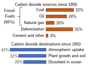
sources and sinks since 1880. While there is little debate that excess carbon dioxide in the industrial era has mostly come from burning fossil fuels, the future strength of land and ocean carbon sinks is an area of study.
 
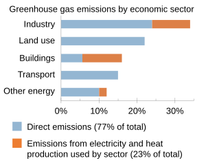
Contribution to climate change broken down by economic sectors, according to the IPCC AR5 report.

Over the past 150 years human activities have released increasing quantities of greenhouse gases into the atmosphere. This has led to increases in mean global temperature, or global warming. Other human effects are relevant—for example, sulphate aerosols are believed to have a cooling effect. Natural factors also contribute. According to the historical temperature record of the last century, the Earth's near-surface air temperature has risen around 0.74 ± 0.18 °Celsius (1.3 ± 0.32 °Fahrenheit).

A historically important question in climate change research has regarded the relative importance of human activity and non-anthropogenic causes during the period of instrumental record. In the 1995 Second Assessment Report (SAR), the IPCC made the widely quoted statement that "The balance of evidence suggests a discernible human influence on global climate". The phrase "balance of evidence" suggested the (English) common-law standard of proof required in civil as opposed to criminal courts: not as high as "beyond reasonable doubt". In 2001 the Third Assessment Report (TAR) refined this, saying "There is new and stronger evidence that most of the warming observed over the last 50 years is attributable to human activities". The 2007 Fourth Assessment Report (AR4) strengthened this finding:

  • "Anthropogenic warming of the climate system is widespread and can be detected in temperature observations taken at the surface, in the free atmosphere and in the oceans. Evidence of the effect of external influences, both anthropogenic and natural, on the climate system has continued to accumulate since the TAR."

Other findings of the IPCC Fourth Assessment Report include:

  • "It is extremely unlikely (<5%) that the global pattern of warming during the past half century can be explained without external forcing (i.e., it is inconsistent with being the result of internal variability), and very unlikely that it is due to known natural external causes alone. The warming occurred in both the ocean and the atmosphere and took place at a time when natural external forcing factors would likely have produced cooling."
  • "From new estimates of the combined anthropogenic forcing due to greenhouse gases, aerosols, and land surface changes, it is extremely likely (>95%) that human activities have exerted a substantial net warming influence on climate since 1750."
  • "It is virtually certain that anthropogenic aerosols produce a net negative radiative forcing (cooling influence) with a greater magnitude in the Northern Hemisphere than in the Southern Hemisphere."

Over the past five decades there has been a global warming of approximately 0.65 °C (1.17 °F) at the Earth's surface (see historical temperature r

In paleoanthropology, the recent African origin of modern humans, also called the "Out of Africa" theory (OOA), recent single-origin hypothesis (RSOH), replacement hypothesis, or recent African origin model (RAO), is the dominant model of the geographic origin and early migration of anatomically modern humans (Homo sapiens). It follows the early expansions of hominins out of Africa, accomplished by Homo erectus and then Homo neanderthalensis.

The model proposes a "single origin" of Homo sapiens in the taxonomic sense, precluding parallel evolution of traits considered anatomically modern in other regions, but not precluding multiple admixture between H. sapiens and archaic humans in Europe and Asia. H. sapiens most likely developed in the Horn of Africa between 300,000 and 200,000 years ago. The "recent African origin" model proposes that all modern non-African populations are substantially descended from populations of H. sapiens that left Africa after that time.

There were at least several "out-of-Africa" dispersals of modern humans, possibly beginning as early as 270,000 years ago, including 215,000 years ago to at least Greece, and certainly via northern Africa about 130,000 to 115,000 years ago. These early waves appear to have mostly died out or retreated by 80,000 years ago.

The most significant "recent" wave took place about 70,000–50,000 years ago, via the so-called "Southern Route", spreading rapidly along the coast of Asia and reaching Australia by around 65,000–50,000 years ago, (though some researchers question the earlier Australian dates and place the arrival of humans there at 50,000 years ago at earliest, while others have suggested that these first settlers of Australia may represent an older wave before the more significant out of Africa migration and thus not necessarily be ancestral to the region's later inhabitants) while Europe was populated by an early offshoot which settled the Near East and Europe less than 55,000 years ago.

In the 2010s, studies in population genetics uncovered evidence of interbreeding that occurred between H. sapiens and archaic humans in Eurasia, Oceania and Africa, indicating that modern population groups, while mostly derived from early H. sapiens, are to a lesser extent also descended from regional variants of archaic humans.

ecord). Among the possible factors that could produce changes in global mean temperature are internal variability of the climate system, external forcing, an increase in concentration of greenhouse gases, or any combination of these. Current studies indicate that the increase in greenhouse gases, most notably CO
2
, is mostly responsible for the observed warming. Evidence for this conclusion includes:

  • Estimates of internal variability from climate models, and reconstructions of past temperatures, indicate that the warming is unlikely to be entirely natural.
  • Climate models forced by natural factors and increased greenhouse gases and aerosols reproduce the observed global temperature changes; those forced by natural factors alone do not.
  • "Fingerprint" methods (see below) indicate that the pattern of change is closer to that expected from greenhouse gas-forced change than from natural change.
  • The plateau in warming from the 1940s to 1960s can be attributed largely to sulphate aerosol cooling.

Details on attribution

Recent scientific assessments find that most of the warming of the Earth's surface over the past 50 years has been caused by human activities (see also the section on scientific literature and opinion). This conclusion rests on multiple lines of evidence. Like the warming "signal" that has gradually emerged from the "noise" of natural climate variability, the scientific evidence for a human influence on global climate has accumulated over the past several decades, from many hundreds of studies. No single study is a "smoking gun." Nor has any single study or combination of studies undermined the large body of evidence supporting the conclusion that human activity is the primary driver of recent warming.

The first line of evidence is based on a physical understanding of how greenhouse gases trap heat, how the climate system responds to increases in greenhouse gases, and how other human and natural factors influence climate. The second line of evidence is from indirect estimates of climate changes over the last 1,000 to 2,000 years. These records are obtained from living things and their remains (like tree rings and corals) and from physical quantities (like the ratio between lighter and heavier isotopes of oxygen in ice cores), which change in measurable ways as climate changes. The lesson from these data is that global surface temperatures over the last several decades are clearly unusual, in that they were higher than at any time during at least the past 400 years. For the Northern Hemisphere, the recent temperature rise is clearly unusual in at least the last 1,000 years (see graph opposite).

The third line of evidence is based on the broad, qualitative consistency between observed changes in climate and the computer model simulations of how climate would be expected to change in response to human activities. For example, when climate models are run with historical increases in greenhouse gases, they show gradual warming of the Earth and ocean surface, increases in ocean heat content and the temperature of the lower atmosphere, a rise in global sea level, retreat of sea ice and snow cover, cooling of the stratosphere, an increase in the amount of atmospheric water vapor, and changes in large-scale precipitation and pressure patterns. These and other aspects of modelled climate change are in agreement with observations.

"Fingerprint" studies

Top panel: Observed global average temperature change (1870— ).
Bottom panel: Data from the Fourth National Climate Assessment is merged for display on the same scale to emphasize relative strengths of forces affecting temperature change. Human-caused forces have increasingly dominated.

Finally, there is extensive statistical evidence from so-called "fingerprint" studies. Each factor that affects climate produces a unique pattern of climate response, much as each person has a unique fingerprint. Fingerprint studies exploit these unique signatures, and allow detailed comparisons of modelled and observed climate change patterns. Scientists rely on such studies to attribute observed changes in climate to a particular cause or set of causes. In the real world, the climate changes that have occurred since the start of the Industrial Revolution are due to a complex mixture of human and natural causes. The importance of each individual influence in this mixture changes over time. Of course, there are not multiple Earths, which would allow an experimenter to change one factor at a time on each Earth, thus helping to isolate different fingerprints. Therefore, climate models are used to study how individual factors affect climate. For example, a single factor (like greenhouse gases) or a set of factors can be varied, and the response of the modelled climate system to these individual or combined changes can thus be studied.

These projections have been confirmed by observations (shown above). For example, when climate model simulations of the last century include all of the major influences on climate, both human-induced and natural, they can reproduce many important features of observed climate change patterns. When human influences are removed from the model experiments, results suggest that the surface of the Earth would actually have cooled slightly over the last 50 years. The clear message from fingerprint studies is that the observed warming over the last half-century cannot be explained by natural factors, and is instead caused primarily by human factors.

Another fingerprint of human effects on climate has been identified by looking at a slice through the layers of the atmosphere, and studying the pattern of temperature changes from the surface up through the stratosphere (see the section on solar activity). The earliest fingerprint work focused on changes in surface and atmospheric temperature. Scientists then applied fingerprint methods to a whole range of climate variables, identifying human-caused climate signals in the heat content of the oceans, the height of the tropopause (the boundary between the troposphere and stratosphere, which has shifted upward by hundreds of feet in recent decades), the geographical patterns of precipitation, drought, surface pressure, and the runoff from major river basins.

Studies published after the appearance of the IPCC Fourth Assessment Report in 2007 have also found human fingerprints in the increased levels of atmospheric moisture (both close to the surface and over the full extent of the atmosphere), in the decline of Arctic sea ice extent, and in the patterns of changes in Arctic and Antarctic surface temperatures.

The message from this entire body of work is that the climate system is telling a consistent story of increasingly dominant human influence – the changes in temperature, ice extent, moisture, and circulation patterns fit together in a physically consistent way, like pieces in a complex puzzle.

Increasingly, this type of fingerprint work is shifting its emphasis. As noted, clear and compelling scientific evidence supports the case for a pronounced human influence on global climate. Much of the recent attention is now on climate changes at continental and regional scales, and on variables that can have large impacts on societies. For example, scientists have established causal links between human activities and the changes in snowpack, maximum and minimum (diurnal) temperature, and the seasonal timing of runoff over mountainous regions of the western United States. Human activity is likely to have made a substantial contribution to ocean surface temperature changes in hurricane formation regions. Researchers are also looking beyond the physical climate system, and are beginning to tie changes in the distribution and seasonal behaviour of plant and animal species to human-caused changes in temperature and precipitation.

For over a decade, one aspect of the climate change story seemed to show a significant difference between models and observations. In the tropics, all models predicted that with a rise in greenhouse gases, the troposphere would be expected to warm more rapidly than the surface. Observations from weather balloons, satellites, and surface thermometers seemed to show the opposite behaviour (more rapid warming of the surface than the troposphere). This issue was a stumbling block in understanding the causes of climate change. It is now largely resolved. Research showed that there were large uncertainties in the satellite and weather balloon data. When uncertainties in models and observations are properly accounted for, newer observational data sets (with better treatment of known problems) are in agreement with climate model results.

This does not mean, however, that all remaining differences between models and observations have been resolved. The observed changes in some climate variables, such as Arctic sea ice, some aspects of precipitation, and patterns of surface pressure, appear to be proceeding much more rapidly than models have projected. The reasons for these differences are not well understood. Nevertheless, the bottom-line conclusion from climate fingerprinting is that most of the observed changes studied to date are consistent with each other, and are also consistent with our scientific understanding of how the climate system would be expected to respond to the increase in heat-trapping gases resulting from human activities.

Extreme weather events

refer to caption
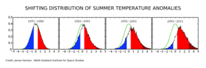
Frequency of occurrence (vertical axis) of local June–July–August temperature anomalies (relative to 1951–1980 mean) for Northern Hemisphere land in units of local standard deviation (horizontal axis). According to Hansen et al. (2012), the distribution of anomalies has shifted to the right as a consequence of global warming, meaning that unusually hot summers have become more common. This is analogous to the rolling of a dice: cool summers now cover only half of one side of a six-sided die, white covers one side, red covers four sides, and an extremely hot (red-brown) anomaly covers half of one side.

One of the subjects discussed in the literature is whether or not extreme weather events can be attributed to human activities. Seneviratne et al. (2012) stated that attributing individual extreme weather events to human activities was challenging. They were, however, more confident over attributing changes in long-term trends of extreme weather. For example, Seneviratne et al. (2012) concluded that human activities had likely led to a warming of extreme daily minimum and maximum temperatures at the global scale.

Another way of viewing the problem is to consider the effects of human-induced climate change on the probability of future extreme weather events. Stott et al. (2003), for example, considered whether or not human activities had increased the risk of severe heat waves in Europe, like the one experienced in 2003. Their conclusion was that human activities had very likely more than doubled the risk of heat waves of this magnitude.

An analogy can be made between an athlete on steroids and human-induced climate change. In the same way that an athlete's performance may increase from using steroids, human-induced climate change increases the risk of some extreme weather events.

Hansen et al. (2012) suggested that human activities have greatly increased the risk of summertime heat waves. According to their analysis, the land area of the Earth affected by very hot summer temperature anomalies has greatly increased over time (refer to graphs on the left). In the base period 1951–1980, these anomalies covered a few tenths of 1% of the global land area. In recent years, this has increased to around 10% of the global land area. With high confidence, Hansen et al. (2012) attributed the 2010 Moscow and 2011 Texas heat waves to human-induced global warming.

An earlier study by Dole et al. (2011) concluded that the 2010 Moscow heatwave was mostly due to natural weather variability. While not directly citing Dole et al. (2011), Hansen et al. (2012) rejected this type of explanation. Hansen et al. (2012) stated that a combination of natural weather variability and human-induced global warming was responsible for the Moscow and Texas heat waves.

Scientific literature and opinion

There are a number of examples of published and informal support for the consensus view. As mentioned earlier, the IPCC has concluded that most of the observed increase in globally averaged temperatures since the mid-20th century is "very likely" due to human activities. The IPCC's conclusions are consistent with those of several reports produced by the US National Research Council. A report published in 2009 by the U.S. Global Change Research Program concluded that "[global] warming is unequivocal and primarily human-induced." A number of scientific organizations have issued statements that support the consensus view. Two examples include:

Detection and attribution studies

Refer to caption
This image shows three examples of internal climate variability measured between 1950 and 2012: the El Niño–Southern oscillation, the Arctic oscillation, and the North Atlantic oscillation.

The IPCC Fourth Assessment Report (2007), concluded that attribution was possible for a number of observed changes in the climate (see effects of global warming). However, attribution was found to be more difficult when assessing changes over smaller regions (less than continental scale) and over short time periods (less than 50 years). Over larger regions, averaging reduces natural variability of the climate, making detection and attribution easier.

  • In 1996, in a paper in Nature titled "A search for human influences on the thermal structure of the atmosphere", Benjamin D. Santer et al. wrote: "The observed spatial patterns of temperature change in the free atmosphere from 1963 to 1987 are similar to those predicted by state-of-the-art climate models incorporating various combinations of changes in carbon dioxide, anthropogenic sulphate aerosol and stratospheric ozone concentrations. The degree of pattern similarity between models and observations increases through this period. It is likely that this trend is partially due to human activities, although many uncertainties remain, particularly relating to estimates of natural variability."
  • A 2002 paper in the Journal of Geophysical Research says "Our analysis suggests that the early twentieth century warming can best be explained by a combination of warming due to increases in greenhouse gases and natural forcing, some cooling due to other anthropogenic forcings, and a substantial, but not implausible, contribution from internal variability. In the second half of the century we find that the warming is largely caused by changes in greenhouse gases, with changes in sulphates and, perhaps, volcanic aerosol offsetting approximately one third of the warming."
  • A 2005 review of detection and attribution studies by the International Ad hoc Detection and Attribution Group found that "natural drivers such as solar variability and volcanic activity are at most partially responsible for the large-scale temperature changes observed over the past century, and that a large fraction of the warming over the last 50 yr can be attributed to greenhouse gas increases. Thus, the recent research supports and strengthens the IPCC Third Assessment Report conclusion that 'most of the global warming over the past 50 years is likely due to the increase in greenhouse gases.'"
  • Barnett and colleagues (2005) say that the observed warming of the oceans "cannot be explained by natural internal climate variability or solar and volcanic forcing, but is well simulated by two anthropogenically forced climate models," concluding that "it is of human origin, a conclusion robust to observational sampling and model differences".
  • Two papers in the journal Science in August 2005 resolve the problem, evident at the time of the TAR, of tropospheric temperature trends (see also the section on "fingerprint" studies) . The UAH version of the record contained errors, and there is evidence of spurious cooling trends in the radiosonde record, particularly in the tropics. See satellite temperature measurements for details; and the 2006 US CCSP report.
  • Multiple independent reconstructions of the temperature record of the past 1000 years confirm that the late 20th century is probably the warmest period in that time (see the preceding section -details on attribution).

Reviews of scientific opinion

  • An essay in Science surveyed 928 abstracts related to climate change, and concluded that most journal reports accepted the consensus. This is discussed further in scientific consensus on climate change.
  • A 2010 paper in the Proceedings of the National Academy of Sciences found that among a pool of roughly 1,000 researchers who work directly on climate issues and publish the most frequently on the subject, 97% agree that anthropogenic climate change is happening.
  • A 2011 paper from George Mason University published in the International Journal of Public Opinion Research, "The Structure of Scientific Opinion on Climate Change," collected the opinions of scientists in the earth, space, atmospheric, oceanic or hydrological sciences. The 489 survey respondents—representing nearly half of all those eligible according to the survey's specific standards – work in academia, government, and industry, and are members of prominent professional organizations. The study found that 97% of the 489 scientists surveyed agreed that global temperatures have risen over the past century. Moreover, 84% agreed that "human-induced greenhouse warming" is now occurring." Only 5% disagreed with the idea that human activity is a significant cause of global warming.

As described above, a small minority of scientists do disagree with the consensus. For example, Willie Soon and Richard Lindzen say that there is insufficient proof for anthropogenic attribution. Generally this position requires new physical mechanisms to explain the observed warming.

Solar activity

The graph shows the solar irradiance without a long-term trend. The 11-year solar cycle is also visible. The temperature, in contrast, shows an upward trend.
Solar irradiance (yellow) plotted together with temperature (red) over 1880 to 2018.
 
Modeled simulation of the effect of various factors (including GHGs, Solar irradiance) singly and in combination, showing in particular that solar activity produces a small and nearly uniform warming, unlike what is observed.

Solar sunspot maximum occurs when the magnetic field of the Sun collapses and reverse as part of its average 11-year solar cycle (22 years for complete North to North restoration).

The role of the Sun in recent climate change has been looked at by climate scientists. Since 1978, output from the Sun has been measured by satellites significantly more accurately than was previously possible from the surface. These measurements indicate that the Sun's total solar irradiance has not increased since 1978, so the warming during the past 30 years cannot be directly attributed to an increase in total solar energy reaching the Earth (see graph above, left). In the three decades since 1978, the combination of solar and volcanic activity probably had a slight cooling influence on the climate.

Climate models have been used to examine the role of the Sun in recent climate change. Models are unable to reproduce the rapid warming observed in recent decades when they only take into account variations in total solar irradiance and volcanic activity. Models are, however, able to simulate the observed 20th century changes in temperature when they include all of the most important external forcings, including human influences and natural forcings. As has already been stated, Hegerl et al. (2007) concluded that greenhouse gas forcing had "very likely" caused most of the observed global warming since the mid-20th century. In making this conclusion, Hegerl et al. (2007) allowed for the possibility that climate models had been underestimated the effect of solar forcing.

The role of solar activity in climate change has also been calculated over longer time periods using "proxy" datasets, such as tree rings. Models indicate that solar and volcanic forcings can explain periods of relative warmth and cold between AD 1000 and 1900, but human-induced forcings are needed to reproduce the late-20th century warming.

Another line of evidence against the sun having caused recent climate change comes from looking at how temperatures at different levels in the Earth's atmosphere have changed. Models and observations (see figure above, middle) show that greenhouse gas results in warming of the lower atmosphere at the surface (called the troposphere) but cooling of the upper atmosphere (called the stratosphere). Depletion of the ozone layer by chemical refrigerants has also resulted in a cooling effect in the stratosphere. If the Sun was responsible for observed warming, warming of the troposphere at the surface and warming at the top of the stratosphere would be expected as increase solar activity would replenish ozone and oxides of nitrogen. The stratosphere has a reverse temperature gradient than the troposphere so as the temperature of the troposphere cools with altitude, the stratosphere rises with altitude. Hadley cells are the mechanism by which equatorial generated ozone in the tropics (highest area of UV irradiance in the stratosphere) is moved poleward. Global climate models suggest that climate change may widen the Hadley cells and push the jetstream northward thereby expanding the tropics region and resulting in warmer, dryer conditions in those areas overall.

Non-consensus views

Habibullo Abdussamatov (2004), head of space research at St. Petersburg's Pulkovo Astronomical Observatory in Russia, has argued that the sun is responsible for recently observed climate change. Journalists for news sources canada.com (Solomon, 2007b), National Geographic News (Ravilious, 2007), and LiveScience (Than, 2007) reported on the story of warming on Mars. In these articles, Abdussamatov was quoted. He stated that warming on Mars was evidence that global warming on Earth was being caused by changes in the sun.

Ravilious (2007) quoted two scientists who disagreed with Abdussamatov: Amato Evan, a climate scientist at the University of Wisconsin–Madison, in the US, and Colin Wilson, a planetary physicist at Oxford University in the UK. According to Wilson, "Wobbles in the orbit of Mars are the main cause of its climate change in the current era" (see also orbital forcing). Than (2007) quoted Charles Long, a climate physicist at Pacific Northwest National Laboratories in the US, who disagreed with Abdussamatov.

Than (2007) pointed to the view of Benny Peiser, a social anthropologist at Liverpool John Moores University in the UK. In his newsletter, Peiser had cited a blog that had commented on warming observed on several planetary bodies in the Solar system. These included Neptune's moon Triton, Jupiter, Pluto and Mars. In an e-mail interview with Than (2007), Peiser stated that:

"I think it is an intriguing coincidence that warming trends have been observed on a number of very diverse planetary bodies in our solar system, (...) Perhaps this is just a fluke."

Than (2007) provided alternative explanations of why warming had occurred on Triton, Pluto, Jupiter and Mars.

The US Environmental Protection Agency (US EPA, 2009) responded to public comments on climate change attribution. A number of commenters had argued that recent climate change could be attributed to changes in solar irradiance. According to the US EPA (2009), this attribution was not supported by the bulk of the scientific literature. Citing the work of the IPCC (2007), the US EPA pointed to the low contribution of solar irradiance to radiative forcing since the start of the Industrial Revolution in 1750. Over this time period (1750 to 2005), the estimated contribution of solar irradiance to radiative forcing was 5% the value of the combined radiative forcing due to increases in the atmospheric concentrations of carbon dioxide, methane and nitrous oxide (see graph opposite).

Effect of cosmic rays

Henrik Svensmark has suggested that the magnetic activity of the sun deflects cosmic rays, and that this may influence the generation of cloud condensation nuclei, and thereby have an effect on the climate. The website ScienceDaily reported on a 2009 study that looked at how past changes in climate have been affected by the Earth's magnetic field. Geophysicist Mads Faurschou Knudsen, who co-authored the study, stated that the study's results supported Svensmark's theory. The authors of the study also acknowledged that CO
2
plays an important role in climate change.

Consensus view on cosmic rays

The view that cosmic rays could provide the mechanism by which changes in solar activity affect climate is not supported by the literature. Solomon et al. (2007) state:

[..] the cosmic ray time series does not appear to correspond to global total cloud cover after 1991 or to global low-level cloud cover after 1994. Together with the lack of a proven physical mechanism and the plausibility of other causal factors affecting changes in cloud cover, this makes the association between galactic cosmic ray-induced changes in aerosol and cloud formation controversial

Studies by Lockwood and Fröhlich (2007) and Sloan and Wolfendale (2008) found no relation between warming in recent decades and cosmic rays. Pierce and Adams (2009) used a model to simulate the effect of cosmic rays on cloud properties. They concluded that the hypothesized effect of cosmic rays was too small to explain recent climate change. Pierce and Adams (2009) noted that their findings did not rule out a possible connection between cosmic rays and climate change, and recommended further research.

Erlykin et al. (2009) found that the evidence showed that connections between solar variation and climate were more likely to be mediated by direct variation of insolation rather than cosmic rays, and concluded: "Hence within our assumptions, the effect of varying solar activity, either by direct solar irradiance or by varying cosmic ray rates, must be less than 0.07 °C since 1956, i.e. less than 14% of the observed global warming." Carslaw (2009) and Pittock (2009) review the recent and historical literature in this field and continue to find that the link between cosmic rays and climate is tenuous, though they encourage continued research. US EPA (2009) commented on research by Duplissy et al. (2009):

The CLOUD experiments at CERN are interesting research but do not provide conclusive evidence that cosmic rays can serve as a major source of cloud seeding. Preliminary results from the experiment (Duplissy et al., 2009) suggest that though there was some evidence of ion mediated nucleation, for most of the nucleation events observed the contribution of ion processes appeared to be minor. These experiments also showed the difficulty in maintaining sufficiently clean conditions and stable temperatures to prevent spurious aerosol bursts. There is no indication that the earlier Svensmark experiments could even have matched the controlled conditions of the CERN experiment. We find that the Svensmark results on cloud seeding have not yet been shown to be robust or sufficient to materially alter the conclusions of the assessment literature, especially given the abundance of recent literature that is skeptical of the cosmic ray-climate linkage.
Saturday, November 21, 2020

Earth Simulator

From Wikipedia, the free encyclopedia
 
Earth Simulator (ES), original version
 
Earth Simulator interconnection rack
 
Earth Simulator processing rack
 
Earth Simulator arithmetic processing module
 
Earth Simulator 2 (ES2)
Earth Simulator 3 (ES3)

The Earth Simulator (ES) (地球シミュレータ, Chikyū Shimyurēta), developed by the Japanese government's initiative "Earth Simulator Project", was a highly parallel vector supercomputer system for running global climate models to evaluate the effects of global warming and problems in solid earth geophysics. The system was developed for Japan Aerospace Exploration Agency, Japan Atomic Energy Research Institute, and Japan Marine Science and Technology Center (JAMSTEC) in 1997.

Construction started in October 1999, and the site officially opened on 11 March 2002. The project cost 60 billion yen.

Built by NEC, ES was based on their SX-6 architecture. It consisted of 640 nodes with eight vector processors and 16 gigabytes of computer memory at each node, for a total of 5120 processors and 10 terabytes of memory. Two nodes were installed per 1 metre × 1.4 metre × 2 metre cabinet. Each cabinet consumed 20 kW of power. The system had 700 terabytes of disk storage (450 for the system and 250 for the users) and 1.6 petabytes of mass storage in tape drives. It was able to run holistic simulations of global climate in both the atmosphere and the oceans down to a resolution of 10 km. Its performance on the LINPACK benchmark was 35.86 TFLOPS, which was almost five times faster than the previous fastest supercomputer, ASCI White. As of 2020, comparable performance can be achieved by using 4 Nvidia A100 GPUs, each with 9.746 FP64 TFlops.

ES was the fastest supercomputer in the world from 2002 to 2004. Its capacity was surpassed by IBM's Blue Gene/L prototype on 29 September 2004.

ES was replaced by the Earth Simulator 2 (ES2) in March 2009. ES2 is an NEC SX-9/E system, and has a quarter as many nodes each of 12.8 times the performance (3.2× clock speed, four times the processing resource per node), for a peak performance of 131 TFLOPS. With a delivered LINPACK performance of 122.4 TFLOPS, ES2 was the most efficient supercomputer in the world at that point. In November 2010, NEC announced that ES2 topped the Global FFT, one of the measures of the HPC Challenge Awards, with the performance number of 11.876 TFLOPS.

ES2 was replaced by the Earth Simulator 3 (ES3) in March 2015. ES3 is a NEC SX-ACE system with 5120 nodes, and a performance of 1.3 PFLOPS.

ES3, from 2017 to 2018, ran alongside Gyoukou, a supercomputer with immersion cooling that can achieve up to 19 PFLOPS.

System overview

Hardware

The Earth Simulator (ES for short) was developed as a national project by three governmental agencies: the National Space Development Agency of Japan (NASDA), the Japan Atomic Energy Research Institute (JAERI), and the Japan Marine Science and Technology Center (JAMSTEC). The ES is housed in the Earth Simulator Building (approx; 50m × 65m × 17m). The Earth Simulator 2 (ES2) uses 160 nodes of NEC's SX-9E. The upgrade of the Earth Simulator has been completed in March 2015. The Earth Simulator 3(ES3) system uses 5120 nodes of NEC's SX-ACE.

System configuration

The ES is a highly parallel vector supercomputer system of the distributed-memory type, and consisted of 160 processor nodes connected by Fat-Tree Network. Each Processor nodes is a system with a shared memory, consisting of 8 vector-type arithmetic processors, a 128-GB main memory system. The peak performance of each Arithmetic processors is 102.4Gflops. The ES as a whole thus consists of 1280 arithmetic processors with 20 TB of main memory and the theoretical performance of 131Tflops.

Construction of CPU

Each CPU consists of a 4-way super-scalar unit (SU), a vector unit (VU), and main memory access control unit on a single LSI chip. The CPU operates at a clock frequency of 3.2 GHz. Each VU has 72 vector registers, each of which has 256 vector elements, along with 8 sets of six different types of vector pipelines: addition /shifting, multiplication, division, logical operations, masking, and load/store. The same type of vector pipelines works together by a single vector instruction and pipelines of different types can operate concurrently.

Processor Node (PN)

The processor node is composed of 8 CPU and 10 memory modules.

Interconnection Network (IN)

The RCU is directly connected to the crossbar switches and controls inter-node data communications at 64 GB/s bidirectional transfer rate for both sending and receiving data. Thus the total bandwidth of inter-node network is about 10 TB/s.

Processor Node (PN) Cabinet

The processor node is composed two nodes of one cabinet, and consists of power supply part 8 memory modules and PCI box with 8 CPU modules.

Software

Below is the description of software technologies used in the operating system, Job Scheduling and the programming environment of ES2.

Operating system

The operating system running on ES, "Earth Simulator Operating System", is a custom version of NEC's SUPER-UX used for the NEC SX supercomputers that make up ES.

Mass storage file system

If a large parallel job running on 640 PNs reads from/writes to one disk installed in a PN, each PN accesses to the disk in sequence and performance degrades terribly. Although local I/O in which each PN reads from or writes to its own disk solves the problem, it is a very hard work to manage such a large number of partial files. Then ES adopts Staging and Global File System (GFS) that offers a high-speed I/O performance.

Job scheduling

ES is basically a batch-job system. Network Queuing System II (NQSII) is introduced to manage the batch job. Queue configuration of the Earth Simulator. ES has two-type queues. S batch queue is designed for single-node batch jobs and L batch queue is for multi-node batch queue. There are two-type queues. One is L batch queue and the other is S batch queue. S batch queue is aimed at being used for a pre-run or a post-run for large-scale batch jobs (making initial data, processing results of a simulation and other processes), and L batch queue is for a production run. Users choose the appropriate queue for their job.

  1. The nodes allocated to a batch job are used exclusively for that batch job.
  2. The batch job is scheduled based on elapsed time instead of CPU time.

Strategy (1) enables to estimate the job termination time and to make it easy to allocate nodes for the next batch jobs in advance. Strategy (2) contributes to an efficient job execution. The job can use the nodes exclusively and the processes in each node can be executed simultaneously. As a result, the large-scale parallel program is able to be executed efficiently. PNs of L-system are prohibited from access to the user disk to ensure enough disk I/O performance. herefore the files used by the batch job are copied from the user disk to the work disk before the job execution. This process is called "stage-in." It is important to hide this staging time for the job scheduling. Main steps of the job scheduling are summarized as follows;

  1. Node Allocation
  2. Stage-in (copies files from the user disk to the work disk automatically)
  3. Job Escalation (rescheduling for the earlier estimated start time if possible)
  4. Job Execution
  5. Stage-out (copies files from the work disk to the user disk automatically)

When a new batch job is submitted, the scheduler searches available nodes (Step.1). After the nodes and the estimated start time are allocated to the batch job, stage-in process starts (Step.2). The job waits until the estimated start time after stage-in process is finished. If the scheduler find the earlier start time than the estimated start time, it allocates the new start time to the batch job. This process is called "Job Escalation" (Step.3). When the estimated start time has arrived, the scheduler executes the batch job (Step.4). The scheduler terminates the batch job and starts stage-out process after the job execution is finished or the declared elapsed time is over (Step.5). To execute the batch job, the user logs into the login-server and submits the batch script to ES. And the user waits until the job execution is done. During that time, the user can see the state of the batch job using the conventional web browser or user commands. The node scheduling, the file staging and other processing are automatically processed by the system according to the batch script.

Programming environment

Programming model in ES

The ES hardware has a 3-level hierarchy of parallelism: vector processing in an AP, parallel processing with shared memory in a PN, and parallel processing among PNs via IN. To bring out high performance of ES fully, you must develop parallel programs that make the most use of such parallelism. the 3-level hierarchy of parallelism of ES can be used in two manners, which are called hybrid and flat parallelization, respectively . In the hybrid parallelization, the inter-node parallelism is expressed by HPF or MPI, and the intra-node by microtasking or OpenMP, and you must, therefore, consider the hierarchical parallelism in writing your programs. In the flat parallelization, the both inter- and intra-node parallelism can be expressed by HPF or MPI, and it is not necessary for you to consider such complicated parallelism. Generally speaking, the hybrid parallelization is superior to the flat in performance and vice versa in ease of programming. Note that the MPI libraries and the HPF runtimes are optimized to perform as well as possible both in the hybrid and flat parallelization.

Languages

Compilers for Fortran 90, C and C++ are available. All of them have an advanced capability of automatic vectorization and microtasking. Microtasking is a sort of multitasking provided for the Cray's supercomputer at the same time and is also used for intra-node parallelization on ES. Microtasking can be controlled by inserting directives into source programs or using the compiler's automatic parallelization. (Note that OpenMP is also available in Fortran 90 and C++ for intra-node parallelization.)

Parallelization

Message Passing Interface (MPI)

MPI is a message passing library based on the MPI-1 and MPI-2 standards and provides high-speed communication capability that fully exploits the features of IXS and shared memory. It can be used for both intra- and inter-node parallelization. An MPI process is assigned to an AP in the flat parallelization, or to a PN that contains microtasks or OpenMP threads in the hybrid parallelization. MPI libraries are designed and optimizedcarefully to achieve highest performance of communication on the ES architecture in both of the parallelization manner.

High Performance Fortrans (HPF)

Principal users of ES are considered to be natural scientists who are not necessarily familiar with the parallel programming or rather dislike it. Accordingly, a higher-level parallel language is in great demand. HPF/SX provides easy and efficient parallel programming on ES to supply the demand. It supports the specifications of HPF2.0, its approved extensions, HPF/JA, and some unique extensions for ES

Tools

-Integrated development environment (PSUITE)

Integrated development environment (PSUITE) is integration of various tools to develop the program that operates by SUPER-UX. Because PSUITE assumes that various tools can be used by GUI, and has the coordinated function between tools, it comes to be able to develop the program more efficiently than the method of developing the past the program and easily.

-Debug Support

In SUPER-UX, the following are prepared as strong debug support functions to support the program development.

Facilities

Features of the Earth Simulator building

Protection from natural disasters

The Earth Simulator Center has several special features that help to protect the computer from natural disasters or occurrences. A wire nest hangs over the building which helps to protect from lightning. The nest itself uses high-voltage shielded cables to release lightning current into the ground. A special light propagation system utilizes halogen lamps, installed outside of the shielded machine room walls, to prevent any magnetic interference from reaching the computers. The building is constructed on a seismic isolation system, composed of rubber supports, that protect the building during earthquakes.

Lightning protection system

Three basic features:

  • Four poles at both sides of the Earth Simulator Building compose wire nest to protect the building from lightning strikes.
  • Special high-voltage shielded cable is used for inductive wire which releases a lightning current to the earth.
  • Ground plates are laid by keeping apart from the building about 10 meters.

Illumination

Lighting: Light propagation system inside a tube (255mm diameter, 44m(49yd) length, 19 tubes) Light source: halogen lamps of 1 kW Illumination: 300 lx at the floor in average The light sources installed out of the shielded machine room walls.

Seismic isolation system

11 isolators (1 ft height, 3.3 ft. Diameter, 20-layered rubbers supporting the bottom of the ES building)

Performance

LINPACK

The new Earth Simulator system, which began operation in March 2009, achieved sustained performance of 122.4 TFLOPS and computing efficiency (*2) of 93.38% on the LINPACK Benchmark (*1).

  • 1. LINPACK Benchmark

The LINPACK Benchmark is a measure of a computer's performance and is used as a standard benchmark to rank computer systems in the TOP500 project. LINPACK is a program for performing numerical linear algebra on computers.

  • 2. Computing efficiency

Computing efficiency is the ratio of sustained performance to a peak computing performance. Here, it is the ratio of 122.4TFLOPS to 131.072TFLOPS.

Computational performance of WRF on Earth Simulator

WRF (Weather Research and Forecasting Model) is a mesoscale meteorological simulation code which has been developed under the collaboration among US institutions, including NCAR (National Center for Atmospheric Research) and NCEP (National Centers for Environmental Prediction). JAMSTEC has optimized WRFV2 on the Earth Simulator (ES2) renewed in 2009 with the measurement of computational performance. As a result, it was successfully demonstrated that WRFV2 can run on the ES2 with outstanding and sustained performance.

The numerical meteorological simulation was conducted by using WRF on the Earth Simulator for the earth's hemisphere with the Nature Run model condition. The model spatial resolution is 4486 by 4486 horizontally with the grid spacing of 5 km and 101 levels vertically. Mostly adiabatic conditions were applied with the time integration step of 6 seconds. A very high performance on the Earth Simulator was achieved for high-resolution WRF. While the number of CPU cores used is only 1% as compared to the world fastest class system Jaguar (CRAY XT5) at Oak Ridge National Laboratory, the sustained performance obtained on the Earth Simulator is almost 50% of that measured on the Jaguar system. The peak performance ratio on the Earth Simulator is also record-high 22.2%.

General circulation model

From Wikipedia, the free encyclopedia

Climate models are systems of differential equations based on the basic laws of physics, fluid motion, and chemistry. To "run" a model, scientists divide the planet into a 3-dimensional grid, apply the basic equations, and evaluate the results. Atmospheric models calculate winds, heat transfer, radiation, relative humidity, and surface hydrology within each grid and evaluate interactions with neighboring points.
 
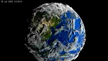
This visualization shows early test renderings of a global computational model of Earth's atmosphere based on data from NASA's Goddard Earth Observing System Model, Version 5 (GEOS-5).

A general circulation model (GCM) is a type of climate model. It employs a mathematical model of the general circulation of a planetary atmosphere or ocean. It uses the Navier–Stokes equations on a rotating sphere with thermodynamic terms for various energy sources (radiation, latent heat). These equations are the basis for computer programs used to simulate the Earth's atmosphere or oceans. Atmospheric and oceanic GCMs (AGCM and OGCM) are key components along with sea ice and land-surface components.

GCMs and global climate models are used for weather forecasting, understanding the climate, and forecasting climate change.

Versions designed for decade to century time scale climate applications were originally created by Syukuro Manabe and Kirk Bryan at the Geophysical Fluid Dynamics Laboratory (GFDL) in Princeton, New Jersey. These models are based on the integration of a variety of fluid dynamical, chemical and sometimes biological equations.

Terminology

The acronym GCM originally stood for General Circulation Model. Recently, a second meaning came into use, namely Global Climate Model. While these do not refer to the same thing, General Circulation Models are typically the tools used for modelling climate, and hence the two terms are sometimes used interchangeably. However, the term "global climate model" is ambiguous and may refer to an integrated framework that incorporates multiple components including a general circulation model, or may refer to the general class of climate models that use a variety of means to represent the climate mathematically.

History

In 1956, Norman Phillips developed a mathematical model that could realistically depict monthly and seasonal patterns in the troposphere. It became the first successful climate model. Following Phillips's work, several groups began working to create GCMs. The first to combine both oceanic and atmospheric processes was developed in the late 1960s at the NOAA Geophysical Fluid Dynamics Laboratory. By the early 1980s, the United States' National Center for Atmospheric Research had developed the Community Atmosphere Model; this model has been continuously refined. In 1996, efforts began to model soil and vegetation types. Later the Hadley Centre for Climate Prediction and Research's HadCM3 model coupled ocean-atmosphere elements. The role of gravity waves was added in the mid-1980s. Gravity waves are required to simulate regional and global scale circulations accurately.

Atmospheric and oceanic models

Atmospheric (AGCMs) and oceanic GCMs (OGCMs) can be coupled to form an atmosphere-ocean coupled general circulation model (CGCM or AOGCM). With the addition of submodels such as a sea ice model or a model for evapotranspiration over land, AOGCMs become the basis for a full climate model.

Structure

Three-dimensional (more properly four-dimensional) GCMs apply discrete equations for fluid motion and integrate these forward in time. They contain parameterisations for processes such as convection that occur on scales too small to be resolved directly.

A simple general circulation model (SGCM) consists of a dynamic core that relates properties such as temperature to others such as pressure and velocity. Examples are programs that solve the primitive equations, given energy input and energy dissipation in the form of scale-dependent friction, so that atmospheric waves with the highest wavenumbers are most attenuated. Such models may be used to study atmospheric processes, but are not suitable for climate projections.

Atmospheric GCMs (AGCMs) model the atmosphere (and typically contain a land-surface model as well) using imposed sea surface temperatures (SSTs). They may include atmospheric chemistry.

AGCMs consist of a dynamical core which integrates the equations of fluid motion, typically for:

  • surface pressure
  • horizontal components of velocity in layers
  • temperature and water vapor in layers
  • radiation, split into solar/short wave and terrestrial/infrared/long wave
  • parameters for:

A GCM contains prognostic equations that are a function of time (typically winds, temperature, moisture, and surface pressure) together with diagnostic equations that are evaluated from them for a specific time period. As an example, pressure at any height can be diagnosed by applying the hydrostatic equation to the predicted surface pressure and the predicted values of temperature between the surface and the height of interest. Pressure is used to compute the pressure gradient force in the time-dependent equation for the winds.

OGCMs model the ocean (with fluxes from the atmosphere imposed) and may contain a sea ice model. For example, the standard resolution of HadOM3 is 1.25 degrees in latitude and longitude, with 20 vertical levels, leading to approximately 1,500,000 variables.

AOGCMs (e.g. HadCM3, GFDL CM2.X) combine the two submodels. They remove the need to specify fluxes across the interface of the ocean surface. These models are the basis for model predictions of future climate, such as are discussed by the IPCC. AOGCMs internalise as many processes as possible. They have been used to provide predictions at a regional scale. While the simpler models are generally susceptible to analysis and their results are easier to understand, AOGCMs may be nearly as hard to analyse as the climate itself.

Grid

The fluid equations for AGCMs are made discrete using either the finite difference method or the spectral method. For finite differences, a grid is imposed on the atmosphere. The simplest grid uses constant angular grid spacing (i.e., a latitude / longitude grid). However, non-rectangular grids (e.g., icosahedral) and grids of variable resolution are more often used. The LMDz model can be arranged to give high resolution over any given section of the planet. HadGEM1 (and other ocean models) use an ocean grid with higher resolution in the tropics to help resolve processes believed to be important for the El Niño Southern Oscillation (ENSO). Spectral models generally use a gaussian grid, because of the mathematics of transformation between spectral and grid-point space. Typical AGCM resolutions are between 1 and 5 degrees in latitude or longitude: HadCM3, for example, uses 3.75 in longitude and 2.5 degrees in latitude, giving a grid of 96 by 73 points (96 x 72 for some variables); and has 19 vertical levels. This results in approximately 500,000 "basic" variables, since each grid point has four variables (u,v, T, Q), though a full count would give more (clouds; soil levels). HadGEM1 uses a grid of 1.875 degrees in longitude and 1.25 in latitude in the atmosphere; HiGEM, a high-resolution variant, uses 1.25 x 0.83 degrees respectively. These resolutions are lower than is typically used for weather forecasting. Ocean resolutions tend to be higher, for example HadCM3 has 6 ocean grid points per atmospheric grid point in the horizontal.

For a standard finite difference model, uniform gridlines converge towards the poles. This would lead to computational instabilities (see CFL condition) and so the model variables must be filtered along lines of latitude close to the poles. Ocean models suffer from this problem too, unless a rotated grid is used in which the North Pole is shifted onto a nearby landmass. Spectral models do not suffer from this problem. Some experiments use geodesic grids and icosahedral grids, which (being more uniform) do not have pole-problems. Another approach to solving the grid spacing problem is to deform a Cartesian cube such that it covers the surface of a sphere.

Flux buffering

Some early versions of AOGCMs required an ad hoc process of "flux correction" to achieve a stable climate. This resulted from separately prepared ocean and atmospheric models that each used an implicit flux from the other component different than that component could produce. Such a model failed to match observations. However, if the fluxes were 'corrected', the factors that led to these unrealistic fluxes might be unrecognised, which could affect model sensitivity. As a result, the vast majority of models used in the current round of IPCC reports do not use them. The model improvements that now make flux corrections unnecessary include improved ocean physics, improved resolution in both atmosphere and ocean, and more physically consistent coupling between atmosphere and ocean submodels. Improved models now maintain stable, multi-century simulations of surface climate that are considered to be of sufficient quality to allow their use for climate projections.

Convection

Moist convection releases latent heat and is important to the Earth's energy budget. Convection occurs on too small a scale to be resolved by climate models, and hence it must be handled via parameters. This has been done since the 1950s. Akio Arakawa did much of the early work, and variants of his scheme are still used, although a variety of different schemes are now in use. Clouds are also typically handled with a parameter, for a similar lack of scale. Limited understanding of clouds has limited the success of this strategy, but not due to some inherent shortcoming of the method.

Software

Most models include software to diagnose a wide range of variables for comparison with observations or study of atmospheric processes. An example is the 2-metre temperature, which is the standard height for near-surface observations of air temperature. This temperature is not directly predicted from the model but is deduced from surface and lowest-model-layer temperatures. Other software is used for creating plots and animations.

Projections

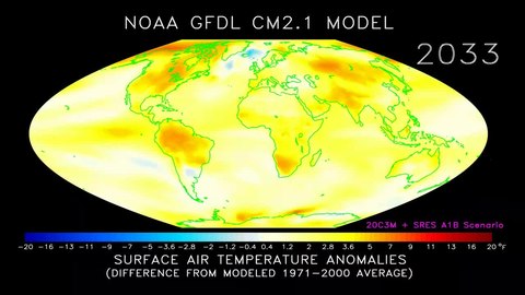
Projected annual mean surface air temperature from 1970-2100, based on SRES emissions scenario A1B, using the NOAA GFDL CM2.1 climate model (credit: NOAA Geophysical Fluid Dynamics Laboratory).

Coupled AOGCMs use transient climate simulations to project/predict climate changes under various scenarios. These can be idealised scenarios (most commonly, CO2 emissions increasing at 1%/yr) or based on recent history (usually the "IS92a" or more recently the SRES scenarios). Which scenarios are most realistic remains uncertain.

The 2001 IPCC Third Assessment Report F igure 9.3 shows the global mean response of 19 different coupled models to an idealised experiment in which emissions increased at 1% per year. Figure 9.5 shows the response of a smaller number of models to more recent trends. For the 7 climate models shown there, the temperature change to 2100 varies from 2 to 4.5 °C with a median of about 3 °C.

Future scenarios do not include unknown events – for example, volcanic eruptions or changes in solar forcing. These effects are believed to be small in comparison to greenhouse gas (GHG) forcing in the long term, but large volcanic eruptions, for example, can exert a substantial temporary cooling effect.

Human GHG emissions are a model input, although it is possible to include an economic/technological submodel to provide these as well. Atmospheric GHG levels are usually supplied as an input, though it is possible to include a carbon cycle model that reflects vegetation and oceanic processes to calculate such levels.

Emissions scenarios

In the 21st century, changes in global mean temperature are projected to vary across the world
Projected change in annual mean surface air temperature from the late 20th century to the middle 21st century, based on SRES emissions scenario A1B (credit: NOAA Geophysical Fluid Dynamics Laboratory).

For the six SRES marker scenarios, IPCC (2007:7–8) gave a "best estimate" of global mean temperature increase (2090–2099 relative to the period 1980–1999) of 1.8 °C to 4.0 °C. Over the same time period, the "likely" range (greater than 66% probability, based on expert judgement) for these scenarios was for a global mean temperature increase of 1.1 to 6.4 °C.

In 2008 a study made climate projections using several emission scenarios. In a scenario where global emissions start to decrease by 2010 and then declined at a sustained rate of 3% per year, the likely global average temperature increase was predicted to be 1.7 °C above pre-industrial levels by 2050, rising to around 2 °C by 2100. In a projection designed to simulate a future where no efforts are made to reduce global emissions, the likely rise in global average temperature was predicted to be 5.5 °C by 2100. A rise as high as 7 °C was thought possible, although less likely.

Another no-reduction scenario resulted in a median warming over land (2090–99 relative to the period 1980–99) of 5.1 °C. Under the same emissions scenario but with a different model, the predicted median warming was 4.1 °C.

Model accuracy

SST errors in HadCM3
 
North American precipitation from various models
 
Temperature predictions from some climate models assuming the SRES A2 emissions scenario

AOGCMs internalise as many processes as are sufficiently understood. However, they are still under development and significant uncertainties remain. They may be coupled to models of other processes in Earth system models, such as the carbon cycle, so as to better model feedbacks. Most recent simulations show "plausible" agreement with the measured temperature anomalies over the past 150 years, when driven by observed changes in greenhouse gases and aerosols. Agreement improves by including both natural and anthropogenic forcings.

Imperfect models may nevertheless produce useful results. GCMs are capable of reproducing the general features of the observed global temperature over the past century.

A debate over how to reconcile climate model predictions that upper air (tropospheric) warming should be greater than observed surface warming, some of which appeared to show otherwise, was resolved in favour of the models, following data revisions.

Cloud effects are a significant area of uncertainty in climate models. Clouds have competing effects on climate. They cool the surface by reflecting sunlight into space; they warm it by increasing the amount of infrared radiation transmitted from the atmosphere to the surface. In the 2001 IPCC report possible changes in cloud cover were highlighted as a major uncertainty in predicting climate.

Climate researchers around the world use climate models to understand the climate system. Thousands of papers have been published about model-based studies. Part of this research is to improve the models.

In 2000, a comparison between measurements and dozens of GCM simulations of ENSO-driven tropical precipitation, water vapor, temperature, and outgoing longwave radiation found similarity between measurements and simulation of most factors. However the simulated change in precipitation was about one-fourth less than what was observed. Errors in simulated precipitation imply errors in other processes, such as errors in the evaporation rate that provides moisture to create precipitation. The other possibility is that the satellite-based measurements are in error. Either indicates progress is required in order to monitor and predict such changes.

The precise magnitude of future changes in climate is still uncertain; for the end of the 21st century (2071 to 2100), for SRES scenario A2, the change of global average SAT change from AOGCMs compared with 1961 to 1990 is +3.0 °C (5.4 °F) and the range is +1.3 to +4.5 °C (+2.3 to 8.1 °F).

The IPCC's Fifth Assessment Report asserted "very high confidence that models reproduce the general features of the global-scale annual mean surface temperature increase over the historical period". However, the report also observed that the rate of warming over the period 1998–2012 was lower than that predicted by 111 out of 114 Coupled Model Intercomparison Project climate models.

Relation to weather forecasting

The global climate models used for climate projections are similar in structure to (and often share computer code with) numerical models for weather prediction, but are nonetheless logically distinct.

Most weather forecasting is done on the basis of interpreting numerical model results. Since forecasts are typically a few days or a week and sea surface temperatures change relatively slowly, such models do not usually contain an ocean model but rely on imposed SSTs. They also require accurate initial conditions to begin the forecast – typically these are taken from the output of a previous forecast, blended with observations. Weather predictions are required at higher temporal resolutions than climate projections, often sub-hourly compared to monthly or yearly averages for climate. However, because weather forecasts only cover around 10 days the models can also be run at higher vertical and horizontal resolutions than climate mode. Currently the ECMWF runs at 9 km (5.6 mi) resolution as opposed to the 100-to-200 km (62-to-124 mi) scale used by typical climate model runs. Often local models are run using global model results for boundary conditions, to achieve higher local resolution: for example, the Met Office runs a mesoscale model with an 11 km (6.8 mi) resolution covering the UK, and various agencies in the US employ models such as the NGM and NAM models. Like most global numerical weather prediction models such as the GFS, global climate models are often spectral models instead of grid models. Spectral models are often used for global models because some computations in modeling can be performed faster, thus reducing run times.

Computations

Climate models use quantitative methods to simulate the interactions of the atmosphere, oceans, land surface and ice.

All climate models take account of incoming energy as short wave electromagnetic radiation, chiefly visible and short-wave (near) infrared, as well as outgoing energy as long wave (far) infrared electromagnetic radiation from the earth. Any imbalance results in a change in temperature.

The most talked-about models of recent years relate temperature to emissions of greenhouse gases. These models project an upward trend in the surface temperature record, as well as a more rapid increase in temperature at higher altitudes.

Three (or more properly, four since time is also considered) dimensional GCM's discretise the equations for fluid motion and energy transfer and integrate these over time. They also contain parametrisations for processes such as convection that occur on scales too small to be resolved directly.

Atmospheric GCMs (AGCMs) model the atmosphere and impose sea surface temperatures as boundary conditions. Coupled atmosphere-ocean GCMs (AOGCMs, e.g. HadCM3, EdGCM, GFDL CM2.X, ARPEGE-Climat) combine the two models.

Models range in complexity:

  • A simple radiant heat transfer model treats the earth as a single point and averages outgoing energy
  • This can be expanded vertically (radiative-convective models), or horizontally
  • Finally, (coupled) atmosphere–ocean–sea ice global climate models discretise and solve the full equations for mass and energy transfer and radiant exchange.
  • Box models treat flows across and within ocean basins.

Other submodels can be interlinked, such as land use, allowing researchers to predict the interaction between climate and ecosystems.

Comparison with other climate models

Earth-system models of intermediate complexity (EMICs)

The Climber-3 model uses a 2.5-dimensional statistical-dynamical model with 7.5° × 22.5° resolution and time step of 1/2 a day. An oceanic submodel is MOM-3 (Modular Ocean Model) with a 3.75° × 3.75° grid and 24 vertical levels.

Radiative-convective models (RCM)

One-dimensional, radiative-convective models were used to verify basic climate assumptions in the 1980s and 1990s.

Earth system models

GCMs can form part of Earth system models, e.g. by coupling ice sheet models for the dynamics of the Greenland and Antarctic ice sheets, and one or more chemical transport models (CTMs) for species important to climate. Thus a carbon chemistry transport model may allow a GCM to better predict anthropogenic changes in carbon dioxide concentrations. In addition, this approach allows accounting for inter-system feedback: e.g. chemistry-climate models allow the effects of climate change on the ozone hole to be studied.

Climatology

From Wikipedia, the free encyclopedia

Climatology is the scientific study of the climate.

Climatology (from Greek κλίμα, klima, "place, zone"; and -λογία, -logia) or climate science is the scientific study of climate, scientifically defined as weather conditions averaged over a period of time. This modern field of study is regarded as a branch of the atmospheric sciences and a subfield of physical geography, which is one of the Earth sciences. Climatology now includes aspects of oceanography and biogeochemistry.

The main methods employed by climatologists are the analysis of observations and modelling the physical laws that determine the climate. The main topics of research are the study of climate variability, mechanisms of climate changes and modern climate change. Basic knowledge of climate can be used within shorter term weather forecasting, for instance about climatic cycles such as the El Niño–Southern Oscillation (ENSO), the Madden–Julian oscillation (MJO), the North Atlantic oscillation (NAO), the Arctic oscillation (AO), the Pacific decadal oscillation (PDO), and the Interdecadal Pacific Oscillation (IPO).

Climate models are used for a variety of purposes from study of the dynamics of the weather and climate system to projections of future climate. Weather is known as the condition of the atmosphere over a period of time, while climate has to do with the atmospheric condition over an extended to indefinite period of time.

History

The Greeks began the formal study of climate; in fact the word climate is derived from the Greek word klima, meaning "slope," referring to the slope or inclination of the Earth's axis. Arguably the most influential classic text on climate was On Airs, Water and Places written by Hippocrates around 400 BCE. This work commented on the effect of climate on human health and cultural differences between Asia and Europe. This idea that climate controls which countries excel depending on their climate, or climatic determinism, remained influential throughout history. Chinese scientist Shen Kuo (1031–1095) inferred that climates naturally shifted over an enormous span of time, after observing petrified bamboos found underground near Yanzhou (modern day Yan'an, Shaanxi province), a dry-climate area unsuitable for the growth of bamboo.

The invention of the thermometer and the barometer during the Scientific Revolution allowed for systematic recordkeeping, that began as early as 1640–1642 in England. Early climate researchers include Edmund Halley, who published a map of the trade winds in 1686 after a voyage to the southern hemisphere. Benjamin Franklin (1706–1790) first mapped the course of the Gulf Stream for use in sending mail from the United States to Europe. Francis Galton (1822–1911) invented the term anticyclone. Helmut Landsberg (1906–1985) fostered the use of statistical analysis in climatology, which led to its evolution into a physical science.

In the early 20th century, climatology was mostly focused on the description of regional climates. This descriptive climatology was mainly an applied science, giving farmers and other interested people statistics about what the normal weather was and how big chances were of extreme events. To do this, climatologists had to define a climate normal, or an average of weather and weather extremes over a period of typically 30 years.

Around the middle of the 20th century, many assumptions in meteorology and climatology considered climate to be roughly constant. While scientists knew of past climate change such as the ice ages, the concept of climate as unchanging was useful in the development of a general theory of what determines climate. This started to change in the decades that followed, and while the history of climate change science started earlier, climate change only became one of the mean topics of study for climatologists in the seventies and onward.

Subfields

Map of the average temperature over 30 years. Data sets formed from the long-term average of historical weather parameters are sometimes called a "climatology".

Various subfields of climatology study different aspects of the climate. There are different categorizations of the fields in climatology. The American Meteorological Society for instance identifies descriptive climatology, scientific climatology and applied climatology as the three subcategories of climatology, a categorization based on the complexity and the purpose of the research. Applied climatologists apply their expertise to different industries such as manufacturing and agriculture.

Paleoclimatology seeks to reconstruct and understand past climates by examining records such as ice cores and tree rings (dendroclimatology). Paleotempestology uses these same records to help determine hurricane frequency over millennia. Historical climatology is the study of climate as related to human history and thus focuses only on the last few thousand years.

Boundary-layer climatology is preoccupied with exchanges in water, energy and momentum near the surface. Further identified subfields are physical climatology, dynamic climatology, tornado climatology, regional climatology, bioclimatology, and synoptic climatology. The study of the hydrological cycle over long time scales (hydroclimatology) is further subdivided into the subfields of snow climatology and hail climatology.

Methods

The study of contemporary climates incorporates meteorological data accumulated over many years, such as records of rainfall, temperature and atmospheric composition. Knowledge of the atmosphere and its dynamics is also embodied in models, either statistical or mathematical, which help by integrating different observations and testing how they fit together. Modeling is used for understanding past, present and potential future climates.

Climate research is made difficult by the large scale, long time periods, and complex processes which govern climate. Climate is governed by physical laws which can be expressed as differential equations. These equations are coupled and nonlinear, so that approximate solutions are obtained by using numerical methods to create global climate models. Climate is sometimes modeled as a stochastic process but this is generally accepted as an approximation to processes that are otherwise too complicated to analyze.

Climate data

The collection of long record of climate variables is essential for the study of climate. Climatology deals with the aggregate data that meteorology has collected. Scientists use both direct and indirect observations of the climate, from Earth observing satellites and scientific instrumentation such as a global network of thermometers, to prehistoric ice extracted from glaciers. As measuring technology changes over time, records of data cannot be compared directly. As cities are generally warmer than the surrounding areas, urbanization has made it necessary to constantly correct data for this urban heat island effect.

Models

Climate models use quantitative methods to simulate the interactions of the atmosphere, oceans, land surface, and ice. They are used for a variety of purposes from study of the dynamics of the weather and climate system to projections of future climate. All climate models balance, or very nearly balance, incoming energy as short wave (including visible) electromagnetic radiation to the earth with outgoing energy as long wave (infrared) electromagnetic radiation from the earth. Any unbalance results in a change in the average temperature of the earth. Most climate models include the radiative effects of greenhouse gases such as carbon dioxide. These models predict an upward trend in the surface temperatures, as well as a more rapid increase in temperature at higher latitudes.

Models can range from relatively simple to complex:

  • A simple radiant heat transfer model that treats the earth as a single point and averages outgoing energy
  • this can be expanded vertically (radiative-convective models), or horizontally
  • Coupled atmosphere–ocean–sea ice global climate models discretise and solve the full equations for mass and energy transfer and radiant exchange.
  • Earth system models further include the biosphere.

Topics of research

Topics that climatologists study fall roughly into three categories: climate variability, mechanisms of climate change and modern climate change.

Climatological processes

Various factors impact the average state of the atmosphere at a particular location. For instance, midlatitudes will have a pronounced seasonal cycle in temperature whereas tropical regions show little variation in temperature over the year. Another major control in climate is continentality: the distance to major water bodies such as oceans. Oceans act as a moderating factor, so that land close to it has typically has mild winters and moderate summers. The atmosphere interacts with other spheres of the climate system, with winds generating ocean currents that transport heat around the globe.

Climate classification

Classification is an important aspect of many sciences as a tool of simplifying complicated processes. Different climate classifications have been developed over the centuries, with the first ones in Ancient Greece. How climates are classified depends on what the application is. A wind energy producer will require different information (wind) in the classification than somebody interested in agriculture, for who precipitation and temperature are more important. The most widely used classification, the Köppen climate classification, was developed in the late nineteenth century and is based on vegetation. It uses monthly temperature and precipitation data.

Climate variability

El Niño impacts

There are different modes of variability: recurring patterns of temperature or other climate variables. They are quantified with different indices. Much in the way the Dow Jones Industrial Average, which is based on the stock prices of 30 companies, is used to represent the fluctuations in the stock market as a whole, climate indices are used to represent the essential elements of climate. Climate indices are generally devised with the twin objectives of simplicity and completeness, and each index typically represents the status and timing of the climate factor it represents. By their very nature, indices are simple, and combine many details into a generalized, overall description of the atmosphere or ocean which can be used to characterize the factors which impact the global climate system.

El Niño–Southern Oscillation (ENSO) is a coupled ocean-atmosphere phenomenon in the Pacific Ocean responsible for most of the global variability in temperature, and has a cycle between two and seven years. The North Atlantic oscillation is a mode of variability that is mainly contained to the lower atmosphere, the troposphere. The layer of atmosphere above, the stratosphere is also capable of creating its own variability, most importantly in the Madden–Julian oscillation (MJO), which has a cycle of approximately 30-60 days. The interdecadal pacific oscillation can create changes in the Pacific Ocean and lower atmosphere on decadal time scales.

Climatic change

Climate change occurs when changes in Earth's climate system result in new weather patterns that remain in place for an extended period of time. This length of time can be as short as a few decades to as long as millions of years. The climate system receives nearly all of its energy from the sun. The climate system also gives off energy to outer space. The balance of incoming and outgoing energy, and the passage of the energy through the climate system, determines Earth's energy budget. When the incoming energy is greater than the outgoing energy, earth's energy budget is positive and the climate system is warming. If more energy goes out, the energy budget is negative and earth experiences cooling. Climate change also influences the average sea level.

Modern climate change is driven by the human emissions of greenhouse gas from the burning of fossil fuel driving up global mean surface temperatures. Rising temperatures are only one aspect of modern climate change though, with includes observed changes in precipitation, storm tracks and cloudiness. Warmer temperatures are driving further changes in the climate system, such as the widespread melt of glaciers, sea level rise and shifts in flora and fauna.

Differences with meteorology

In contrast to meteorology, which focuses on short term weather systems lasting up to a few weeks, climatology studies the frequency and trends of those systems. It studies the periodicity of weather events over years to millennia, as well as changes in long-term average weather patterns, in relation to atmospheric conditions. Climatologists study both the nature of climates – local, regional or global – and the natural or human-induced factors that cause climates to change. Climatology considers the past and can help predict future climate change.

Phenomena of climatological interest include the atmospheric boundary layer, circulation patterns, heat transfer (radiative, convective and latent), interactions between the atmosphere and the oceans and land surface (particularly vegetation, land use and topography), and the chemical and physical composition of the atmosphere.

Use in weather forecasting

A more complicated way of making a forecast, the analog technique requires remembering a previous weather event which is expected to be mimicked by an upcoming event. What makes it a difficult technique to use is that there is rarely a perfect analog for an event in the future. Some call this type of forecasting pattern recognition, which remains a useful method of observing rainfall over data voids such as oceans with knowledge of how satellite imagery relates to precipitation rates over land, as well as the forecasting of precipitation amounts and distribution in the future. A variation on this theme is used in medium range forecasting, which is known as teleconnections, when systems in other locations are used to help pin down the location of a system within the surrounding regime. One method of using teleconnections are by using climate indices such as ENSO-related phenomena.

Electronics

From Wikipedia, the free encyclopedia https://en.wikipedia.org/wiki/Electroni...