Quantum thermodynamics

From Wikipedia, the free encyclopedia

https://en.wikipedia.org/wiki/Quantum_thermodynamics 

 

Thermodynamics
The classical Carnot heat engine

Branches

Laws

Systems

System properties

Material properties

Equations

Potentials

History Culture

Scientists

Other

Category

Part of a series of articles about
Quantum mechanics
${\displaystyle i\hbar {\frac {\partial }{\partial t}}|\psi (t)\rangle ={\hat {H}}|\psi (t)\rangle }$ Schrödinger equation
Introduction Glossary History

Quantum thermodynamics is the study of the relations between two independent physical theories: thermodynamics and quantum mechanics. The two independent theories address the physical phenomena of light and matter. In 1905, Albert Einstein argued that the requirement of consistency between thermodynamics and electromagnetism leads to the conclusion that light is quantized obtaining the relation ${\displaystyle E=h\nu }$. This paper is the dawn of quantum theory. In a few decades quantum theory became established with an independent set of rules. Currently quantum thermodynamics addresses the emergence of thermodynamic laws from quantum mechanics. It differs from quantum statistical mechanics in the emphasis on dynamical processes out of equilibrium. In addition, there is a quest for the theory to be relevant for a single individual quantum system.

Dynamical view

There is an intimate connection of quantum thermodynamics with the theory of open quantum systems. Quantum mechanics inserts dynamics into thermodynamics, giving a sound foundation to finite-time-thermodynamics. The main assumption is that the entire world is a large closed system, and therefore, time evolution is governed by a unitary transformation generated by a global Hamiltonian. For the combined system bath scenario, the global Hamiltonian can be decomposed into:

${\displaystyle H=H_{\rm {S}}+H_{\rm {B}}+H_{\rm {SB}}}$

where ${\displaystyle H_{\rm {S}}}$ is the system Hamiltonian, ${\displaystyle H_{\rm {B}}}$ is the bath Hamiltonian and ${\displaystyle H_{\rm {SB}}}$ is the system-bath interaction. The state of the system is obtained from a partial trace over the combined system and bath: ${\displaystyle \rho _{\rm {S}}(t)=\mathrm {Tr} _{\rm {B}}(\rho _{\rm {SB}}(t))}$. Reduced dynamics is an equivalent description of the system dynamics utilizing only system operators. Assuming Markov property for the dynamics the basic equation of motion for an open quantum system is the Lindblad equation (GKLS):

${\displaystyle {\dot {\rho }}_{\rm {S}}=-{i \over \hbar }[H_{\rm {S}},\rho _{\rm {S}}]+L_{\rm {D}}(\rho _{\rm {S}})}$

${\displaystyle H_{\rm {S}}}$ is a (Hermitian) Hamiltonian part and ${\displaystyle L_{\rm {D}}}$:

${\displaystyle L_{\rm {D}}(\rho _{\rm {S}})=\sum _{n}\left(V_{n}\rho _{\rm {S}}V_{n}^{\dagger }-{\frac {1}{2}}\left(\rho _{\rm {S}}V_{n}^{\dagger }V_{n}+V_{n}^{\dagger }V_{n}\rho _{\rm {S}}\right)\right)}$

is the dissipative part describing implicitly through system operators ${\displaystyle V_{n}}$ the influence of the bath on the system. The Markov property imposes that the system and bath are uncorrelated at all times ${\displaystyle \rho _{\rm {SB}}=\rho _{s}\otimes \rho _{\rm {B}}}$. The L-GKS equation is unidirectional and leads any initial state ${\displaystyle \rho _{\rm {S}}}$ to a steady state solution which is an invariant of the equation of motion ${\displaystyle {\dot {\rho }}_{\rm {S}}(t\rightarrow \infty )=0}$.

The Heisenberg picture supplies a direct link to quantum thermodynamic observables. The dynamics of a system observable represented by the operator, ${\displaystyle O}$, has the form:

${\displaystyle {\frac {dO}{dt}}={\frac {i}{\hbar }}[H_{\rm {S}},O]+L_{\rm {D}}^{*}(O)+{\frac {\partial O}{\partial t}}}$

where the possibility that the operator, ${\displaystyle O}$ is explicitly time-dependent, is included.

Emergence of time derivative of first law of thermodynamics

When ${\displaystyle O=H_{\rm {S}}}$ the first law of thermodynamics emerges:

${\displaystyle {\frac {dE}{dt}}=\left\langle {\frac {\partial H_{\rm {S}}}{\partial t}}\right\rangle +\langle L_{\rm {D}}^{*}(H_{\rm {S}})\rangle }$

where power is interpreted as ${\displaystyle P=\left\langle {\frac {\partial H_{\rm {S}}}{\partial t}}\right\rangle }$ and the heat current ${\displaystyle J=\langle L_{\rm {D}}^{*}(H_{\rm {S}})\rangle }$.

Additional conditions have to be imposed on the dissipator ${\displaystyle L_{\rm {D}}}$ to be consistent with thermodynamics. First the invariant ${\displaystyle \rho _{\rm {S}}(\infty )}$ should become an equilibrium Gibbs state. This implies that the dissipator ${\displaystyle L_{\rm {D}}}$ should commute with the unitary part generated by ${\displaystyle H_{\rm {S}}}$. In addition an equilibrium state is stationary and stable. This assumption is used to derive the Kubo-Martin-Schwinger stability criterion for thermal equilibrium i.e. KMS state.

A unique and consistent approach is obtained by deriving the generator, ${\displaystyle L_{\rm {D}}}$, in the weak system bath coupling limit. In this limit, the interaction energy can be neglected. This approach represents a thermodynamic idealization: it allows energy transfer, while keeping a tensor product separation between the system and bath, i.e., a quantum version of an isothermal partition.

Markovian behavior involves a rather complicated cooperation between system and bath dynamics. This means that in phenomenological treatments, one cannot combine arbitrary system Hamiltonians, ${\displaystyle H_{\rm {S}}}$, with a given L-GKS generator. This observation is particularly important in the context of quantum thermodynamics, where it is tempting to study Markovian dynamics with an arbitrary control Hamiltonian. Erroneous derivations of the quantum master equation can easily lead to a violation of the laws of thermodynamics.

An external perturbation modifying the Hamiltonian of the system will also modify the heat flow. As a result, the L-GKS generator has to be renormalized. For a slow change, one can adopt the adiabatic approach and use the instantaneous system’s Hamiltonian to derive ${\displaystyle L_{\rm {D}}}$. An important class of problems in quantum thermodynamics is periodically driven systems. Periodic quantum heat engines and power-driven refrigerators fall into this class.

A reexamination of the time-dependent heat current expression using quantum transport techniques has been proposed.

A derivation of consistent dynamics beyond the weak coupling limit has been suggested.

Emergence of the second law

The second law of thermodynamics is a statement on the irreversibility of dynamics or, the breakup of time reversal symmetry (T-symmetry). This should be consistent with the empirical direct definition: heat will flow spontaneously from a hot source to a cold sink.

From a static viewpoint, for a closed quantum system, the 2nd law of thermodynamics is a consequence of the unitary evolution. In this approach, one accounts for the entropy change before and after a change in the entire system. A dynamical viewpoint is based on local accounting for the entropy changes in the subsystems and the entropy generated in the baths.

Entropy

In thermodynamics, entropy is related to a concrete process. In quantum mechanics, this translates to the ability to measure and manipulate the system based on the information gathered by measurement. An example is the case of Maxwell’s demon, which has been resolved by Leó Szilárd.

The entropy of an observable is associated with the complete projective measurement of an observable, ${\displaystyle \langle A\rangle }$, where the operator ${\displaystyle A}$ has a spectral decomposition: ${\displaystyle A=\sum _{j}\alpha _{i}P_{j}}$ where ${\displaystyle P_{j}}$ is the projection operators of the eigenvalue ${\displaystyle \alpha _{j}}$. The probability of outcome j is ${\displaystyle p_{j}=\mathrm {Tr} (\rho P_{j})}$ The entropy associated with the observable ${\displaystyle \langle A\rangle }$ is the Shannon entropy with respect to the possible outcomes:

${\displaystyle S_{A}=-\sum _{j}p_{j}\ln p_{j}}$

The most significant observable in thermodynamics is the energy represented by the Hamiltonian operator ${\displaystyle H}$, and its associated energy entropy, ${\displaystyle S_{E}}$.

John von Neumann suggested to single out the most informative observable to characterize the entropy of the system. This invariant is obtained by minimizing the entropy with respect to all possible observables. The most informative observable operator commutes with the state of the system. The entropy of this observable is termed the Von Neumann entropy and is equal to:

${\displaystyle S_{\rm {vn}}=-\mathrm {Tr} (\rho \ln \rho )}$

As a consequence, ${\displaystyle S_{A}\geq S_{\rm {vn}}}$ for all observables. At thermal equilibrium the energy entropy is equal to the von Neumann entropy: ${\displaystyle S_{E}=S_{\rm {vn}}}$.

${\displaystyle S_{\rm {vn}}}$ is invariant to a unitary transformation changing the state. The Von Neumann entropy ${\displaystyle S_{\rm {vn}}}$ is additive only for a system state that is composed of a tensor product of its subsystems:

${\displaystyle \rho =\Pi _{j}\otimes \rho _{j}}$

Clausius version of the II-law

No process is possible whose sole result is the transfer of heat from a body of lower temperature to a body of higher temperature.

This statement for N-coupled heat baths in steady state becomes:

${\displaystyle \sum _{n}{\frac {J_{n}}{T_{n}}}\geq 0}$

A dynamical version of the II-law can be proven, based on Spohn’s inequality

${\displaystyle \mathrm {Tr} \left(L_{\rm {D}}\rho [\ln \rho (\infty )-\ln \rho ]\right)\geq 0}$

which is valid for any L-GKS generator, with a stationary state, ${\displaystyle \rho (\infty )}$.

Consistency with thermodynamics can be employed to verify quantum dynamical models of transport. For example, local models for networks where local L-GKS equations are connected through weak links have been shown to violate the second law of thermodynamics.

Quantum and thermodynamic adiabatic conditions and quantum friction

Thermodynamic adiabatic processes have no entropy change. Typically, an external control modifies the state. A quantum version of an adiabatic process can be modeled by an externally controlled time dependent Hamiltonian ${\displaystyle H(t)}$. If the system is isolated, the dynamics are unitary, and therefore, ${\displaystyle S_{\rm {vn}}}$ is a constant. A quantum adiabatic process is defined by the energy entropy ${\displaystyle S_{E}}$ being constant. The quantum adiabatic condition is therefore equivalent to no net change in the population of the instantaneous energy levels. This implies that the Hamiltonian should commute with itself at different times: ${\displaystyle [H(t),H(t')]=0}$.

When the adiabatic conditions are not fulfilled, additional work is required to reach the final control value. For an isolated system, this work is recoverable, since the dynamics is unitary and can be reversed. In this case, quantum friction can be suppressed using shortcuts to adiabaticity as demonstrated in the laboratory using a unitary Fermi gas in a time-dependent trap. The coherence stored in the off-diagonal elements of the density operator carry the required information to recover the extra energy cost and reverse the dynamics. Typically, this energy is not recoverable, due to interaction with a bath that causes energy dephasing. The bath, in this case, acts like a measuring apparatus of energy. This lost energy is the quantum version of friction.

Emergence of the dynamical version of the third law of thermodynamics

There are seemingly two independent formulations of the third law of thermodynamics both originally were stated by Walther Nernst. The first formulation is known as the Nernst heat theorem, and can be phrased as:

• The entropy of any pure substance in thermodynamic equilibrium approaches zero as the temperature approaches zero.

The second formulation is dynamical, known as the unattainability principle

• It is impossible by any procedure, no matter how idealized, to reduce any assembly to absolute zero temperature in a finite number of operations.

At steady state the second law of thermodynamics implies that the total entropy production is non-negative. When the cold bath approaches the absolute zero temperature, it is necessary to eliminate the entropy production divergence at the cold side when ${\displaystyle T_{\rm {c}}\rightarrow 0}$, therefore

${\displaystyle {\dot {S}}_{\rm {c}}\propto -T_{\rm {c}}^{\alpha }~~~,~~~~\alpha \geq 0~~.}$

For ${\displaystyle \alpha =0}$ the fulfillment of the second law depends on the entropy production of the other baths, which should compensate for the negative entropy production of the cold bath. The first formulation of the third law modifies this restriction. Instead of ${\displaystyle \alpha \geq 0}$ the third law imposes ${\displaystyle \alpha >0}$, guaranteeing that at absolute zero the entropy production at the cold bath is zero: ${\displaystyle {\dot {S}}_{\rm {c}}=0}$. This requirement leads to the scaling condition of the heat current ${\displaystyle {J}_{\rm {c}}\propto T_{\rm {c}}^{\alpha +1}}$.

The second formulation, known as the unattainability principle can be rephrased as;

• No refrigerator can cool a system to absolute zero temperature at finite time.

The dynamics of the cooling process is governed by the equation

${\displaystyle {J}_{\rm {c}}(T_{\rm {c}}(t))=-c_{V}(T_{\rm {c}}(t)){\frac {dT_{\rm {c}}(t)}{dt}}~~.}$

where ${\displaystyle c_{V}(T_{\rm {c}})}$ is the heat capacity of the bath. Taking ${\displaystyle {J}_{\rm {c}}\propto T_{\rm {c}}^{\alpha +1}}$ and ${\displaystyle c_{V}\sim T_{\rm {c}}^{\eta }}$ with ${\displaystyle {\eta }\geq 0}$, we can quantify this formulation by evaluating the characteristic exponent ${\displaystyle \zeta }$ of the cooling process,

${\displaystyle {\frac {dT_{\rm {c}}(t)}{dt}}\propto -T_{\rm {c}}^{\zeta },~~~~~T_{\rm {c}}\rightarrow 0,~~~~~{\zeta =\alpha -\eta +1}}$

This equation introduces the relation between the characteristic exponents ${\displaystyle \zeta }$ and ${\displaystyle \alpha }$. When ${\displaystyle \zeta <0}$ then the bath is cooled to zero temperature in a finite time, which implies a valuation of the third law. It is apparent from the last equation, that the unattainability principle is more restrictive than the Nernst heat theorem.

Typicality as a source of emergence of thermodynamic phenomena

The basic idea of quantum typicality is that the vast majority of all pure states featuring a common expectation value of some generic observable at a given time will yield very similar expectation values of the same observable at any later time. This is meant to apply to Schrödinger type dynamics in high dimensional Hilbert spaces. As a consequence individual dynamics of expectation values are then typically well described by the ensemble average.

Quantum ergodic theorem originated by John von Neumann is a strong result arising from the mere mathematical structure of quantum mechanics. The QET is a precise formulation of termed normal typicality, i.e. the statement that, for typical large systems, every initial wave function ${\displaystyle \psi _{0}}$ from an energy shell is ‘normal’: it evolves in such a way that ${\displaystyle \psi _{t}}$ for most t, is macroscopically equivalent to the micro-canonical density matrix.

Resource theory

The second law of thermodynamics can be interpreted as quantifying state transformations which are statistically unlikely so that they become effectively forbidden. The second law typically applies to systems composed of many particles interacting; Quantum thermodynamics resource theory is a formulation of thermodynamics in the regime where it can be applied to a small number of particles interacting with a heat bath. For processes which are cyclic or very close to cyclic, the second law for microscopic systems takes on a very different form than it does at the macroscopic scale, imposing not just one constraint on what state transformations are possible, but an entire family of constraints. These second laws are not only relevant for small systems, but also apply to individual macroscopic systems interacting via long-range interactions, which only satisfy the ordinary second law on average. By making precise the definition of thermal operations, the laws of thermodynamics take on a form with the first law defining the class of thermal operations, the zeroth law emerging as a unique condition ensuring the theory is nontrivial, and the remaining laws being a monotonicity property of generalised free energies.

Engineered reservoirs

Nanoscale allows for the preparation of quantum systems in physical states without classical analogs. There, complex out-of-equilibrium scenarios may be produced by the initial preparation of either the working substance or the reservoirs of quantum particles, the latter dubbed as "engineered reservoirs". There are different forms of engineered reservoirs. Some of them involve subtle quantum coherence or correlation effects, while others rely solely on nonthermal classical probability distribution functions. The latter are dubbed nonequilibrium incoherent reservoirs. Interesting phenomena may emerge from the use of engineered reservoirs such as efficiencies greater than the Otto limit, violations of Clausius inequalities, or simultaneous extraction of heat and work from the reservoirs. In general, the thermodynamics and efficiency of such systems require particular analysis. However, for the special case of NIR, the efficiency of steady-state quantum machines connected to them can be treated within a unified picture.

Entropy (order and disorder)

From Wikipedia, the free encyclopedia

https://en.wikipedia.org/wiki/Entropy_(order_and_disorder) 

 

Boltzmann's molecules (1896) shown at a "rest position" in a solid

In thermodynamics, entropy is often associated with the amount of order or disorder in a thermodynamic system. This stems from Rudolf Clausius' 1862 assertion that any thermodynamic process always "admits to being reduced [reduction] to the alteration in some way or another of the arrangement of the constituent parts of the working body" and that internal work associated with these alterations is quantified energetically by a measure of "entropy" change, according to the following differential expression:

${\displaystyle \int {\frac {\delta Q}{T}}\geq 0}$ where Q = motional energy (“heat”) that is transferred reversibly to the system from the surroundings and T = the absolute temperature at which the transfer occurs

In the years to follow, Ludwig Boltzmann translated these 'alterations of arrangement' into a probabilistic view of order and disorder in gas-phase molecular systems. In the context of entropy, "perfect internal disorder" has often been regarded as describing thermodynamic equilibrium, but since the thermodynamic concept is so far from everyday thinking, the use of the term in physics and chemistry has caused much confusion and misunderstanding.

In recent years, to interpret the concept of entropy, by further describing the 'alterations of arrangement', there has been a shift away from the words 'order' and 'disorder', to words such as 'spread' and 'dispersal'.

History

This "molecular ordering" entropy perspective traces its origins to molecular movement interpretations developed by Rudolf Clausius in the 1850s, particularly with his 1862 visual conception of molecular disgregation. Similarly, in 1859, after reading a paper on the diffusion of molecules by Clausius, Scottish physicist James Clerk Maxwell formulated the Maxwell distribution of molecular velocities, which gave the proportion of molecules having a certain velocity in a specific range. This was the first-ever statistical law in physics.

In 1864, Ludwig Boltzmann, a young student in Vienna, came across Maxwell's paper and was so inspired by it that he spent much of his long and distinguished life developing the subject further. Later, Boltzmann, in efforts to develop a kinetic theory for the behavior of a gas, applied the laws of probability to Maxwell's and Clausius' molecular interpretation of entropy so as to begin to interpret entropy in terms of order and disorder. Similarly, in 1882 Hermann von Helmholtz used the word "Unordnung" (disorder) to describe entropy.

Overview

To highlight the fact that order and disorder are commonly understood to be measured in terms of entropy, below are current science encyclopedia and science dictionary definitions of entropy:

• A measure of the unavailability of a system's energy to do work; also a measure of disorder; the higher the entropy the greater the disorder.
• A measure of disorder; the higher the entropy the greater the disorder.
• In thermodynamics, a parameter representing the state of disorder of a system at the atomic, ionic, or molecular level; the greater the disorder the higher the entropy.
• A measure of disorder in the universe or of the unavailability of the energy in a system to do work.

Entropy and disorder also have associations with equilibrium. Technically, entropy, from this perspective, is defined as a thermodynamic property which serves as a measure of how close a system is to equilibrium—that is, to perfect internal disorder. Likewise, the value of the entropy of a distribution of atoms and molecules in a thermodynamic system is a measure of the disorder in the arrangements of its particles. In a stretched out piece of rubber, for example, the arrangement of the molecules of its structure has an “ordered” distribution and has zero entropy, while the “disordered” kinky distribution of the atoms and molecules in the rubber in the non-stretched state has positive entropy. Similarly, in a gas, the order is perfect and the measure of entropy of the system has its lowest value when all the molecules are in one place, whereas when more points are occupied the gas is all the more disorderly and the measure of the entropy of the system has its largest value.

In systems ecology, as another example, the entropy of a collection of items comprising a system is defined as a measure of their disorder or equivalently the relative likelihood of the instantaneous configuration of the items. Moreover, according to theoretical ecologist and chemical engineer Robert Ulanowicz, “that entropy might provide a quantification of the heretofore subjective notion of disorder has spawned innumerable scientific and philosophical narratives.” In particular, many biologists have taken to speaking in terms of the entropy of an organism, or about its antonym negentropy, as a measure of the structural order within an organism.

The mathematical basis with respect to the association entropy has with order and disorder began, essentially, with the famous Boltzmann formula, ${\displaystyle S=k_{\mathrm {B} }\ln W\!}$, which relates entropy S to the number of possible states W in which a system can be found. As an example, consider a box that is divided into two sections. What is the probability that a certain number, or all of the particles, will be found in one section versus the other when the particles are randomly allocated to different places within the box? If you only have one particle, then that system of one particle can subsist in two states, one side of the box versus the other. If you have more than one particle, or define states as being further locational subdivisions of the box, the entropy is larger because the number of states is greater. The relationship between entropy, order, and disorder in the Boltzmann equation is so clear among physicists that according to the views of thermodynamic ecologists Sven Jorgensen and Yuri Svirezhev, “it is obvious that entropy is a measure of order or, most likely, disorder in the system.” In this direction, the second law of thermodynamics, as famously enunciated by Rudolf Clausius in 1865, states that:

The entropy of the universe tends to a maximum.

Thus, if entropy is associated with disorder and if the entropy of the universe is headed towards maximal entropy, then many are often puzzled as to the nature of the "ordering" process and operation of evolution in relation to Clausius' most famous version of the second law, which states that the universe is headed towards maximal “disorder”. In the recent 2003 book SYNC – the Emerging Science of Spontaneous Order by Steven Strogatz, for example, we find “Scientists have often been baffled by the existence of spontaneous order in the universe. The laws of thermodynamics seem to dictate the opposite, that nature should inexorably degenerate toward a state of greater disorder, greater entropy. Yet all around us we see magnificent structures—galaxies, cells, ecosystems, human beings—that have all somehow managed to assemble themselves.” 

The common argument used to explain this is that, locally, entropy can be lowered by external action, e.g. solar heating action, and that this applies to machines, such as a refrigerator, where the entropy in the cold chamber is being reduced, to growing crystals, and to living organisms. This local increase in order is, however, only possible at the expense of an entropy increase in the surroundings; here more disorder must be created. The conditioner of this statement suffices that living systems are open systems in which both heat, mass, and or work may transfer into or out of the system. Unlike temperature, the putative entropy of a living system would drastically change if the organism were thermodynamically isolated. If an organism was in this type of “isolated” situation, its entropy would increase markedly as the once-living components of the organism decayed to an unrecognizable mass.

Phase change

Owing to these early developments, the typical example of entropy change ΔS is that associated with phase change. In solids, for example, which are typically ordered on the molecular scale, usually have smaller entropy than liquids, and liquids have smaller entropy than gases and colder gases have smaller entropy than hotter gases. Moreover, according to the third law of thermodynamics, at absolute zero temperature, crystalline structures are approximated to have perfect "order" and zero entropy. This correlation occurs because the numbers of different microscopic quantum energy states available to an ordered system are usually much smaller than the number of states available to a system that appears to be disordered.

From his famous 1896 Lectures on Gas Theory, Boltzmann diagrams the structure of a solid body, as shown above, by postulating that each molecule in the body has a "rest position". According to Boltzmann, if it approaches a neighbor molecule it is repelled by it, but if it moves farther away there is an attraction. This, of course was a revolutionary perspective in its time; many, during these years, did not believe in the existence of either atoms or molecules (see: history of the molecule). According to these early views, and others such as those developed by William Thomson, if energy in the form of heat is added to a solid, so to make it into a liquid or a gas, a common depiction is that the ordering of the atoms and molecules becomes more random and chaotic with an increase in temperature:

Thus, according to Boltzmann, owing to increases in thermal motion, whenever heat is added to a working substance, the rest position of molecules will be pushed apart, the body will expand, and this will create more molar-disordered distributions and arrangements of molecules. These disordered arrangements, subsequently, correlate, via probability arguments, to an increase in the measure of entropy.

Entropy-driven order

Entropy has been historically, e.g. by Clausius and Helmholtz, associated with disorder. However, in common speech, order is used to describe organization, structural regularity, or form, like that found in a crystal compared with a gas. This commonplace notion of order is described quantitatively by Landau theory. In Landau theory, the development of order in the everyday sense coincides with the change in the value of a mathematical quantity, a so-called order parameter. An example of an order parameter for crystallization is "bond orientational order" describing the development of preferred directions (the crystallographic axes) in space. For many systems, phases with more structural (e.g. crystalline) order exhibit less entropy than fluid phases under the same thermodynamic conditions. In these cases, labeling phases as ordered or disordered according to the relative amount of entropy (per the Clausius/Helmholtz notion of order/disorder) or via the existence of structural regularity (per the Landau notion of order/disorder) produces matching labels.

However, there is a broad class of systems that manifest entropy-driven order, in which phases with organization or structural regularity, e.g. crystals, have higher entropy than structurally disordered (e.g. fluid) phases under the same thermodynamic conditions. In these systems phases that would be labeled as disordered by virtue of their higher entropy (in the sense of Clausius or Helmholtz) are ordered in both the everyday sense and in Landau theory.

Under suitable thermodynamic conditions, entropy has been predicted or discovered to induce systems to form ordered liquid-crystals, crystals, and quasicrystals. In many systems, directional entropic forces drive this behavior. More recently, it has been shown it is possible to precisely engineer particles for target ordered structures.

Adiabatic demagnetization

In the quest for ultra-cold temperatures, a temperature lowering technique called adiabatic demagnetization is used, where atomic entropy considerations are utilized which can be described in order-disorder terms. In this process, a sample of solid such as chrome-alum salt, whose molecules are equivalent to tiny magnets, is inside an insulated enclosure cooled to a low temperature, typically 2 or 4 kelvins, with a strong magnetic field being applied to the container using a powerful external magnet, so that the tiny molecular magnets are aligned forming a well-ordered "initial" state at that low temperature. This magnetic alignment means that the magnetic energy of each molecule is minimal. The external magnetic field is then reduced, a removal that is considered to be closely reversible. Following this reduction, the atomic magnets then assume random less-ordered orientations, owing to thermal agitations, in the "final" state:

Entropy "order"/"disorder" considerations in the process of adiabatic demagnetization

The "disorder" and hence the entropy associated with the change in the atomic alignments has clearly increased. In terms of energy flow, the movement from a magnetically aligned state requires energy from the thermal motion of the molecules, converting thermal energy into magnetic energy. Yet, according to the second law of thermodynamics, because no heat can enter or leave the container, due to its adiabatic insulation, the system should exhibit no change in entropy, i.e. ΔS = 0. The increase in disorder, however, associated with the randomizing directions of the atomic magnets represents an entropy increase? To compensate for this, the disorder (entropy) associated with the temperature of the specimen must decrease by the same amount. The temperature thus falls as a result of this process of thermal energy being converted into magnetic energy. If the magnetic field is then increased, the temperature rises and the magnetic salt has to be cooled again using a cold material such as liquid helium.

Difficulties with the term "disorder"

In recent years the long-standing use of term "disorder" to discuss entropy has met with some criticism. Critics of the terminology state that entropy is not a measure of 'disorder' or 'chaos', but rather a measure of energy's diffusion or dispersal to more microstates. Shannon's use of the term 'entropy' in information theory refers to the most compressed, or least dispersed, amount of code needed to encompass the content of a signal.

Visualization (graphics)

From Wikipedia, the free encyclopedia

https://en.wikipedia.org/wiki/Visualization_(graphics) 

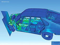
Visualization of how a car deforms in an asymmetrical crash using finite element analysis

Visualization or visualisation (see spelling differences) is any technique for creating images, diagrams, or animations to communicate a message. Visualization through visual imagery has been an effective way to communicate both abstract and concrete ideas since the dawn of humanity. Examples from history include cave paintings, Egyptian hieroglyphs, Greek geometry, and Leonardo da Vinci's revolutionary methods of technical drawing for engineering and scientific purposes.

Visualization today has ever-expanding applications in science, education, engineering (e.g., product visualization), interactive multimedia, medicine, etc. Typical of a visualization application is the field of computer graphics. The invention of computer graphics (and 3D computer graphics) may be the most important development in visualization since the invention of central perspective in the Renaissance period. The development of animation also helped advance visualization.

Overview

The Ptolemy world map, reconstituted from Ptolemy's Geographia (circa 150), indicating the countries of "Serica" and "Sinae" (China) at the extreme right, beyond the island of "Taprobane" (Sri Lanka, oversized) and the "Aurea Chersonesus" (Southeast Asian peninsula)

 

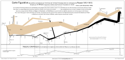
Charles Minard's information graphic of Napoleon's march

The use of visualization to present information is not a new phenomenon. It has been used in maps, scientific drawings, and data plots for over a thousand years. Examples from cartography include Ptolemy's Geographia (2nd century AD), a map of China (1137 AD), and Minard's map (1861) of Napoleon's invasion of Russia a century and a half ago. Most of the concepts learned in devising these images carry over in a straightforward manner to computer visualization. Edward Tufte has written three critically acclaimed books that explain many of these principles.

Computer graphics has from its beginning been used to study scientific problems. However, in its early days the lack of graphics power often limited its usefulness. The recent emphasis on visualization started in 1987 with the publication of Visualization in Scientific Computing, a special issue of Computer Graphics. Since then, there have been several conferences and workshops, co-sponsored by the IEEE Computer Society and ACM SIGGRAPH, devoted to the general topic, and special areas in the field, for example volume visualization.

Most people are familiar with the digital animations produced to present meteorological data during weather reports on television, though few can distinguish between those models of reality and the satellite photos that are also shown on such programs. TV also offers scientific visualizations when it shows computer drawn and animated reconstructions of road or airplane accidents. Some of the most popular examples of scientific visualizations are computer-generated images that show real spacecraft in action, out in the void far beyond Earth, or on other planets. Dynamic forms of visualization, such as educational animation or timelines, have the potential to enhance learning about systems that change over time.

Apart from the distinction between interactive visualizations and animation, the most useful categorization is probably between abstract and model-based scientific visualizations. The abstract visualizations show completely conceptual constructs in 2D or 3D. These generated shapes are completely arbitrary. The model-based visualizations either place overlays of data on real or digitally constructed images of reality or make a digital construction of a real object directly from the scientific data.

Scientific visualization is usually done with specialized software, though there are a few exceptions, noted below. Some of these specialized programs have been released as open source software, having very often its origins in universities, within an academic environment where sharing software tools and giving access to the source code is common. There are also many proprietary software packages of scientific visualization tools.

Models and frameworks for building visualizations include the data flow models popularized by systems such as AVS, IRIS Explorer, and VTK toolkit, and data state models in spreadsheet systems such as the Spreadsheet for Visualization and Spreadsheet for Images.

Applications

Scientific visualization

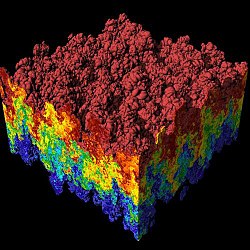
Simulation of a Raleigh–Taylor instability caused by two mixing fluids

 

Main article: Scientific visualization

As a subject in computer science, scientific visualization is the use of interactive, sensory representations, typically visual, of abstract data to reinforce cognition, hypothesis building, and reasoning. Scientific visualization is the transformation, selection, or representation of data from simulations or experiments, with an implicit or explicit geometric structure, to allow the exploration, analysis, and understanding of the data. Scientific visualization focuses and emphasizes the representation of higher order data using primarily graphics and animation techniques. It is a very important part of visualization and maybe the first one, as the visualization of experiments and phenomena is as old as science itself. Traditional areas of scientific visualization are flow visualization, medical visualization, astrophysical visualization, and chemical visualization. There are several different techniques to visualize scientific data, with isosurface reconstruction and direct volume rendering being the more common.

Data visualization

Main article: Data visualization

Data visualization is a related subcategory of visualization dealing with statistical graphics and geospatial data (as in thematic cartography) that is abstracted in schematic form.

Information visualization

Relative average utilization of IPv4

 

Main article: Information visualization

Further information: Information graphics

Information visualization concentrates on the use of computer-supported tools to explore large amount of abstract data. The term "information visualization" was originally coined by the User Interface Research Group at Xerox PARC and included Jock Mackinlay. Practical application of information visualization in computer programs involves selecting, transforming, and representing abstract data in a form that facilitates human interaction for exploration and understanding. Important aspects of information visualization are dynamics of visual representation and the interactivity. Strong techniques enable the user to modify the visualization in real-time, thus affording unparalleled perception of patterns and structural relations in the abstract data in question.

Educational visualization

Educational visualization is using a simulation to create an image of something so it can be taught about. This is very useful when teaching about a topic that is difficult to otherwise see, for example, atomic structure, because atoms are far too small to be studied easily without expensive and difficult to use scientific equipment.

Knowledge visualization

The use of visual representations to transfer knowledge between at least two persons aims to improve the transfer of knowledge by using computer and non-computer-based visualization methods complementarily. Thus properly designed visualization is an important part of not only data analysis but knowledge transfer process, too. Knowledge transfer may be significantly improved using hybrid designs as it enhances information density but may decrease clarity as well. For example, visualization of a 3D scalar field may be implemented using iso-surfaces for field distribution and textures for the gradient of the field. Examples of such visual formats are sketches, diagrams, images, objects, interactive visualizations, information visualization applications, and imaginary visualizations as in stories. While information visualization concentrates on the use of computer-supported tools to derive new insights, knowledge visualization focuses on transferring insights and creating new knowledge in groups. Beyond the mere transfer of facts, knowledge visualization aims to further transfer insights, experiences, attitudes, values, expectations, perspectives, opinions, and predictions by using various complementary visualizations. See also: picture dictionary, visual dictionary

Product visualization

Product visualization involves visualization software technology for the viewing and manipulation of 3D models, technical drawing and other related documentation of manufactured components and large assemblies of products. It is a key part of product lifecycle management. Product visualization software typically provides high levels of photorealism so that a product can be viewed before it is actually manufactured. This supports functions ranging from design and styling to sales and marketing. Technical visualization is an important aspect of product development. Originally technical drawings were made by hand, but with the rise of advanced computer graphics the drawing board has been replaced by computer-aided design (CAD). CAD-drawings and models have several advantages over hand-made drawings such as the possibility of 3-D modeling, rapid prototyping, and simulation. 3D product visualization promises more interactive experiences for online shoppers, but also challenges retailers to overcome hurdles in the production of 3D content, as large-scale 3D content production can be extremely costly and time-consuming.

Visual communication

Visual communication is the communication of ideas through the visual display of information. Primarily associated with two dimensional images, it includes: alphanumerics, art, signs, and electronic resources. Recent research in the field has focused on web design and graphically oriented usability.

Visual analytics

Visual analytics focuses on human interaction with visualization systems as part of a larger process of data analysis. Visual analytics has been defined as "the science of analytical reasoning supported by the interactive visual interface".

Its focus is on human information discourse (interaction) within massive, dynamically changing information spaces. Visual analytics research concentrates on support for perceptual and cognitive operations that enable users to detect the expected and discover the unexpected in complex information spaces.

Technologies resulting from visual analytics find their application in almost all fields, but are being driven by critical needs (and funding) in biology and national security.

Interactivity

See also: Interactive data visualization and Interactive whiteboard

Interactive visualization or interactive visualisation is a branch of graphic visualization in computer science that involves studying how humans interact with computers to create graphic illustrations of information and how this process can be made more efficient.

For a visualization to be considered interactive it must satisfy two criteria:

• Human input: control of some aspect of the visual representation of information, or of the information being represented, must be available to a human, and
• Response time: changes made by the human must be incorporated into the visualization in a timely manner. In general, interactive visualization is considered a soft real-time task.

One particular type of interactive visualization is virtual reality (VR), where the visual representation of information is presented using an immersive display device such as a stereo projector (see stereoscopy). VR is also characterized by the use of a spatial metaphor, where some aspect of the information is represented in three dimensions so that humans can explore the information as if it were present (where instead it was remote), sized appropriately (where instead it was on a much smaller or larger scale than humans can sense directly), or had shape (where instead it might be completely abstract).

Another type of interactive visualization is collaborative visualization, in which multiple people interact with the same computer visualization to communicate their ideas to each other or to explore information cooperatively. Frequently, collaborative visualization is used when people are physically separated. Using several networked computers, the same visualization can be presented to each person simultaneously. The people then make annotations to the visualization as well as communicate via audio (i.e., telephone), video (i.e., a video-conference), or text (i.e., IRC) messages.

Human control of visualization

The Programmer's Hierarchical Interactive Graphics System (PHIGS) was one of the first programmatic efforts at interactive visualization and provided an enumeration of the types of input humans provide. People can:

1. Pick some part of an existing visual representation;
2. Locate a point of interest (which may not have an existing representation);
3. Stroke a path;
4. Choose an option from a list of options;
5. Valuate by inputting a number; and
6. Write by inputting text.

All of these actions require a physical device. Input devices range from the common – keyboards, mice, graphics tablets, trackballs, and touchpads – to the esoteric – wired gloves, boom arms, and even omnidirectional treadmills.

These input actions can be used to control both the information being represented or the way that the information is presented. When the information being presented is altered, the visualization is usually part of a feedback loop. For example, consider an aircraft avionics system where the pilot inputs roll, pitch, and yaw and the visualization system provides a rendering of the aircraft's new attitude. Another example would be a scientist who changes a simulation while it is running in response to a visualization of its current progress. This is called computational steering.

More frequently, the representation of the information is changed rather than the information itself.

Rapid response to human input

Experiments have shown that a delay of more than 20 ms between when input is provided and a visual representation is updated is noticeable by most people. Thus it is desirable for an interactive visualization to provide a rendering based on human input within this time frame. However, when large amounts of data must be processed to create a visualization, this becomes hard or even impossible with current technology. Thus the term "interactive visualization" is usually applied to systems that provide feedback to users within several seconds of input. The term interactive framerate is often used to measure how interactive a visualization is. Framerates measure the frequency with which an image (a frame) can be generated by a visualization system. A framerate of 50 frames per second (frame/s) is considered good while 0.1 frame/s would be considered poor. The use of framerates to characterize interactivity is slightly misleading however, since framerate is a measure of bandwidth while humans are more sensitive to latency. Specifically, it is possible to achieve a good framerate of 50 frame/s but if the images generated refer to changes to the visualization that a person made more than 1 second ago, it will not feel interactive to a person.

The rapid response time required for interactive visualization is a difficult constraint to meet and there are several approaches that have been explored to provide people with rapid visual feedback based on their input. Some include

1. Parallel rendering – where more than one computer or video card is used simultaneously to render an image. Multiple frames can be rendered at the same time by different computers and the results transferred over the network for display on a single monitor. This requires each computer to hold a copy of all the information to be rendered and increases bandwidth, but also increases latency. Also, each computer can render a different region of a single frame and send the results over a network for display. This again requires each computer to hold all of the data and can lead to a load imbalance when one computer is responsible for rendering a region of the screen with more information than other computers. Finally, each computer can render an entire frame containing a subset of the information. The resulting images plus the associated depth buffer can then be sent across the network and merged with the images from other computers. The result is a single frame containing all the information to be rendered, even though no single computer's memory held all of the information. This is called parallel depth compositing and is used when large amounts of information must be rendered interactively.
2. Progressive rendering – where a framerate is guaranteed by rendering some subset of the information to be presented and providing incremental (progressive) improvements to the rendering once the visualization is no longer changing.
3. Level-of-detail (LOD) rendering – where simplified representations of information are rendered to achieve a desired framerate while a person is providing input and then the full representation is used to generate a still image once the person is through manipulating the visualization. One common variant of LOD rendering is subsampling. When the information being represented is stored in a topologically rectangular array (as is common with digital photos, MRI scans, and finite difference simulations), a lower resolution version can easily be generated by skipping n points for each 1 point rendered. Subsampling can also be used to accelerate rendering techniques such as volume visualization that require more than twice the computations for an image twice the size. By rendering a smaller image and then scaling the image to fill the requested screen space, much less time is required to render the same data.
4. Frameless rendering – where the visualization is no longer presented as a time series of images, but as a single image where different regions are updated over time.