Search This Blog

Sunday, September 11, 2022

Least squares

From Wikipedia, the free encyclopedia

The result of fitting a set of data points with a quadratic function
 
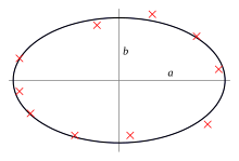
Conic fitting a set of points using least-squares approximation

The method of least squares is a standard approach in regression analysis to approximate the solution of overdetermined systems (sets of equations in which there are more equations than unknowns) by minimizing the sum of the squares of the residuals (a residual being the difference between an observed value and the fitted value provided by a model) made in the results of each individual equation.

The most important application is in data fitting. When the problem has substantial uncertainties in the independent variable (the x variable), then simple regression and least-squares methods have problems; in such cases, the methodology required for fitting errors-in-variables models may be considered instead of that for least squares.

Least squares problems fall into two categories: linear or ordinary least squares and nonlinear least squares, depending on whether or not the residuals are linear in all unknowns. The linear least-squares problem occurs in statistical regression analysis; it has a closed-form solution. The nonlinear problem is usually solved by iterative refinement; at each iteration the system is approximated by a linear one, and thus the core calculation is similar in both cases.

Polynomial least squares describes the variance in a prediction of the dependent variable as a function of the independent variable and the deviations from the fitted curve.

When the observations come from an exponential family with identity as its natural sufficient statistics and mild-conditions are satisfied (e.g. for normal, exponential, Poisson and binomial distributions), standardized least-squares estimates and maximum-likelihood estimates are identical. The method of least squares can also be derived as a method of moments estimator.

The following discussion is mostly presented in terms of linear functions but the use of least squares is valid and practical for more general families of functions. Also, by iteratively applying local quadratic approximation to the likelihood (through the Fisher information), the least-squares method may be used to fit a generalized linear model.

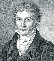
The least-squares method was officially discovered and published by Adrien-Marie Legendre (1805), though it is usually also co-credited to Carl Friedrich Gauss (1795) who contributed significant theoretical advances to the method and may have previously used it in his work.

History

Founding

The method of least squares grew out of the fields of astronomy and geodesy, as scientists and mathematicians sought to provide solutions to the challenges of navigating the Earth's oceans during the Age of Discovery. The accurate description of the behavior of celestial bodies was the key to enabling ships to sail in open seas, where sailors could no longer rely on land sightings for navigation.

The method was the culmination of several advances that took place during the course of the eighteenth century:

  • The combination of different observations as being the best estimate of the true value; errors decrease with aggregation rather than increase, perhaps first expressed by Roger Cotes in 1722.
  • The combination of different observations taken under the same conditions contrary to simply trying one's best to observe and record a single observation accurately. The approach was known as the method of averages. This approach was notably used by Tobias Mayer while studying the librations of the moon in 1750, and by Pierre-Simon Laplace in his work in explaining the differences in motion of Jupiter and Saturn in 1788.
  • The combination of different observations taken under different conditions. The method came to be known as the method of least absolute deviation. It was notably performed by Roger Joseph Boscovich in his work on the shape of the earth in 1757 and by Pierre-Simon Laplace for the same problem in 1799.
  • The development of a criterion that can be evaluated to determine when the solution with the minimum error has been achieved. Laplace tried to specify a mathematical form of the probability density for the errors and define a method of estimation that minimizes the error of estimation. For this purpose, Laplace used a symmetric two-sided exponential distribution we now call Laplace distribution to model the error distribution, and used the sum of absolute deviation as error of estimation. He felt these to be the simplest assumptions he could make, and he had hoped to obtain the arithmetic mean as the best estimate. Instead, his estimator was the posterior median.

The method

The first clear and concise exposition of the method of least squares was published by Legendre in 1805. The technique is described as an algebraic procedure for fitting linear equations to data and Legendre demonstrates the new method by analyzing the same data as Laplace for the shape of the earth. Within ten years after Legendre's publication, the method of least squares had been adopted as a standard tool in astronomy and geodesy in France, Italy, and Prussia, which constitutes an extraordinarily rapid acceptance of a scientific technique.

In 1809 Carl Friedrich Gauss published his method of calculating the orbits of celestial bodies. In that work he claimed to have been in possession of the method of least squares since 1795. This naturally led to a priority dispute with Legendre. However, to Gauss's credit, he went beyond Legendre and succeeded in connecting the method of least squares with the principles of probability and to the normal distribution. He had managed to complete Laplace's program of specifying a mathematical form of the probability density for the observations, depending on a finite number of unknown parameters, and define a method of estimation that minimizes the error of estimation. Gauss showed that the arithmetic mean is indeed the best estimate of the location parameter by changing both the probability density and the method of estimation. He then turned the problem around by asking what form the density should have and what method of estimation should be used to get the arithmetic mean as estimate of the location parameter. In this attempt, he invented the normal distribution.

An early demonstration of the strength of Gauss's method came when it was used to predict the future location of the newly discovered asteroid Ceres. On 1 January 1801, the Italian astronomer Giuseppe Piazzi discovered Ceres and was able to track its path for 40 days before it was lost in the glare of the sun. Based on these data, astronomers desired to determine the location of Ceres after it emerged from behind the sun without solving Kepler's complicated nonlinear equations of planetary motion. The only predictions that successfully allowed Hungarian astronomer Franz Xaver von Zach to relocate Ceres were those performed by the 24-year-old Gauss using least-squares analysis.

In 1810, after reading Gauss's work, Laplace, after proving the central limit theorem, used it to give a large sample justification for the method of least squares and the normal distribution. In 1822, Gauss was able to state that the least-squares approach to regression analysis is optimal in the sense that in a linear model where the errors have a mean of zero, are uncorrelated, and have equal variances, the best linear unbiased estimator of the coefficients is the least-squares estimator. This result is known as the Gauss–Markov theorem.

The idea of least-squares analysis was also independently formulated by the American Robert Adrain in 1808. In the next two centuries workers in the theory of errors and in statistics found many different ways of implementing least squares.

Problem statement

The objective consists of adjusting the parameters of a model function to best fit a data set. A simple data set consists of n points (data pairs) , i = 1, …, n, where is an independent variable and is a dependent variable whose value is found by observation. The model function has the form , where m adjustable parameters are held in the vector . The goal is to find the parameter values for the model that "best" fits the data. The fit of a model to a data point is measured by its residual, defined as the difference between the observed value of the dependent variable and the value predicted by the model:

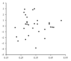
The residuals are plotted against corresponding values. The random fluctuations about indicate a linear model is appropriate.

The least-squares method finds the optimal parameter values by minimizing the sum of squared residuals, :

An example of a model in two dimensions is that of the straight line. Denoting the y-intercept as and the slope as , the model function is given by . See linear least squares for a fully worked out example of this model.

A data point may consist of more than one independent variable. For example, when fitting a plane to a set of height measurements, the plane is a function of two independent variables, x and z, say. In the most general case there may be one or more independent variables and one or more dependent variables at each data point.

To the right is a residual plot illustrating random fluctuations about , indicating that a linear model is appropriate. is an independent, random variable.  

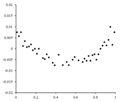
The residuals are plotted against the corresponding values. The parabolic shape of the fluctuations about indicate a parabolic model is appropriate.

If the residual points had some sort of a shape and were not randomly fluctuating, a linear model would not be appropriate. For example, if the residual plot had a parabolic shape as seen to the right, a parabolic model would be appropriate for the data. The residuals for a parabolic model can be calculated via .

Limitations

This regression formulation considers only observational errors in the dependent variable (but the alternative total least squares regression can account for errors in both variables). There are two rather different contexts with different implications:

  • Regression for prediction. Here a model is fitted to provide a prediction rule for application in a similar situation to which the data used for fitting apply. Here the dependent variables corresponding to such future application would be subject to the same types of observation error as those in the data used for fitting. It is therefore logically consistent to use the least-squares prediction rule for such data.
  • Regression for fitting a "true relationship". In standard regression analysis that leads to fitting by least squares there is an implicit assumption that errors in the independent variable are zero or strictly controlled so as to be negligible. When errors in the independent variable are non-negligible, models of measurement error can be used; such methods can lead to parameter estimates, hypothesis testing and confidence intervals that take into account the presence of observation errors in the independent variables. An alternative approach is to fit a model by total least squares; this can be viewed as taking a pragmatic approach to balancing the effects of the different sources of error in formulating an objective function for use in model-fitting.

Solving the least squares problem

The minimum of the sum of squares is found by setting the gradient to zero. Since the model contains m parameters, there are m gradient equations:

and since , the gradient equations become

The gradient equations apply to all least squares problems. Each particular problem requires particular expressions for the model and its partial derivatives.

Linear least squares

A regression model is a linear one when the model comprises a linear combination of the parameters, i.e.,

where the function is a function of .

Letting and putting the independent and dependent variables in matrices and , respectively, we can compute the least squares in the following way. Note that is the set of all data. 

Finding the minimum can be achieved through setting the gradient of the loss to zero and solving for

Finally setting the gradient of the loss to zero and solving for we get: 

Non-linear least squares

There is, in some cases, a closed-form solution to a non-linear least squares problem – but in general there is not. In the case of no closed-form solution, numerical algorithms are used to find the value of the parameters that minimizes the objective. Most algorithms involve choosing initial values for the parameters. Then, the parameters are refined iteratively, that is, the values are obtained by successive approximation:

where a superscript k is an iteration number, and the vector of increments is called the shift vector. In some commonly used algorithms, at each iteration the model may be linearized by approximation to a first-order Taylor series expansion about :

The Jacobian J is a function of constants, the independent variable and the parameters, so it changes from one iteration to the next. The residuals are given by

To minimize the sum of squares of , the gradient equation is set to zero and solved for :

which, on rearrangement, become m simultaneous linear equations, the normal equations:

The normal equations are written in matrix notation as

These are the defining equations of the Gauss–Newton algorithm.

Differences between linear and nonlinear least squares

  • The model function, f, in LLSQ (linear least squares) is a linear combination of parameters of the form The model may represent a straight line, a parabola or any other linear combination of functions. In NLLSQ (nonlinear least squares) the parameters appear as functions, such as and so forth. If the derivatives are either constant or depend only on the values of the independent variable, the model is linear in the parameters. Otherwise the model is nonlinear.
  • Need initial values for the parameters to find the solution to a NLLSQ problem; LLSQ does not require them.
  • Solution algorithms for NLLSQ often require that the Jacobian can be calculated similar to LLSQ. Analytical expressions for the partial derivatives can be complicated. If analytical expressions are impossible to obtain either the partial derivatives must be calculated by numerical approximation or an estimate must be made of the Jacobian, often via finite differences.
  • Non-convergence (failure of the algorithm to find a minimum) is a common phenomenon in NLLSQ.
  • LLSQ is globally concave so non-convergence is not an issue.
  • Solving NLLSQ is usually an iterative process which has to be terminated when a convergence criterion is satisfied. LLSQ solutions can be computed using direct methods, although problems with large numbers of parameters are typically solved with iterative methods, such as the Gauss–Seidel method.
  • In LLSQ the solution is unique, but in NLLSQ there may be multiple minima in the sum of squares.
  • Under the condition that the errors are uncorrelated with the predictor variables, LLSQ yields unbiased estimates, but even under that condition NLLSQ estimates are generally biased.

These differences must be considered whenever the solution to a nonlinear least squares problem is being sought.

Example

Consider a simple example drawn from physics. A spring should obey Hooke's law which states that the extension of a spring y is proportional to the force, F, applied to it.

constitutes the model, where F is the independent variable. In order to estimate the force constant, k, we conduct a series of n measurements with different forces to produce a set of data, , where yi is a measured spring extension. Each experimental observation will contain some error, , and so we may specify an empirical model for our observations,

There are many methods we might use to estimate the unknown parameter k. Since the n equations in the m variables in our data comprise an overdetermined system with one unknown and n equations, we estimate k using least squares. The sum of squares to be minimized is

The least squares estimate of the force constant, k, is given by

We assume that applying force causes the spring to expand. After having derived the force constant by least squares fitting, we predict the extension from Hooke's law.

Uncertainty quantification

In a least squares calculation with unit weights, or in linear regression, the variance on the jth parameter, denoted , is usually estimated with

where the true error variance σ2 is replaced by an estimate, the reduced chi-squared statistic, based on the minimized value of the residual sum of squares (objective function), S. The denominator, n − m, is the statistical degrees of freedom; see effective degrees of freedom for generalizations. C is the covariance matrix.

Statistical testing

If the probability distribution of the parameters is known or an asymptotic approximation is made, confidence limits can be found. Similarly, statistical tests on the residuals can be conducted if the probability distribution of the residuals is known or assumed. We can derive the probability distribution of any linear combination of the dependent variables if the probability distribution of experimental errors is known or assumed. Inferring is easy when assuming that the errors follow a normal distribution, consequently implying that the parameter estimates and residuals will also be normally distributed conditional on the values of the independent variables.

It is necessary to make assumptions about the nature of the experimental errors to test the results statistically. A common assumption is that the errors belong to a normal distribution. The central limit theorem supports the idea that this is a good approximation in many cases.

  • The Gauss–Markov theorem. In a linear model in which the errors have expectation zero conditional on the independent variables, are uncorrelated and have equal variances, the best linear unbiased estimator of any linear combination of the observations, is its least-squares estimator. "Best" means that the least squares estimators of the parameters have minimum variance. The assumption of equal variance is valid when the errors all belong to the same distribution.
  • If the errors belong to a normal distribution, the least-squares estimators are also the maximum likelihood estimators in a linear model.

However, suppose the errors are not normally distributed. In that case, a central limit theorem often nonetheless implies that the parameter estimates will be approximately normally distributed so long as the sample is reasonably large. For this reason, given the important property that the error mean is independent of the independent variables, the distribution of the error term is not an important issue in regression analysis. Specifically, it is not typically important whether the error term follows a normal distribution.

Weighted least squares

"Fanning Out" Effect of Heteroscedasticity
 

A special case of generalized least squares called weighted least squares occurs when all the off-diagonal entries of Ω (the correlation matrix of the residuals) are null; the variances of the observations (along the covariance matrix diagonal) may still be unequal (heteroscedasticity). In simpler terms, heteroscedasticity is when the variance of depends on the value of which causes the residual plot to create a "fanning out" effect towards larger values as seen in the residual plot to the right. On the other hand, homoscedasticity is assuming that the variance of and is equal.   

Relationship to principal components

The first principal component about the mean of a set of points can be represented by that line which most closely approaches the data points (as measured by squared distance of closest approach, i.e. perpendicular to the line). In contrast, linear least squares tries to minimize the distance in the direction only. Thus, although the two use a similar error metric, linear least squares is a method that treats one dimension of the data preferentially, while PCA treats all dimensions equally.

Relationship to Measure Theory

Notable statistician Sara van de Geer used Empirical process theory and the Vapnik-Chervonenkis dimension to prove a least-squares estimator can be interpreted as a measure on the space of square-integrable functions.

Regularization

Tikhonov regularization

In some contexts a regularized version of the least squares solution may be preferable. Tikhonov regularization (or ridge regression) adds a constraint that , the L2-norm of the parameter vector, is not greater than a given value. Equivalently, it may solve an unconstrained minimization of the least-squares penalty with added, where is a constant (this is the Lagrangian form of the constrained problem). In a Bayesian context, this is equivalent to placing a zero-mean normally distributed prior on the parameter vector.

Lasso method

An alternative regularized version of least squares is Lasso (least absolute shrinkage and selection operator), which uses the constraint that , the L1-norm of the parameter vector, is no greater than a given value. (As above, this is equivalent to an unconstrained minimization of the least-squares penalty with added.) In a Bayesian context, this is equivalent to placing a zero-mean Laplace prior distribution on the parameter vector. The optimization problem may be solved using quadratic programming or more general convex optimization methods, as well as by specific algorithms such as the least angle regression algorithm.

One of the prime differences between Lasso and ridge regression is that in ridge regression, as the penalty is increased, all parameters are reduced while still remaining non-zero, while in Lasso, increasing the penalty will cause more and more of the parameters to be driven to zero. This is an advantage of Lasso over ridge regression, as driving parameters to zero deselects the features from the regression. Thus, Lasso automatically selects more relevant features and discards the others, whereas Ridge regression never fully discards any features. Some feature selection techniques are developed based on the LASSO including Bolasso which bootstraps samples, and FeaLect which analyzes the regression coefficients corresponding to different values of to score all the features.

The L1-regularized formulation is useful in some contexts due to its tendency to prefer solutions where more parameters are zero, which gives solutions that depend on fewer variables. For this reason, the Lasso and its variants are fundamental to the field of compressed sensing. An extension of this approach is elastic net regularization.

Oligocene

From Wikipedia, the free encyclopedia

Oligocene
33.9 – 23.03 Ma
Chronology
Etymology
Name formalityFormal
Name ratified1978
Usage information
Celestial bodyEarth
Regional usageGlobal (ICS)
Time scale(s) usedICS Time Scale
Definition
Chronological unitEpoch
Stratigraphic unitSeries
Time span formalityFormal
Lower boundary definitionLAD of Planktonic Foraminifers Hantkenina and Cribrohantkenina
Lower boundary GSSPMassignano quarry section, Massignano, Ancona, Italy
43.5328°N 13.6011°E
GSSP ratified1992
Upper boundary definition
Upper boundary GSSPLemme-Carrosio Section, Carrosio, Italy
44.6589°N 8.8364°E
GSSP ratified1996

The Oligocene ( /ˈɒlɪɡəsn, -ɡ-/ OL-ə-gə-seen, -⁠goh-) is a geologic epoch of the Paleogene Period and extends from about 33.9 million to 23 million years before the present (33.9±0.1 to 23.03±0.05 Ma). As with other older geologic periods, the rock beds that define the epoch are well identified but the exact dates of the start and end of the epoch are slightly uncertain. The name Oligocene was coined in 1854 by the German paleontologist Heinrich Ernst Beyrich from his studies of marine beds in Belgium and Germany. The name comes from the Ancient Greek ὀλίγος (olígos, "few") and καινός (kainós, "new"), and refers to the sparsity of extant forms of molluscs. The Oligocene is preceded by the Eocene Epoch and is followed by the Miocene Epoch. The Oligocene is the third and final epoch of the Paleogene Period.

The Oligocene is often considered an important time of transition, a link between the archaic world of the tropical Eocene and the more modern ecosystems of the Miocene. Major changes during the Oligocene included a global expansion of grasslands, and a regression of tropical broad leaf forests to the equatorial belt.

The start of the Oligocene is marked by a notable extinction event called the Grande Coupure; it featured the replacement of European fauna with Asian fauna, except for the endemic rodent and marsupial families. By contrast, the Oligocene–Miocene boundary is not set at an easily identified worldwide event but rather at regional boundaries between the warmer late Oligocene and the relatively cooler Miocene.

Boundaries and subdivisions

The lower boundary of the Oligocene (its Global Boundary Stratotype Section and Point or GSSP) is placed at the last appearance of the foraminiferan genus Hantkenina in a quarry at Massignano, Italy. However, this GSSP has been criticized as excluding the uppermost part of the type Eocene Priabonian Stage and because it is slightly earlier than important climate shifts that form natural markers for the boundary, such as the global oxygen isotope shift marking the expansion of Antarctic glaciation (the Oi1 event).

The upper boundary of the Oligocene is defined by its GSSP at Carrosio, Italy, which coincides with the first appearance of the foraminiferan Paragloborotalia kugleri and with the base of magnetic polarity chronozone C6Cn.2n.

Oligocene faunal stages from youngest to oldest are:

Chattian or late Oligocene  (27.82–  23.03 mya)
Rupelian or early Oligocene  (33.9–  27.82 mya)

Tectonics and paleogeography

Neotethys during the Oligocene (Rupelian, 33.9–28.4 mya)

During the Oligocene Epoch, the continents continued to drift toward their present positions. Antarctica became more isolated as deep ocean channels were established between Antarctica and Australia and South America. Australia had been very slowly rifting away from West Antarctica since the Jurassic, but the exact timing of the establishment of ocean channels between the two continents remains uncertain. However, one estimate is that a deep channel was in place between the two continents by the end of the early Oligocene. The timing of the formation of the Drake Passage between South America and Australia is also uncertain, with estimates ranging from 49 to 17 mya (early Eocene to Miocene), but oceanic circulation through the Drake Passage may also have been in place by the end of the early Oligocene. This may have been interrupted by a temporary constriction of the Drake Passage from sometime in the middle to late Oligocene (29 to 22 mya) to the middle Miocene (15 mya).

The reorganization of the oceanic tectonic plates of the northeastern Pacific, which had begun in the Paleocene, culminated with the arrival of the Murray and Mendocino Fracture Zones at the North American subduction zone in the Oligocene. This initiated strike-slip movement along the San Andreas Fault and extensional tectonics in the Basin and Range province, ended volcanism south of the Cascades, and produced clockwise rotation of many western North American terranes. The Rocky Mountains were at their peak. A new volcanic arc was established in western North America, far inland from the coast, reaching from central Mexico through the Mogollon-Datil volcanic field to the San Juan volcanic field, then through Utah and Nevada to the ancestral Northern Cascades. Huge ash deposits from these volcanoes created the White River and Arikaree Groups of the High Plains, with their excellent fossil beds.

Between 31 and 26 mya, the Ethiopia-Yemen Continental Flood Basalts were emplaced by the East African large igneous province, which also initiated rifting along the Red Sea and Gulf of Aden.

The Alps were rapidly rising in Europe as the African plate continued to push north into the Eurasian plate, isolating the remnants of the Tethys Sea. Sea levels were lower in the Oligocene than in the early Eocene, exposing large coastal plains in Europe and the Gulf Coast and Atlantic Coast of North America. The Obik Sea, which had separated Europe from Asia, retreated early in the Oligocene, creating a persistent land connection between the continents. There appears to have been a land bridge in the early Oligocene between North America and Europe, since the faunas of the two regions are very similar. However, towards the end of the Oligocene, there was a brief marine incursion in Europe.

The rise of the Himalayas during the Oligocene remains poorly understood. One recent hypothesis is that a separate microcontinent collided with south Asia in the early Eocene, and India itself did not collide with south Asia until the end of the Oligocene. The Tibetan Plateau may have reached nearly its present elevation by the late Oligocene.

The Andes first became a major mountain chain in the Oligocene, as subduction became more direct into the coastline.

Climate

Climate change during the last 65 million years

Climate during the Oligocene reflected a general cooling trend following the Early Eocene Climatic Optimum. This transformed the Earth's climate from a greenhouse to an icehouse climate.

Eocene-Oligocene transition and Oi1 event

The Eocene-Oligocene transition, peaking around 33.5 mya, was a major cooling event and reorganization of the biosphere. The transition is marked by the Oi1 event, in which oxygen isotope ratios decreased by 1.3. About 0.3–0.4 of this is estimated to be due to major expansion of Antarctic ice sheets. The remaining 0.9 to 1.0 was due to about 5 to 6 °C (9 to 10 °F) of global cooling. The transition likely took place in three closely spaced steps over the period from 33.8 to 33.5 mya. By the end of the transition, sea levels had dropped by 105 meters (344 ft), and ice sheets were 25% greater in extent than in the modern world.

The effects of the transition can be seen in the geological record at many locations around the world. Ice volumes rose as temperature and sea levels dropped. Playa lakes of the Tibetan Plateau disappeared at the transition, pointing to cooling and aridification of central Asia. Pollen and spore counts in marine sediments of the Norwegian-Greenland Sea indicate a drop in winter temperatures at high latitudes of about 5 °C (9.0 °F) just prior to the Oi1 event. Borehole dating from the Southeast Faroes drift indicates that deep-ocean circulation from the Arctic Ocean to the North Atlantic Ocean began in the early Oligocene.

The best terrestrial record of Oligocene climate comes from North America, where temperatures dropped by 7 to 11 °C (13 to 20 °F) in the earliest Oligocene. This change is seen from Alaska to the Gulf Coast. Upper Eocene paleosols reflect annual precipitation of over a meter of rain, but early Oligocene precipitation was less than half this. In central North America, the cooling was by 8.2 ± 3.1 °C over a period of 400,000 years, though there is little indication of significant increase in aridity during this interval. Ice-rafted debris in the Norwegian-Greenland Sea indicated that glaciers had appeared in Greenland by the start of the Oligocene.

Continental ice sheets in Antarctica reached sea level during the transition. Glacially rafted debris of early Oligocene age in the Weddell Sea and Kerguelen Plateau, in combination with Oi1 isotope shift, provides unambiguous evidence of a continental ice sheet on Antarctica by the early Oligocene.

The causes of the Eocene-Oligocene transition are not yet fully understood. The timing is wrong for this to be caused either by known impact events or by the volcanic activity on the Ethiopean Plateau. Two other possible drivers of climate change, not mutually exclusive, have been proposed. The first is thermal isolation of the continent of Antarctica by development of the Antarctic Circumpolar Current. Deep sea cores from south of New Zealand suggest that cold deep-sea currents were present by the early Oligocene. However, the timing of this event remains controversial. The other possibility, for which there is considerable evidence, is a drop in atmospheric carbon dioxide levels (pCO2) during the transition. The pCO2 is estimated to have dropped just before the transition, to 760 ppm at the peak of ice sheet growth, then rebounded slightly before resuming a more gradual fall. Climate modeling suggests that glaciation of Antarctica took placed only when pCO2 dropped below a critical threshold value.

Middle Oligocene climate and the Oi2 event

Oligocene climate following the Eocene-Oligocene event is poorly known. There were several pulses of glaciation in middle Oligocene, about the time of the Oi2 oxygen isotope shift. This led to the largest drop of sea level in past 100 million years, by about 75 meters (246 ft). This is reflected in a mid-Oligocene incision of continental shelves and unconformities in marine rocks around the world.

Some evidence suggests that the climate remained warm at high latitudes even as ice sheets experienced cyclical growth and retreat in response to orbital forcing and other climate drivers. Other evidence indicates significant cooling at high latitudes. Part of the difficulty may be that there were strong regional variations in the response to climate shifts. Evidence of a relatively warm Oligocene suggests an enigmatic climate state, neither hothouse nor icehouse.

Late Oligocene warming

The late Oligocene (26.5 to 24 mya) likely saw a warming trend in spite of low pCO2 levels, though this appears to vary by region. However, Antarctica remained heavily glaciated during this warming period. The late Oligocene warming is discernible in pollen counts from the Tibetan Plateau, which also show that the south Asian monsoon had already developed by the late Oligocene.

A deep 400,000-year glaciated Oligocene-Miocene boundary event is recorded at McMurdo Sound and King George Island.

Biosphere

Restoration of Nimravus (far left) and other animals from the Turtle Cove Formation

The early Eocene climate was very warm, with crocodilians and temperate plants thriving above the Arctic Circle. The cooling trend that began in the middle Eocene continued into the Oligocene, bringing the poles well below freezing for the first time in the Phanerozoic. The cooling climate, together with the opening of some land bridges and the closing of others, led to a profound reorganization of the biosphere and loss of taxonomic diversity. Land animals and marine organisms reached a Phanerozoic low in diversity by the late Oligocene, and the temperate forests and jungles of the Eocene were replaced by forest and scrubland. The closing of the Tethys Seaway destroyed its tropical biota.

Flora

The Oi1 event of the Eocene-Oligocene transition covered the continent of Antarctica with ice sheets, leaving Nothofagus and mosses and ferns clinging to life around the periphery of Antarctica in tundra conditions.

Angiosperms continued their expansion throughout the world as tropical and sub-tropical forests were replaced by temperate deciduous forests. Open plains and deserts became more common and grasses expanded from their water-bank habitat in the Eocene moving out into open tracts. The decline in pCO2 favored C4 photosynthesis, which is found only in angiosperms and is particularly characteristic of grasses. However, even at the end of the period, grass was not quite common enough for modern savannas.

In North America, much of the dense forest was replaced by patchy scrubland with riparian forests. Subtropical species dominated with cashews and lychee trees present, and temperate woody plants such as roses, beeches, and pines were common. The legumes spread, while sedges and ferns continued their ascent.

Fauna

Life restoration of Daeodon
 
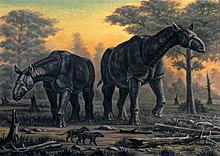
Paraceratherium restored next to Hyaenodon

Most extant mammal families had appeared by the end of the Oligocene. These included primitive three-toed horses, rhinoceroses, camels, deer, and peccaries. Carnivores such as dogs, nimravids (ancestor of cats), bears, weasels, and raccoons began to replace the creodonts that had dominated the Paleocene in the Old World. Rodents and rabbits underwent tremendous diversification due to the increase in suitable habitats for ground-dwelling seed eaters, as habitats for squirrel-like nut- and fruit-eaters diminished. The primates, once present in Eurasia, were reduced in range to Africa and South America. Many groups, such as equids, entelodonts, rhinos, merycoidodonts, and camelids, became more able to run during this time, adapting to the plains that were spreading as the Eocene rainforests receded. Brontotheres died out in the Earliest Oligocene, and creodonts died out outside Africa and the Middle East at the end of the period. Multituberculates, an ancient lineage of primitive mammals that originated back in the Jurassic, also became extinct in the Oligocene, aside from the gondwanatheres.

The Eocene-Oligocene transition in Europe and Asia has been characterized as the Grande Coupure. The lowering of sea levels closed the Turgai Strait across the Obik Sea, which had previously separated Asia from Europe. This allowed Asian mammals, such as rhinoceroses and ruminants, to enter Europe and drive endemic species to extinction. Lesser faunal turnovers occurred simultaneously with the Oi2 event and towards the end of the Oligocene. There was significant diversification of mammals in Eurasia, including the giant indricotheres, that grew up to 6 meters (20 ft) at the shoulder and weighed up to 20 tons. Paraceratherium was one of the largest land mammals ever to walk the Earth. However, the indricotheres were an exception to a general tendency for Oligocene mammals to be much smaller than their Eocene counterparts. The earliest deer, giraffes, pigs, and cattle appeared in the mid-Oligocene in Eurasia. The first felid, Proailurus, originated in Asia during the late Oligocene and spread to Europe.

There was only limited migration between Asia and North America. The cooling of central North America at the Eocene-Oligocene transition resulted in a large turnover of gastropods, amphibians, and reptiles. Mammals were much less affected. Crocodilians and pond turtles replaced by dry land tortoises. Molluscs shifted to more drought-tolerant forms. The White River Fauna of central North America inhabited a semiarid prairie home and included entelodonts like Archaeotherium, camelids (such as Poebrotherium), running rhinoceratoids, three-toed equids (such as Mesohippus), nimravids, protoceratids, and early canids like Hesperocyon. Merycoidodonts, an endemic American group, were very diverse during this time.

Australia and South America became geographically isolated and developed their own distinctive endemic fauna. These included the New World and Old World monkeys. The South American continent was home to animals such as pyrotheres and astrapotheres, as well as litopterns and notoungulates. Sebecosuchians, terror birds, and carnivorous metatheres, like the borhyaenids remained the dominant predators.

Africa was also relative isolated and retained its endemic fauna. These included mastodonts, hyraxes, arsinoitheres, and other archaic forms. Egypt in the Oligocene was an environment of lush forested deltas.

At sea, 97% of marine snail species, 89% of clams, and 50% of echinoderms of the Gulf Coast did not survive past the earliest Oligocene. New species evolved, but the overall diversity diminished. Cold-water mollusks migrated around the Pacific Rim from Alaska and Siberia. The marine animals of Oligocene oceans resembled today's fauna, such as the bivalves. Calcareous cirratulids appeared in the Oligocene. The fossil record of marine mammals is a little spotty during this time, and not as well known as the Eocene or Miocene, but some fossils have been found. The baleen whales and toothed whales had just appeared, and their ancestors, the archaeocete cetaceans began to decrease in diversity due to their lack of echolocation, which was very useful as the water became colder and cloudier. Other factors to their decline could include climate changes and competition with today's modern cetaceans and the requiem sharks, which also appeared in this epoch. Early desmostylians, like Behemotops, are known from the Oligocene. Pinnipeds appeared near the end of the epoch from an otter-like ancestor.

Oceans

The Oligocene sees the beginnings of modern ocean circulation, with tectonic shifts causing the opening and closing of ocean gateways. Cooling of the oceans had already commenced by the Eocene/Oligocene boundary, and they continued to cool as the Oligocene progressed. The formation of permanent Antarctic ice sheets during the early Oligocene and possible glacial activity in the Arctic may have influenced this oceanic cooling, though the extent of this influence is still a matter of some significant dispute.

The effects of oceanic gateways on circulation

The opening and closing of ocean gateways: the opening of the Drake Passage; the opening of the Tasmanian Gateway and the closing of the Tethys seaway; along with the final formation of the GreenlandIcelandFaroes Ridge; played vital parts in reshaping oceanic currents during the Oligocene. As the continents shifted to a more modern configuration, so too did ocean circulation.

The Drake Passage

Eocene-Oligocene circum-Antarctic oceanic changes

The Drake Passage is located between South America and Antarctica. Once the Tasmanian Gateway between Australia and Antarctica opened, all that kept Antarctica from being completely isolated by the Southern Ocean was its connection to South America. As the South American continent moved north, the Drake Passage opened and enabled the formation of the Antarctic Circumpolar Current (ACC), which would have kept the cold waters of Antarctica circulating around that continent and strengthened the formation of Antarctic Bottom Water (ABW). With the cold water concentrated around Antarctica, sea surface temperatures and, consequently, continental temperatures would have dropped. The onset of Antarctic glaciation occurred during the early Oligocene, and the effect of the Drake Passage opening on this glaciation has been the subject of much research. However, some controversy still exists as to the exact timing of the passage opening, whether it occurred at the start of the Oligocene or nearer the end. Even so, many theories agree that at the Eocene/Oligocene (E/O) boundary, a yet shallow flow existed between South America and Antarctica, permitting the start of an Antarctic Circumpolar Current.

Stemming from the issue of when the opening of the Drake Passage took place, is the dispute over how great of an influence the opening of the Drake Passage had on the global climate. While early researchers concluded that the advent of the ACC was highly important, perhaps even the trigger, for Antarctic glaciation and subsequent global cooling, other studies have suggested that the δ18O signature is too strong for glaciation to be the main trigger for cooling. Through study of Pacific Ocean sediments, other researchers have shown that the transition from warm Eocene ocean temperatures to cool Oligocene ocean temperatures took only 300,000 years, which strongly implies that feedbacks and factors other than the ACC were integral to the rapid cooling.

The late Oligocene opening of the Drake Passage

The latest hypothesized time for the opening of the Drake Passage is during the early Miocene. Despite the shallow flow between South America and Antarctica, there was not enough of a deep water opening to allow for significant flow to create a true Antarctic Circumpolar Current. If the opening occurred as late as hypothesized, then the Antarctic Circumpolar Current could not have had much of an effect on early Oligocene cooling, as it would not have existed.

The early Oligocene opening of the Drake Passage

The earliest hypothesized time for the opening of the Drake Passage is around 30 Ma. One of the possible issues with this timing was the continental debris cluttering up the seaway between the two plates in question. This debris, along with what is known as the Shackleton Fracture Zone, has been shown in a recent study to be fairly young, only about 8 million years old. The study concludes that the Drake Passage would be free to allow significant deep water flow by around 31 Ma. This would have facilitated an earlier onset of the Antarctic Circumpolar Current.

Currently, an opening of the Drake Passage during the early Oligocene is favored.

The opening of the Tasman Gateway

The other major oceanic gateway opening during this time was the Tasman, or Tasmanian, depending on the paper, gateway between Australia and Antarctica. The time frame for this opening is less disputed than the Drake Passage and is largely considered to have occurred around 34 Ma. As the gateway widened, the Antarctic Circumpolar Current strengthened.

The Tethys Seaway closing

The Tethys Seaway was not a gateway, but rather a sea in its own right. Its closing during the Oligocene had significant impact on both ocean circulation and climate. The collisions of the African plate with the European plate and of the Indian subcontinent with the Asian plate, cut off the Tethys Seaway that had provided a low-latitude ocean circulation. The closure of Tethys built some new mountains (the Zagros range) and drew down more carbon dioxide from the atmosphere, contributing to global cooling.

Greenland–Iceland–Faroes

The gradual separation of the clump of continental crust and the deepening of the tectonic ridge in the North Atlantic that would become Greenland, Iceland, and the Faroe Islands helped to increase the deep water flow in that area. More information about the evolution of North Atlantic Deep Water will be given a few sections down.

Ocean cooling

Evidence for ocean-wide cooling during the Oligocene exists mostly in isotopic proxies. Patterns of extinction and patterns of species migration can also be studied to gain insight into ocean conditions. For a while, it was thought that the glaciation of Antarctica may have significantly contributed to the cooling of the ocean, however, recent evidence tends to deny this.

Deep water

Reconstruction of Aglaocetus moreni

Isotopic evidence suggests that during the early Oligocene, the main source of deep water was the North Pacific and the Southern Ocean. As the Greenland-Iceland-Faroe Ridge sank and thereby connected the Norwegian–Greenland sea with the Atlantic Ocean, the deep water of the North Atlantic began to come into play as well. Computer models suggest that once this occurred, a more modern in appearance thermo-haline circulation started.

North Atlantic deep water

Evidence for the early Oligocene onset of chilled North Atlantic deep water lies in the beginnings of sediment drift deposition in the North Atlantic, such as the Feni and Southeast Faroe drifts.

South Ocean deep water

The chilling of the South Ocean deep water began in earnest once the Tasmanian Gateway and the Drake Passage opened fully. Regardless of the time at which the opening of the Drake Passage occurred, the effect on the cooling of the Southern Ocean would have been the same.

Impact events

Recorded extraterrestrial impacts:

  • Haughton impact crater, Nunavut, Canada (23 Ma, crater 24 km (15 mi) diameter) (now considered questionable as an Oligocene event; later analyses have concluded the crater dates to 39 Ma, placing the event in the Eocene.)

Supervolcanic explosions

Inequality (mathematics)

From Wikipedia, the free encyclopedia https://en.wikipedia.org/wiki/Inequality...