Adiabatic theorem

From Wikipedia, the free encyclopedia

https://en.wikipedia.org/wiki/Adiabatic_theorem

The adiabatic theorem is a concept in quantum mechanics. Its original form, due to Max Born and Vladimir Fock (1928), was stated as follows:

A physical system remains in its instantaneous eigenstate if a given perturbation is acting on it slowly enough and if there is a gap between the eigenvalue and the rest of the Hamiltonian's spectrum.

In simpler terms, a quantum mechanical system subjected to gradually changing external conditions adapts its functional form, but when subjected to rapidly varying conditions there is insufficient time for the functional form to adapt, so the spatial probability density remains unchanged.

Diabatic vs. adiabatic processes

Comparison

Diabatic	Adiabatic
Rapidly changing conditions prevent the system from adapting its configuration during the process, hence the spatial probability density remains unchanged. Typically there is no eigenstate of the final Hamiltonian with the same functional form as the initial state. The system ends in a linear combination of states that sum to reproduce the initial probability density.	Gradually changing conditions allow the system to adapt its configuration, hence the probability density is modified by the process. If the system starts in an eigenstate of the initial Hamiltonian, it will end in the corresponding eigenstate of the final Hamiltonian.

At some initial time ${\displaystyle t_0}$ a quantum-mechanical system has an energy given by the Hamiltonian ${\displaystyle \hat{H}(t_0)}$; the system is in an eigenstate of ${\displaystyle \hat{H}(t_0)}$ labelled ${\displaystyle \psi (x,t_0)}$. Changing conditions modify the Hamiltonian in a continuous manner, resulting in a final Hamiltonian ${\displaystyle \hat{H}(t_1)}$ at some later time ${\displaystyle t_1}$. The system will evolve according to the time-dependent Schrödinger equation, to reach a final state ${\displaystyle \psi (x,t_1)}$. The adiabatic theorem states that the modification to the system depends critically on the time ${\displaystyle \tau =t_1-t_0}$ during which the modification takes place.

For a truly adiabatic process we require ${\displaystyle \tau \to \mathrm{\infty }}$; in this case the final state ${\displaystyle \psi (x,t_1)}$ will be an eigenstate of the final Hamiltonian ${\displaystyle \hat{H}(t_1)}$, with a modified configuration:

${\displaystyle |\psi (x,t_1){|}^2\ne |\psi (x,t_0){|}^2.}$

The degree to which a given change approximates an adiabatic process depends on both the energy separation between ${\displaystyle \psi (x,t_0)}$ and adjacent states, and the ratio of the interval ${\displaystyle \tau }$ to the characteristic time-scale of the evolution of ${\displaystyle \psi (x,t_0)}$ for a time-independent Hamiltonian, ${\displaystyle {\tau }_{int}=2\pi \hslash /E_0}$, where ${\displaystyle E_0}$ is the energy of ${\displaystyle \psi (x,t_0)}$.

Conversely, in the limit ${\displaystyle \tau \to 0}$ we have infinitely rapid, or diabatic passage; the configuration of the state remains unchanged:

${\displaystyle |\psi (x,t_1){|}^2=|\psi (x,t_0){|}^2.}$

The so-called "gap condition" included in Born and Fock's original definition given above refers to a requirement that the spectrum of ${\displaystyle \hat{H}}$ is discrete and nondegenerate, such that there is no ambiguity in the ordering of the states (one can easily establish which eigenstate of ${\displaystyle \hat{H}(t_1)}$ corresponds to ${\displaystyle \psi (t_0)}$). In 1999 J. E. Avron and A. Elgart reformulated the adiabatic theorem to adapt it to situations without a gap.

Comparison with the adiabatic concept in thermodynamics

The term "adiabatic" is traditionally used in thermodynamics to describe processes without the exchange of heat between system and environment (see adiabatic process), more precisely these processes are usually faster than the timescale of heat exchange. (For example, a pressure wave is adiabatic with respect to a heat wave, which is not adiabatic.) Adiabatic in the context of thermodynamics is often used as a synonym for fast process.

The classical and quantum mechanics definition is closer instead to the thermodynamical concept of a quasistatic process, which are processes that are almost always at equilibrium (i.e. that are slower than the internal energy exchange interactions time scales, namely a "normal" atmospheric heat wave is quasi-static and a pressure wave is not). Adiabatic in the context of Mechanics is often used as a synonym for slow process.

In the quantum world adiabatic means for example that the time scale of electrons and photon interactions is much faster or almost instantaneous with respect to the average time scale of electrons and photon propagation. Therefore, we can model the interactions as a piece of continuous propagation of electrons and photons (i.e. states at equilibrium) plus a quantum jump between states (i.e. instantaneous).

The adiabatic theorem in this heuristic context tells essentially that quantum jumps are preferably avoided and the system tries to conserve the state and the quantum numbers.

The quantum mechanical concept of adiabatic is related to adiabatic invariant, it is often used in the old quantum theory and has no direct relation with heat exchange.

Example systems

Simple pendulum

As an example, consider a pendulum oscillating in a vertical plane. If the support is moved, the mode of oscillation of the pendulum will change. If the support is moved sufficiently slowly, the motion of the pendulum relative to the support will remain unchanged. A gradual change in external conditions allows the system to adapt, such that it retains its initial character. The detailed classical example is available in the Adiabatic invariant page and here.

Quantum harmonic oscillator

Figure 1. Change in the probability density, ${\displaystyle |\psi (t){|}^2}$, of a ground state quantum harmonic oscillator, due to an adiabatic increase in spring constant.

The classical nature of a pendulum precludes a full description of the effects of the adiabatic theorem. As a further example consider a quantum harmonic oscillator as the spring constant ${\displaystyle k}$ is increased. Classically this is equivalent to increasing the stiffness of a spring; quantum-mechanically the effect is a narrowing of the potential energy curve in the system Hamiltonian.

If ${\displaystyle k}$ is increased adiabatically $\left(\frac{dk}{dt}\to 0\right)$ then the system at time ${\displaystyle t}$ will be in an instantaneous eigenstate ${\displaystyle \psi (t)}$ of the current Hamiltonian ${\displaystyle \hat{H}(t)}$, corresponding to the initial eigenstate of ${\displaystyle \hat{H}(0)}$. For the special case of a system like the quantum harmonic oscillator described by a single quantum number, this means the quantum number will remain unchanged. Figure 1 shows how a harmonic oscillator, initially in its ground state, ${\displaystyle n=0}$, remains in the ground state as the potential energy curve is compressed; the functional form of the state adapting to the slowly varying conditions.

For a rapidly increased spring constant, the system undergoes a diabatic process $\left(\frac{dk}{dt}\to \mathrm{\infty }\right)$ in which the system has no time to adapt its functional form to the changing conditions. While the final state must look identical to the initial state ${\displaystyle \left(|\psi (t){|}^2=|\psi (0){|}^2\right)}$ for a process occurring over a vanishing time period, there is no eigenstate of the new Hamiltonian, ${\displaystyle \hat{H}(t)}$, that resembles the initial state. The final state is composed of a linear superposition of many different eigenstates of ${\displaystyle \hat{H}(t)}$ which sum to reproduce the form of the initial state.

Avoided curve crossing

Main article: Avoided crossing

 

Figure 2. An avoided energy-level crossing in a two-level system subjected to an external magnetic field. Note the energies of the diabatic states, ${\displaystyle |1⟩}$ and ${\displaystyle |2⟩}$ and the eigenvalues of the Hamiltonian, giving the energies of the eigenstates ${\displaystyle |{\varphi }_1⟩}$ and ${\displaystyle |{\varphi }_2⟩}$ (the adiabatic states). (Actually, ${\displaystyle |{\varphi }_1⟩}$ and ${\displaystyle |{\varphi }_2⟩}$ should be switched in this picture.)

For a more widely applicable example, consider a 2-level atom subjected to an external magnetic field. The states, labelled ${\displaystyle |1⟩}$ and ${\displaystyle |2⟩}$ using bra–ket notation, can be thought of as atomic angular-momentum states, each with a particular geometry. For reasons that will become clear these states will henceforth be referred to as the diabatic states. The system wavefunction can be represented as a linear combination of the diabatic states:

${\displaystyle |\mathrm{\Psi }⟩=c_1(t)|1⟩+c_2(t)|2⟩.}$

With the field absent, the energetic separation of the diabatic states is equal to ${\displaystyle \hslash {\omega }_0}$; the energy of state ${\displaystyle |1⟩}$ increases with increasing magnetic field (a low-field-seeking state), while the energy of state ${\displaystyle |2⟩}$ decreases with increasing magnetic field (a high-field-seeking state). Assuming the magnetic-field dependence is linear, the Hamiltonian matrix for the system with the field applied can be written

${\displaystyle \mathbf{H}=\left(\begin{array}{cc}\mu B(t)-\hslash {\omega }_0/2& a\\ a^{\ast }& \hslash {\omega }_0/2-\mu B(t)\end{array}\right)}$

where ${\displaystyle \mu }$ is the magnetic moment of the atom, assumed to be the same for the two diabatic states, and ${\displaystyle a}$ is some time-independent coupling between the two states. The diagonal elements are the energies of the diabatic states (${\displaystyle E_1(t)}$ and ${\displaystyle E_2(t)}$), however, as ${\displaystyle \mathbf{H}}$ is not a diagonal matrix, it is clear that these states are not eigenstates of the new Hamiltonian that includes the magnetic field contribution.

The eigenvectors of the matrix ${\displaystyle \mathbf{H}}$ are the eigenstates of the system, which we will label ${\displaystyle |{\varphi }_1(t)⟩}$ and ${\displaystyle |{\varphi }_2(t)⟩}$, with corresponding eigenvalues

$${\displaystyle \begin{array}{rl}{\epsilon }_1(t)& =-\frac{1}{2}\sqrt{4a^2+(\hslash {\omega }_0-2\mu B(t){)}^2}\\ {\epsilon }_2(t)& =+\frac{1}{2}\sqrt{4a^2+(\hslash {\omega }_0-2\mu B(t){)}^2}.\end{array}}$$

It is important to realise that the eigenvalues ${\displaystyle {\epsilon }_1(t)}$ and ${\displaystyle {\epsilon }_2(t)}$ are the only allowed outputs for any individual measurement of the system energy, whereas the diabatic energies ${\displaystyle E_1(t)}$ and ${\displaystyle E_2(t)}$ correspond to the expectation values for the energy of the system in the diabatic states ${\displaystyle |1⟩}$ and ${\displaystyle |2⟩}$.

Figure 2 shows the dependence of the diabatic and adiabatic energies on the value of the magnetic field; note that for non-zero coupling the eigenvalues of the Hamiltonian cannot be degenerate, and thus we have an avoided crossing. If an atom is initially in state ${\displaystyle |{\varphi }_2(t_0)⟩}$ in zero magnetic field (on the red curve, at the extreme left), an adiabatic increase in magnetic field $\left(\frac{dB}{dt}\to 0\right)$ will ensure the system remains in an eigenstate of the Hamiltonian ${\displaystyle |{\varphi }_2(t)⟩}$ throughout the process (follows the red curve). A diabatic increase in magnetic field $\left(\frac{dB}{dt}\to \mathrm{\infty }\right)$ will ensure the system follows the diabatic path (the dotted blue line), such that the system undergoes a transition to state ${\displaystyle |{\varphi }_1(t_1)⟩}$. For finite magnetic field slew rates $\left(0<\frac{dB}{dt}<\mathrm{\infty }\right)$ there will be a finite probability of finding the system in either of the two eigenstates. See below for approaches to calculating these probabilities.

These results are extremely important in atomic and molecular physics for control of the energy-state distribution in a population of atoms or molecules.

Mathematical statement

Under a slowly changing Hamiltonian ${\displaystyle H(t)}$ with instantaneous eigenstates ${\displaystyle |n(t)⟩}$ and corresponding energies ${\displaystyle E_n(t)}$, a quantum system evolves from the initial state

$${\displaystyle |\psi (0)⟩=\sum _n{c}_n(0)|n(0)⟩}$$

to the final state

$${\displaystyle |\psi (t)⟩=\sum _n{c}_n(t)|n(t)⟩,}$$

where the coefficients undergo the change of phase

$${\displaystyle c_n(t)=c_n(0)e^{i{\theta }_n(t)}{e}^{i{\gamma }_n(t)}}$$

with the dynamical phase

$${\displaystyle {\theta }_m(t)=\frac{-1}{\hslash }{\int }_0^t{E}_m(t^{\prime })d{t}^{\prime }}$$

and geometric phase

$${\displaystyle {\gamma }_m(t)=i{\int }_0^t⟨m(t^{\prime })|\dot{m}(t^{\prime })⟩d{t}^{\prime }.}$$

In particular, ${\displaystyle |c_n(t){|}^2=|c_n(0){|}^2}$, so if the system begins in an eigenstate of ${\displaystyle H(0)}$, it remains in an eigenstate of ${\displaystyle H(t)}$ during the evolution with a change of phase only.

Example applications

Often a solid crystal is modeled as a set of independent valence electrons moving in a mean perfectly periodic potential generated by a rigid lattice of ions. With the Adiabatic theorem we can also include instead the motion of the valence electrons across the crystal and the thermal motion of the ions as in the Born–Oppenheimer approximation.

This does explain many phenomena in the scope of:

• thermodynamics: Temperature dependence of specific heat, thermal expansion, melting
• transport phenomena: the temperature dependence of electric resistivity of conductors, the temperature dependence of electric conductivity in insulators, Some properties of low temperature superconductivity
• optics: optic absorption in the infrared for ionic crystals, Brillouin scattering, Raman scattering

Deriving conditions for diabatic vs adiabatic passage

We will now pursue a more rigorous analysis. Making use of bra–ket notation, the state vector of the system at time ${\displaystyle t}$ can be written

${\displaystyle |\psi (t)⟩=\sum _n{c}_n^A(t)e^{-i{E}_{n}t/\hslash }|{\varphi }_n⟩,}$

where the spatial wavefunction alluded to earlier is the projection of the state vector onto the eigenstates of the position operator

${\displaystyle \psi (x,t)=⟨x|\psi (t)⟩.}$

It is instructive to examine the limiting cases, in which ${\displaystyle \tau }$ is very large (adiabatic, or gradual change) and very small (diabatic, or sudden change).

Consider a system Hamiltonian undergoing continuous change from an initial value ${\displaystyle {\hat{H}}_0}$, at time ${\displaystyle t_0}$, to a final value ${\displaystyle {\hat{H}}_1}$, at time ${\displaystyle t_1}$, where ${\displaystyle \tau =t_1-t_0}$. The evolution of the system can be described in the Schrödinger picture by the time-evolution operator, defined by the integral equation

${\displaystyle \hat{U}(t,t_0)=1-\frac{i}{\hslash }{\int }_{t_0}^t\hat{H}(t^{\prime })\hat{U}(t^{\prime },t_0)d{t}^{\prime },}$

which is equivalent to the Schrödinger equation.

${\displaystyle i\hslash \frac{\mathrm{\partial }}{\mathrm{\partial }t}\hat{U}(t,t_0)=\hat{H}(t)\hat{U}(t,t_0),}$

along with the initial condition ${\displaystyle \hat{U}(t_0,t_0)=1}$. Given knowledge of the system wave function at ${\displaystyle t_0}$, the evolution of the system up to a later time ${\displaystyle t}$ can be obtained using

${\displaystyle |\psi (t)⟩=\hat{U}(t,t_0)|\psi (t_0)⟩.}$

The problem of determining the adiabaticity of a given process is equivalent to establishing the dependence of ${\displaystyle \hat{U}(t_1,t_0)}$ on ${\displaystyle \tau }$.

To determine the validity of the adiabatic approximation for a given process, one can calculate the probability of finding the system in a state other than that in which it started. Using bra–ket notation and using the definition ${\displaystyle |0⟩\equiv |\psi (t_0)⟩}$, we have:

${\displaystyle \zeta =⟨0|{\hat{U}}^{†}(t_1,t_0)\hat{U}(t_1,t_0)|0⟩-⟨0|{\hat{U}}^{†}(t_1,t_0)|0⟩⟨0|\hat{U}(t_1,t_0)|0⟩.}$

We can expand ${\displaystyle \hat{U}(t_1,t_0)}$

${\displaystyle \hat{U}(t_1,t_0)=1+\frac{1}{i\hslash }{\int }_{t_0}^{t_1}\hat{H}(t)dt+\frac{1}{(i\hslash {)}^2}{\int }_{t_0}^{t_1}d{t}^{\prime }{\int }_{t_0}^{t^{\prime }}d{t}^{″}\hat{H}(t^{\prime })\hat{H}(t^{″})+\cdots .}$

In the perturbative limit we can take just the first two terms and substitute them into our equation for ${\displaystyle \zeta }$, recognizing that

${\displaystyle \frac{1}{\tau }{\int }_{t_0}^{t_1}\hat{H}(t)dt\equiv \overline{H}}$

is the system Hamiltonian, averaged over the interval ${\displaystyle t_0\to t_1}$, we have:

${\displaystyle \zeta =⟨0|(1+\frac{i}{\hslash }\tau \overline{H})(1-\frac{i}{\hslash }\tau \overline{H})|0⟩-⟨0|(1+\frac{i}{\hslash }\tau \overline{H})|0⟩⟨0|(1-\frac{i}{\hslash }\tau \overline{H})|0⟩.}$

After expanding the products and making the appropriate cancellations, we are left with:

${\displaystyle \zeta =\frac{{\tau }^2}{{\hslash }^2}\left(⟨0|{\overline{H}}^2|0⟩-⟨0|\overline{H}|0⟩⟨0|\overline{H}|0⟩\right),}$

giving

${\displaystyle \zeta =\frac{{\tau }^2\mathrm{\Delta }{\overline{H}}^2}{{\hslash }^2},}$

where ${\displaystyle \mathrm{\Delta }\overline{H}}$ is the root mean square deviation of the system Hamiltonian averaged over the interval of interest.

The sudden approximation is valid when ${\displaystyle \zeta \ll 1}$ (the probability of finding the system in a state other than that in which is started approaches zero), thus the validity condition is given by

${\displaystyle \tau \ll \frac{\hslash }{\mathrm{\Delta }\overline{H}},}$

which is a statement of the time-energy form of the Heisenberg uncertainty principle.

Diabatic passage

In the limit ${\displaystyle \tau \to 0}$ we have infinitely rapid, or diabatic passage:

${\displaystyle \underset{\tau \to 0}{lim}\hat{U}(t_1,t_0)=1.}$

The functional form of the system remains unchanged:

${\displaystyle |⟨x|\psi (t_1)⟩{|}^2={\left|⟨x|\psi (t_0)⟩\right|}^2.}$

This is sometimes referred to as the sudden approximation. The validity of the approximation for a given process can be characterized by the probability that the state of the system remains unchanged:

${\displaystyle P_D=1-\zeta .}$

Adiabatic passage

In the limit ${\displaystyle \tau \to \mathrm{\infty }}$ we have infinitely slow, or adiabatic passage. The system evolves, adapting its form to the changing conditions,

${\displaystyle |⟨x|\psi (t_1)⟩{|}^2\ne |⟨x|\psi (t_0)⟩{|}^2.}$

If the system is initially in an eigenstate of ${\displaystyle \hat{H}(t_0)}$, after a period ${\displaystyle \tau }$ it will have passed into the corresponding eigenstate of ${\displaystyle \hat{H}(t_1)}$.

This is referred to as the adiabatic approximation. The validity of the approximation for a given process can be determined from the probability that the final state of the system is different from the initial state:

${\displaystyle P_A=\zeta .}$

Calculating adiabatic passage probabilities

The Landau–Zener formula

Main article: Landau–Zener formula

In 1932 an analytic solution to the problem of calculating adiabatic transition probabilities was published separately by Lev Landau and Clarence Zener, for the special case of a linearly changing perturbation in which the time-varying component does not couple the relevant states (hence the coupling in the diabatic Hamiltonian matrix is independent of time).

The key figure of merit in this approach is the Landau–Zener velocity:

$${\displaystyle v_{\text{LZ}}=\frac{\frac{\mathrm{\partial }}{\mathrm{\partial }t}|E_2-E_1|}{\frac{\mathrm{\partial }}{\mathrm{\partial }q}|E_2-E_1|}\approx \frac{dq}{dt},}$$

where ${\displaystyle q}$ is the perturbation variable (electric or magnetic field, molecular bond-length, or any other perturbation to the system), and ${\displaystyle E_1}$ and ${\displaystyle E_2}$ are the energies of the two diabatic (crossing) states. A large ${\displaystyle v_{\text{LZ}}}$ results in a large diabatic transition probability and vice versa.

Using the Landau–Zener formula the probability, ${\displaystyle P_{\mathrm{D}}}$, of a diabatic transition is given by

$${\displaystyle \begin{array}{rl}{P}_{\mathrm{D}}& =e^{-2\pi \mathrm{\Gamma }}\\ \mathrm{\Gamma }& =\frac{a^2/\hslash }{\left|\frac{\mathrm{\partial }}{\mathrm{\partial }t}(E_2-E_1)\right|}=\frac{a^2/\hslash }{\left|\frac{dq}{dt}\frac{\mathrm{\partial }}{\mathrm{\partial }q}(E_2-E_1)\right|}\\ & =\frac{a^2}{\hslash |\alpha |}\end{array}}$$

The numerical approach

Main article: Numerical solution of ordinary differential equations

For a transition involving a nonlinear change in perturbation variable or time-dependent coupling between the diabatic states, the equations of motion for the system dynamics cannot be solved analytically. The diabatic transition probability can still be obtained using one of the wide variety of numerical solution algorithms for ordinary differential equations.

The equations to be solved can be obtained from the time-dependent Schrödinger equation:

$${\displaystyle i\hslash {\dot{\underset{\_}{c}}}^A(t)={\mathbf{H}}_A(t){\underset{\_}{c}}^A(t),}$$

where ${\displaystyle {\underset{\_}{c}}^A(t)}$ is a vector containing the adiabatic state amplitudes, ${\displaystyle {\mathbf{H}}_A(t)}$ is the time-dependent adiabatic Hamiltonian, and the overdot represents a time derivative.

Comparison of the initial conditions used with the values of the state amplitudes following the transition can yield the diabatic transition probability. In particular, for a two-state system:

$${\displaystyle P_D=|c_2^A(t_1){|}^2}$$

for a system that began with ${\displaystyle |c_1^A(t_0){|}^2=1}$.

Biome

From Wikipedia, the free encyclopedia
https://en.wikipedia.org/wiki/Biome

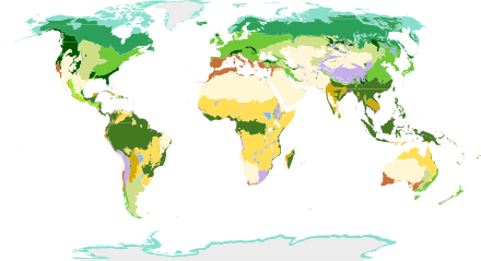
One way of mapping terrestrial (land) biomes around the world

A biome (/ˈbaɪ.oʊm/) is a biogeographical unit consisting of a biological community that has formed in response to the physical environment in which they are found and a shared regional climate.Biomes may span more than one continent. Biome is a broader term than habitat and can comprise a variety of habitats.

While a biome can cover large areas, a microbiome is a mix of organisms that coexist in a defined space on a much smaller scale. For example, the human microbiome is the collection of bacteria, viruses, and other microorganisms that are present on or in a human body.

A 'biota' is the total collection of organisms of a geographic region or a time period. From local geographic scales and instantaneous temporal scales all the way up to whole-planet and whole-timescale spatiotemporal scales. The biotas of the Earth make up the biosphere.

Etymology

The term was suggested in 1916 by Clements, originally as a synonym for biotic community of Möbius (1877). Later, it gained its current definition, based on earlier concepts of phytophysiognomy, formation and vegetation (used in opposition to flora), with the inclusion of the animal element and the exclusion of the taxonomic element of species composition. In 1935, Tansley added the climatic and soil aspects to the idea, calling it ecosystem. The International Biological Program (1964–74) projects popularized the concept of biome.

However, in some contexts, the term biome is used in a different manner. In German literature, particularly in the Walter terminology, the term is used similarly as biotope (a concrete geographical unit), while the biome definition used in this article is used as an international, non-regional, terminology—irrespectively of the continent in which an area is present, it takes the same biome name—and corresponds to his "zonobiome", "orobiome" and "pedobiome" (biomes determined by climate zone, altitude or soil).

In Brazilian literature, the term "biome" is sometimes used as synonym of biogeographic province, an area based on species composition (the term floristic province being used when plant species are considered), or also as synonym of the "morphoclimatic and phytogeographical domain" of Ab'Sáber, a geographic space with subcontinental dimensions, with the predominance of similar geomorphologic and climatic characteristics, and of a certain vegetation form. Both include many biomes in fact.

Classifications

To divide the world into a few ecological zones is difficult, notably because of the small-scale variations that exist everywhere on earth and because of the gradual changeover from one biome to the other. Their boundaries must therefore be drawn arbitrarily and their characterization made according to the average conditions that predominate in them.

A 1978 study on North American grasslands found a positive logistic correlation between evapotranspiration in mm/yr and above-ground net primary production in g/m²/yr. The general results from the study were that precipitation and water use led to above-ground primary production, while solar irradiation and temperature lead to below-ground primary production (roots), and temperature and water lead to cool and warm season growth habit. These findings help explain the categories used in Holdridge's bioclassification scheme (see below), which were then later simplified by Whittaker. The number of classification schemes and the variety of determinants used in those schemes, however, should be taken as strong indicators that biomes do not fit perfectly into the classification schemes created.

Holdridge (1947, 1964) life zones

Holdridge life zone classification scheme. Although conceived as three-dimensional by its originator, it is usually shown as a two-dimensional array of hexagons in a triangular frame.

 

Main article: Holdridge life zones

In 1947, the American botanist and climatologist Leslie Holdridge classified climates based on the biological effects of temperature and rainfall on vegetation under the assumption that these two abiotic factors are the largest determinants of the types of vegetation found in a habitat. Holdridge uses the four axes to define 30 so-called "humidity provinces", which are clearly visible in his diagram. While this scheme largely ignores soil and sun exposure, Holdridge acknowledged that these were important.

Allee (1949) biome-types

The principal biome-types by Allee (1949):

• Tundra
• Taiga
• Deciduous forest
• Grasslands
• Desert
• High plateaus
• Tropical forest
• Minor terrestrial biomes

Kendeigh (1961) biomes

The principal biomes of the world by Kendeigh (1961):

• Terrestrial
  • Temperate deciduous forest
  • Coniferous forest
  • Woodland
  • Chaparral
  • Tundra
  • Grassland
  • Desert
  • Tropical savanna
  • Tropical forest
• Marine
  • Oceanic plankton and nekton
  • Balanoid-gastropod-thallophyte
  • Pelecypod-annelid
  • Coral reef

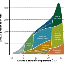
Whittaker (1962, 1970, 1975) biome-types

The distribution of vegetation types as a function of mean annual temperature and precipitation.

Whittaker classified biomes using two abiotic factors: precipitation and temperature. His scheme can be seen as a simplification of Holdridge's; more readily accessible, but missing Holdridge's greater specificity.

Whittaker based his approach on theoretical assertions and empirical sampling. He had previously compiled a review of biome classifications.

Key definitions for understanding Whittaker's scheme

• Physiognomy: sometimes referring to the plants' appearance; or the biome's apparent characteristics, outward features, or appearance of ecological communities or species - including plants.
• Biome: a grouping of terrestrial ecosystems on a given continent that is similar in vegetation structure, physiognomy, features of the environment and characteristics of their animal communities.
• Formation: a major kind of community of plants on a given continent.
• Biome-type: grouping of convergent biomes or formations of different continents, defined by physiognomy.
• Formation-type: a grouping of convergent formations.

Whittaker's distinction between biome and formation can be simplified: formation is used when applied to plant communities only, while biome is used when concerned with both plants and animals. Whittaker's convention of biome-type or formation-type is a broader method to categorize similar communities.

Whittaker's parameters for classifying biome-types

Whittaker used what he called "gradient analysis" of ecocline patterns to relate communities to climate on a worldwide scale. Whittaker considered four main ecoclines in the terrestrial realm.

1. Intertidal levels: The wetness gradient of areas that are exposed to alternating water and dryness with intensities that vary by location from high to low tide
2. Climatic moisture gradient
3. Temperature gradient by altitude
4. Temperature gradient by latitude

Along these gradients, Whittaker noted several trends that allowed him to qualitatively establish biome-types:

• The gradient runs from favorable to the extreme, with corresponding changes in productivity.
• Changes in physiognomic complexity vary with how favorable of an environment exists (decreasing community structure and reduction of stratal differentiation as the environment becomes less favorable).
• Trends in the diversity of structure follow trends in species diversity; alpha and beta species diversities decrease from favorable to extreme environments.
• Each growth-form (i.e. grasses, shrubs, etc.) has its characteristic place of maximum importance along the ecoclines.
• The same growth forms may be dominant in similar environments in widely different parts of the world.

Whittaker summed the effects of gradients (3) and (4) to get an overall temperature gradient and combined this with a gradient (2), the moisture gradient, to express the above conclusions in what is known as the Whittaker classification scheme. The scheme graphs average annual precipitation (x-axis) versus average annual temperature (y-axis) to classify biome-types.

Biome-types

1. Tropical rainforest
2. Tropical seasonal rainforest
   • deciduous
   • semideciduous
3. Temperate giant rainforest
4. Montane rainforest
5. Temperate deciduous forest
6. Temperate evergreen forest
   • needleleaf
   • sclerophyll
7. Subarctic-subalpine needle-leaved forests (taiga)
8. Elfin woodland
9. Thorn forests and woodlands
10. Thorn scrub
11. Temperate woodland
12. Temperate shrublands
    • deciduous
    • heath
    • sclerophyll
    • subalpine-needleleaf
    • subalpine-broadleaf
13. Savanna
14. Temperate grassland
15. Alpine grasslands
16. Tundra
17. Tropical desert
18. Warm-temperate desert
19. Cool temperate desert scrub
20. Arctic-alpine desert
21. Bog
22. Tropical fresh-water swamp forest
23. Temperate fresh-water swamp forest
24. Mangrove swamp
25. Salt marsh
26. Wetland

Goodall (1974–) ecosystem types

The multi-authored series Ecosystems of the World, edited by David W. Goodall, provides a comprehensive coverage of the major "ecosystem types or biomes" on Earth:

1. Terrestrial Ecosystems
   1. Natural Terrestrial Ecosystems
      1. Wet Coastal Ecosystems
      2. Dry Coastal Ecosystems
      3. Polar and Alpine Tundra
      4. Mires: Swamp, Bog, Fen, and Moor
      5. Temperate Deserts and Semi-Deserts
      6. Coniferous Forests
      7. Temperate Deciduous Forests
      8. Natural Grasslands
      9. Heathlands and Related Shrublands
      10. Temperate Broad-Leaved Evergreen Forests
      11. Mediterranean-Type Shrublands
      12. Hot Deserts and Arid Shrublands
      13. Tropical Savannas
      14. Tropical Rain Forest Ecosystems
      15. Wetland Forests
      16. Ecosystems of Disturbed Ground
   2. Managed Terrestrial Ecosystems
      17. Managed Grasslands
      18. Field Crop Ecosystems
      19. Tree Crop Ecosystems
      20. Greenhouse Ecosystems
      21. Bioindustrial Ecosystems
2. Aquatic Ecosystems
   1. Inland Aquatic Ecosystems
      22. River and Stream Ecosystems
      23. Lakes and Reservoirs
   2. Marine Ecosystems
      24. Intertidal and Littoral Ecosystems
      25. Coral Reefs
      26. Estuaries and Enclosed Seas
      27. Ecosystems of the Continental Shelves
      28. Ecosystems of the Deep Ocean
   3. Managed Aquatic Ecosystems
      29. Managed Aquatic Ecosystems
3. Underground Ecosystems
   30. Cave Ecosystems

Walter (1976, 2002) zonobiomes

The eponymously-named Heinrich Walter classification scheme considers the seasonality of temperature and precipitation. The system, also assessing precipitation and temperature, finds nine major biome types, with the important climate traits and vegetation types. The boundaries of each biome correlate to the conditions of moisture and cold stress that are strong determinants of plant form, and therefore the vegetation that defines the region. Extreme conditions, such as flooding in a swamp, can create different kinds of communities within the same biome.

Zonobiome	Zonal soil type	Zonal vegetation type
ZB I. Equatorial, always moist, little temperature seasonality	Equatorial brown clays	Evergreen tropical rainforest
ZB II. Tropical, summer rainy season and cooler “winter” dry season	Red clays or red earths	Tropical seasonal forest, seasonal dry forest, scrub, or savanna
ZB III. Subtropical, highly seasonal, arid climate	Serosemes, sierozemes	Desert vegetation with considerable exposed surface
ZB IV. Mediterranean, winter rainy season and summer drought	Mediterranean brown earths	Sclerophyllous (drought-adapted), frost-sensitive shrublands and woodlands
ZB V. Warm temperate, occasional frost, often with summer rainfall maximum	Yellow or red forest soils, slightly podsolic soils	Temperate evergreen forest, somewhat frost-sensitive
ZB VI. Nemoral, moderate climate with winter freezing	Forest brown earths and grey forest soils	Frost-resistant, deciduous, temperate forest
ZB VII. Continental, arid, with warm or hot summers and cold winters	Chernozems to serozems	Grasslands and temperate deserts
ZB VIII. Boreal, cold temperate with cool summers and long winters	Podsols	Evergreen, frost-hardy, needle-leaved forest (taiga)
ZB IX. Polar, short, cool summers and long, cold winters	Tundra humus soils with solifluction (permafrost soils)	Low, evergreen vegetation, without trees, growing over permanently frozen soils

Schultz (1988) eco-zones

Schultz (1988, 2005) defined nine ecozones (his concept of ecozone is more similar to the concept of biome than to the concept of ecozone of BBC):

1. polar/subpolar zone
2. boreal zone
3. humid mid-latitudes
4. dry mid-latitudes
5. subtropics with winter rain
6. subtropics with year-round rain
7. dry tropics and subtropics
8. tropics with summer rain
9. tropics with year-round rain

Bailey (1989) ecoregions

Robert G. Bailey nearly developed a biogeographical classification system of ecoregions for the United States in a map published in 1976. He subsequently expanded the system to include the rest of North America in 1981, and the world in 1989. The Bailey system, based on climate, is divided into four domains (polar, humid temperate, dry, and humid tropical), with further divisions based on other climate characteristics (subarctic, warm temperate, hot temperate, and subtropical; marine and continental; lowland and mountain).

• 100 Polar Domain
  • 120 Tundra Division (Köppen: Ft)
  • M120 Tundra Division – Mountain Provinces
  • 130 Subarctic Division (Köppen: E)
  • M130 Subarctic Division – Mountain Provinces
• 200 Humid Temperate Domain
  • 210 Warm Continental Division (Köppen: portion of Dcb)
  • M210 Warm Continental Division – Mountain Provinces
  • 220 Hot Continental Division (Köppen: portion of Dca)
  • M220 Hot Continental Division – Mountain Provinces
  • 230 Subtropical Division (Köppen: portion of Cf)
  • M230 Subtropical Division – Mountain Provinces
  • 240 Marine Division (Köppen: Do)
  • M240 Marine Division – Mountain Provinces
  • 250 Prairie Division (Köppen: arid portions of Cf, Dca, Dcb)
  • 260 Mediterranean Division (Köppen: Cs)
  • M260 Mediterranean Division – Mountain Provinces
• 300 Dry Domain
  • 310 Tropical/Subtropical Steppe Division
  • M310 Tropical/Subtropical Steppe Division – Mountain Provinces
  • 320 Tropical/Subtropical Desert Division
  • 330 Temperate Steppe Division
  • 340 Temperate Desert Division
• 400 Humid Tropical Domain
  • 410 Savanna Division
  • 420 Rainforest Division

Olson & Dinerstein (1998) biomes for WWF / Global 200

Terrestrial biomes of the world according to Olson et al. and used by the WWF and Global 200.

 

Main article: Global 200

A team of biologists convened by the World Wildlife Fund (WWF) developed a scheme that divided the world's land area into biogeographic realms (called "ecozones" in a BBC scheme), and these into ecoregions (Olson & Dinerstein, 1998, etc.). Each ecoregion is characterized by a main biome (also called major habitat type).

This classification is used to define the Global 200 list of ecoregions identified by the WWF as priorities for conservation.

For the terrestrial ecoregions, there is a specific EcoID, format XXnnNN (XX is the biogeographic realm, nn is the biome number, NN is the individual number).

Biogeographic realms (terrestrial and freshwater)

• NA: Nearctic
• PA: Palearctic
• AT: Afrotropic
• IM: Indomalaya
• AA: Australasia
• NT: Neotropic
• OC: Oceania
• AN: Antarctic

The applicability of the realms scheme above - based on Udvardy (1975)—to most freshwater taxa is unresolved.

Biogeographic realms (marine)

• Arctic
• Temperate Northern Atlantic
• Temperate Northern Pacific
• Tropical Atlantic
• Western Indo-Pacific
• Central Indo-Pacific
• Eastern Indo-Pacific
• Tropical Eastern Pacific
• Temperate South America
• Temperate Southern Africa
• Temperate Australasia
• Southern Ocean

Biomes (terrestrial)

1. Tropical and subtropical moist broadleaf forests (tropical and subtropical, humid)
2. Tropical and subtropical dry broadleaf forests (tropical and subtropical, semihumid)
3. Tropical and subtropical coniferous forests (tropical and subtropical, semihumid)
4. Temperate broadleaf and mixed forests (temperate, humid)
5. Temperate coniferous forests (temperate, humid to semihumid)
6. Boreal forests/taiga (subarctic, humid)
7. Tropical and subtropical grasslands, savannas, and shrublands (tropical and subtropical, semiarid)
8. Temperate grasslands, savannas, and shrublands (temperate, semiarid)
9. Flooded grasslands and savannas (temperate to tropical, fresh or brackish water inundated)
10. Montane grasslands and shrublands (alpine or montane climate)
11. Tundra (Arctic)
12. Mediterranean forests, woodlands, and scrub or sclerophyll forests (temperate warm, semihumid to semiarid with winter rainfall)
13. Deserts and xeric shrublands (temperate to tropical, arid)
14. Mangrove (subtropical and tropical, salt water inundated)

Biomes (freshwater)

According to the WWF, the following are classified as freshwater biomes:

• Large lakes
• Large river deltas
• Polar freshwaters
• Montane freshwaters
• Temperate coastal rivers
• Temperate floodplain rivers and wetlands
• Temperate upland rivers
• Tropical and subtropical coastal rivers
• Tropical and subtropical floodplain rivers and wetlands
• Tropical and subtropical upland rivers
• Xeric freshwaters and endorheic basins
• Oceanic islands

Biomes (marine)

Biomes of the coastal and continental shelf areas (neritic zone):

• Polar
• Temperate shelves and sea
• Temperate upwelling
• Tropical upwelling
• Tropical coral

Summary of the scheme

• Biosphere
  • Biogeographic realms (terrestrial) (8)
    • Ecoregions (867), each characterized by a main biome type (14)
      • Ecosystems (biotopes)
• Biosphere
  • Biogeographic realms (freshwater) (8)
    • Ecoregions (426), each characterized by a main biome type (12)
      • Ecosystems (biotopes)
• Biosphere
  • Biogeographic realms (marine) (12)
    • (Marine provinces) (62)
      • Ecoregions (232), each characterized by a main biome type (5)
        • Ecosystems (biotopes)

Example:

• Biosphere
  • Biogeographic realm: Palearctic
    • Ecoregion: Dinaric Mountains mixed forests (PA0418); biome type: temperate broadleaf and mixed forests
      • Ecosystem: Orjen, vegetation belt between 1,100 and 1,450 m, Oromediterranean zone, nemoral zone (temperate zone)
        • Biotope: Oreoherzogio-Abietetum illyricae Fuk. (Plant list)
          • Plant: Silver fir (Abies alba)

Other biomes

Marine biomes

Further information: Marine habitats

Pruvot (1896) zones or "systems":

• Littoral zone
• Pelagic zone
• Abyssal zone

Longhurst (1998) biomes:

• Coastal
• Polar
• Trade wind
• Westerly

Other marine habitat types (not covered yet by the Global 200/WWF scheme):

• Open sea
• Deep sea
• Hydrothermal vents
• Cold seeps
• Benthic zone
• Pelagic zone (trades and westerlies)
• Abyssal
• Hadal (ocean trench)
• Littoral/Intertidal zone
• Salt marsh
• Estuaries
• Coastal lagoons/Atoll lagoons
• Kelp forest
• Pack ice

Anthropogenic biomes

Further information: Anthropogenic biome

Humans have altered global patterns of biodiversity and ecosystem processes. As a result, vegetation forms predicted by conventional biome systems can no longer be observed across much of Earth's land surface as they have been replaced by crop and rangelands or cities. Anthropogenic biomes provide an alternative view of the terrestrial biosphere based on global patterns of sustained direct human interaction with ecosystems, including agriculture, human settlements, urbanization, forestry and other uses of land. Anthropogenic biomes offer a way to recognize the irreversible coupling of human and ecological systems at global scales and manage Earth's biosphere and anthropogenic biomes.

Major anthropogenic biomes:

• Dense settlements
• Croplands
• Rangelands
• Forested
• Indoor

Microbial biomes

Main article: Microbiome

Further information: Habitat § Microhabitats

Endolithic biomes

The endolithic biome, consisting entirely of microscopic life in rock pores and cracks, kilometers beneath the surface, has only recently been discovered, and does not fit well into most classification schemes.

Effects of Climate Change

Climate change has the potential to greatly alter the distribution of Earth's biomes. Meaning, biomes around the world could change so much that they would be at risk of becoming new biomes entirely. General frequency models have been a staple in finding out the impact climate change could have on biomes. More specifically, 54% and 22% of global land area will experience climates that correspond to other biomes. 3.6% of land area will experience climates that are completely new or unusual. Average temperatures have risen more than twice the usual amount in both arctic and mountainous biomes. Which leads to the conclusion that artic and mountainous biomes are currently the most vulnerable to climate change. The current reasoning surrounding as to why this is the case are based around the fact that colder environments tend to reflect more sunlight, as a result of the snow and ice covering the ground. Since the annual average temperatures are rising, ice and snow is melting. As a result, albedo is lowered. Keeping a keen eye on terrestrial biomes is important, as they play a crucial role in climate regulation. South American terrestrial biomes have been predicted to go through the same temperature trends as arctic and mountainous biomes. With its annual average temperature continuing to increase, the moisture currently located in forest biomes will dry up.

Nanomotor

From Wikipedia, the free encyclopedia
https://en.wikipedia.org/wiki/Nanomotor

A nanomotor is a molecular or nanoscale device capable of converting energy into movement. It can typically generate forces on the order of piconewtons.

Magnetically controlled Helical Nanomotor moving inside a HeLa cell drawing a pattern 'N'.

While nanoparticles have been utilized by artists for centuries, such as in the famous Lycurgus cup, scientific research into nanotechnology did not come about until recently. In 1959, Richard Feynman gave a famous talk entitled "There's Plenty of Room at the Bottom" at the American Physical Society's conference hosted at Caltech. He went on to wage a scientific bet that no one person could design a motor smaller than 400 µm on any side. The purpose of the bet (as with most scientific bets) was to inspire scientists to develop new technologies, and anyone who could develop a nanomotor could claim the $1,000 USD prize. However, his purpose was thwarted by William McLellan, who fabricated a nanomotor without developing new methods. Nonetheless, Richard Feynman's speech inspired a new generation of scientists to pursue research into nanotechnology.

Kinesin uses protein domain dynamics on nanoscales to walk along a microtubule.

Nanomotors are the focus of research for their ability to overcome microfluidic dynamics present at low Reynold's numbers. Scallop Theory explains that nanomotors must break symmetry to produce motion at low Reynold's numbers. In addition, Brownian motion must be considered because particle-solvent interaction can dramatically impact the ability of a nanomotor to traverse through a liquid. This can pose a significant problem when designing new nanomotors. Current nanomotor research seeks to overcome these problems, and by doing so, can improve current microfluidic devices or give rise to new technologies.

Significant research has been done to overcome microfluidic dynamics at low Reynolds numbers. Now, the more pressing challenge is to overcome issues such as biocompatibility, control on directionality and availability of fuel before nanomotors can be used for theranostic applications within the body.

Nanotube and nanowire motors

Main article: Carbon nanotube nanomotor

In 2004, Ayusman Sen and Thomas E. Mallouk fabricated the first synthetic and autonomous nanomotor. The two-micron long nanomotors were composed of two segments, platinum and gold, that could catalytically react with diluted hydrogen peroxide in water to produce motion. The Au-Pt nanomotors have autonomous, non-Brownian motion that stems from the propulsion via catalytic generation of chemical gradients. As implied, their motion does not require the presence of an external magnetic, electric or optical field to guide their motion. By creating their own local fields, these motors are said to move through self-electrophoresis. Joseph Wang in 2008 was able to dramatically enhance the motion of Au-Pt catalytic nanomotors by incorporating carbon nanotubes into the platinum segment.

Since 2004, different types of nanotube and nanowire based motors have been developed, in addition to nano- and micromotors of different shapes. Most of these motors use hydrogen peroxide as fuel, but some notable exceptions exist.

Metallic microrods (4.3 µm long x 300 nm diameter) can be propelled autonomously in fluids or inside living cells, without chemical fuel, by resonant ultrasound. These rods contain a central Ni stripe that can be steered by an external magnetic field, resulting in "synchronized swimming."

These silver halide and silver-platinum nanomotors are powered by halide fuels, which can be regenerated by exposure to ambient light. Some nanomotors can even be propelled by multiple stimuli, with varying responses. These multi-functional nanowires move in different directions depending on the stimulus (e.g. chemical fuel or ultrasonic power) applied. For example, bimetallic nanomotors have been shown to undergo rheotaxis to move with or against fluid flow by a combination of chemical and acoustic stimuli. In Dresden Germany, rolled-up microtube nanomotors produced motion by harnessing the bubbles in catalytic reactions. Without the reliance on electrostatic interactions, bubble-induced propulsion enables motor movement in relevant biological fluids, but typically still requires toxic fuels such as hydrogen peroxide. This has limited nanomotors' in vitro applications. One in vivo application, however, of microtube motors has been described for the first time by Joseph Wang and Liangfang Zhang using gastric acid as fuel. Recently titanium dioxide has also been identified as a potential candidate for nanomotors due to their corrosion resistance properties and biocompatibility. Future research into catalytical nanomotors holds major promise for important cargo-towing applications, ranging from cell sorting microchip devices to directed drug delivery.

A ribosome is a biological machine that utilizes protein dynamics on nanoscales

Enzymatic nanomotors

Recently, there has been more research into developing enzymatic nanomotors and micropumps. At low Reynold's numbers, single molecule enzymes could act as autonomous nanomotors. Ayusman Sen and Samudra Sengupta demonstrated how self-powered micropumps can enhance particle transportation. This proof-of-concept system demonstrates that enzymes can be successfully utilized as an "engine" in nanomotors and micropumps. It has since been shown that particles themselves will diffuse faster when coated with active enzyme molecules in a solution of their substrate. Further, it has been seen through microfluidic experiments that enzyme molecules will undergo directional swimming up their substrate gradient. This remains the only method of separating enzymes based on activity alone. Additionally, enzymes in cascade have also shown aggregation based on substrate driven chemotaxis. Developing enzyme-driven nanomotors promises to inspire new biocompatible technologies and medical applications. However, several limitations, such as biocompatibility and cellpenetration, have to be overcome for realizing these applications. One of the new biocompatible technologies would be to utilize enzymes for the directional delivery of cargo.

A proposed branch of research is the integration of molecular motor proteins found in living cells into molecular motors implanted in artificial devices. Such a motor protein would be able to move a "cargo" within that device, via protein dynamics, similarly to how kinesin moves various molecules along tracks of microtubules inside cells. Starting and stopping the movement of such motor proteins would involve caging the ATP in molecular structures sensitive to UV light. Pulses of UV illumination would thus provide pulses of movement. DNA nanomachines, based on changes between two molecular conformations of DNA in response to various external triggers, have also been described.

Helical nanomotors

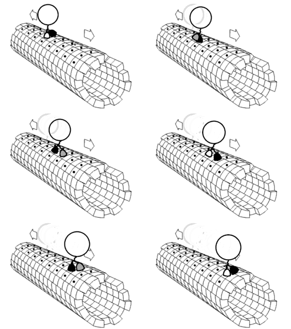
Another interesting direction of research has led to the creation of helical silica particles coated with magnetic materials that can be maneuvered using a rotating magnetic field.

Scanning Electron Microscope image of a Helical nanomotor

Such nanomotors are not dependent on chemical reactions to fuel the propulsion. A triaxial Helmholtz coil can provide directed rotating field in space. Recent works have shown how such nanomotors can be used to measure viscosity of non-newtonian fluids at a resolution of a few microns. This technology promises creation of viscosity map inside cells and the extracellular milieu. Such nanomotors have been demonstrated to move in blood. Recently, researchers have managed to controllably move such nanomotors inside cancer cells allowing them to trace out patterns inside a cell. Nanomotors moving through the tumor microenvironment have demonstrated the presence of sialic acid in the cancer-secreted extracellular matrix.

Current-driven nanomotors (Classical)

In 2003 Fennimore et al. presented the experimental realization of a prototypical current-driven nanomotor. It was based on tiny gold leaves mounted on multiwalled carbon nanotubes, with the carbon layers themselves carrying out the motion. The nanomotor is driven by the electrostatic interaction of the gold leaves with three gate electrodes where alternate currents are applied. Some years later, several other groups showed the experimental realizations of different nanomotors driven by direct currents. The designs typically consisted of organic molecules adsorbed on a metallic surface with a scanning-tunneling-microscope (STM) on top of it. The current flowing from the tip of the STM is used to drive the directional rotation of the molecule or of a part of it. The operation of such nanomotors relies on classical physics and is related to the concept of Brownian motors. These examples of nanomotors are also known as molecular motors.

Quantum effects in current-driven nanomotors

Due to their small size, quantum mechanics plays an important role in some nanomotors. For example, in 2020 Stolz et al. showed the cross-over from classical motion to quantum tunneling in a nanomotor made of a rotating molecule driven by the STM's current. Cold-atom-based ac-driven quantum motors have been explored by several authors. Finally, reverse quantum pumping has been proposed as a general strategy towards the design of nanomotors. In this case, the nanomotors are dubbed as adiabatic quantum motors and it was shown that the quantum nature of electrons can be used to improve the performance of the devices.