Unified neutral theory of biodiversity

From Wikipedia, the free encyclopedia

https://en.wikipedia.org/wiki/Unified_neutral_theory_of_biodiversity 

 

The Unified Neutral Theory of Biodiversity and Biogeography

Author	Stephen P. Hubbell
Country	United States
Language	English
Series	Monographs in Population Biology
Release number	32
Publisher	Princeton University Press
Publication date	2001
Pages	375
ISBN	0-691-02129-5

The unified neutral theory of biodiversity and biogeography (here "Unified Theory" or "UNTB") is a theory and the title of a monograph by ecologist Stephen P. Hubbell. It aims to explain the diversity and relative abundance of species in ecological communities. Like other neutral theories of ecology, Hubbell assumes that the differences between members of an ecological community of trophically similar species are "neutral", or irrelevant to their success. This implies that niche differences do not influence abundance and the abundance of each species follows a random walk. The theory has sparked controversy, and some authors consider it a more complex version of other null models that fit the data better.

"Neutrality" means that at a given trophic level in a food web, species are equivalent in birth rates, death rates, dispersal rates and speciation rates, when measured on a per-capita basis. This can be considered a null hypothesis to niche theory. Hubbell built on earlier neutral models, including Robert MacArthur and E.O. Wilson's theory of island biogeography and Stephen Jay Gould's concepts of symmetry and null models.

An "ecological community" is a group of trophically similar, sympatric species that actually or potentially compete in a local area for the same or similar resources. Under the Unified Theory, complex ecological interactions are permitted among individuals of an ecological community (such as competition and cooperation), provided that all individuals obey the same rules. Asymmetric phenomena such as parasitism and predation are ruled out by the terms of reference; but cooperative strategies such as swarming, and negative interaction such as competing for limited food or light are allowed (so long as all individuals behave alike).

The theory predicts the existence of a fundamental biodiversity constant, conventionally written θ, that appears to govern species richness on a wide variety of spatial and temporal scales.

Saturation

Although not strictly necessary for a neutral theory, many stochastic models of biodiversity assume a fixed, finite community size (total number of individual organisms). There are unavoidable physical constraints on the total number of individuals that can be packed into a given space (although space per se isn't necessarily a resource, it is often a useful surrogate variable for a limiting resource that is distributed over the landscape; examples would include sunlight or hosts, in the case of parasites).

If a wide range of species are considered (say, giant sequoia trees and duckweed, two species that have very different saturation densities), then the assumption of constant community size might not be very good, because density would be higher if the smaller species were monodominant. Because the Unified Theory refers only to communities of trophically similar, competing species, it is unlikely that population density will vary too widely from one place to another.

Hubbell considers the fact that community sizes are constant and interprets it as a general principle: large landscapes are always biotically saturated with individuals. Hubbell thus treats communities as being of a fixed number of individuals, usually denoted by J.

Exceptions to the saturation principle include disturbed ecosystems such as the Serengeti, where saplings are trampled by elephants and Blue wildebeests; or gardens, where certain species are systematically removed.

Species abundances

When abundance data on natural populations are collected, two observations are almost universal:

• The most common species accounts for a substantial fraction of the individuals sampled;
• A substantial fraction of the species sampled are very rare. Indeed, a substantial fraction of the species sampled are singletons, that is, species which are sufficiently rare for only a single individual to have been sampled.

Such observations typically generate a large number of questions. Why are the rare species rare? Why is the most abundant species so much more abundant than the median species abundance?

A non neutral explanation for the rarity of rare species might suggest that rarity is a result of poor adaptation to local conditions. The UNTB suggests that it is not necessary to invoke adaptation or niche differences because neutral dynamics alone can generate such patterns.

Species composition in any community will change randomly with time. Any particular abundance structure will have an associated probability. The UNTB predicts that the probability of a community of J individuals composed of S distinct species with abundances ${\displaystyle n_1}$ for species 1, ${\displaystyle n_2}$ for species 2, and so on up to ${\displaystyle n_S}$ for species S is given by

${\displaystyle Pr(n_1,n_2,\dots ,n_S|\theta ,J)=\frac{J!{\theta }^S}{1^{{\varphi }_1}{2}^{{\varphi }_2}\cdots J^{{\varphi }_J}{\varphi }_1!{\varphi }_2!\cdots {\varphi }_J!{\mathrm{\Pi }}_{k=1}^J(\theta +k-1)}}$

where ${\displaystyle \theta =2J\nu }$ is the fundamental biodiversity number (${\displaystyle \nu }$ is the speciation rate), and ${\displaystyle {\varphi }_i}$ is the number of species that have i individuals in the sample.

This equation shows that the UNTB implies a nontrivial dominance-diversity equilibrium between speciation and extinction.

As an example, consider a community with 10 individuals and three species "a", "b", and "c" with abundances 3, 6 and 1 respectively. Then the formula above would allow us to assess the likelihood of different values of θ. There are thus S = 3 species and ${\displaystyle {\varphi }_1={\varphi }_3={\varphi }_6=1}$, all other ${\displaystyle \varphi }$'s being zero. The formula would give

${\displaystyle Pr(3,6,1|\theta ,10)=\frac{10!{\theta }^3}{1^1\cdot 3^1\cdot 6^1\cdot 1!1!1!\cdot \theta (\theta +1)(\theta +2)\cdots (\theta +9)}}$

which could be maximized to yield an estimate for θ (in practice, numerical methods are used). The maximum likelihood estimate for θ is about 1.1478.

We could have labelled the species another way and counted the abundances being 1,3,6 instead (or 3,1,6, etc. etc.). Logic tells us that the probability of observing a pattern of abundances will be the same observing any permutation of those abundances. Here we would have

${\displaystyle Pr(3;3,6,1)=Pr(3;1,3,6)=Pr(3;3,1,6)}$

and so on.

To account for this, it is helpful to consider only ranked abundances (that is, to sort the abundances before inserting into the formula). A ranked dominance-diversity configuration is usually written as ${\displaystyle Pr(S;r_1,r_2,\dots ,r_s,0,\dots ,0)}$ where ${\displaystyle r_i}$ is the abundance of the ith most abundant species: ${\displaystyle r_1}$ is the abundance of the most abundant, ${\displaystyle r_2}$ the abundance of the second most abundant species, and so on. For convenience, the expression is usually "padded" with enough zeros to ensure that there are J species (the zeros indicating that the extra species have zero abundance).

It is now possible to determine the expected abundance of the ith most abundant species:

${\displaystyle E(r_i)=\sum _{k=1}^C{r}_i(k)\cdot Pr(S;r_1,r_2,\dots ,r_s,0,\dots ,0)}$

where C is the total number of configurations, ${\displaystyle r_i(k)}$ is the abundance of the ith ranked species in the kth configuration, and ${\displaystyle Pr(\dots )}$ is the dominance-diversity probability. This formula is difficult to manipulate mathematically, but relatively simple to simulate computationally.

The model discussed so far is a model of a regional community, which Hubbell calls the metacommunity. Hubbell also acknowledged that on a local scale, dispersal plays an important role. For example, seeds are more likely to come from nearby parents than from distant parents. Hubbell introduced the parameter m, which denotes the probability of immigration in the local community from the metacommunity. If m = 1, dispersal is unlimited; the local community is just a random sample from the metacommunity and the formulas above apply. If m < 1, dispersal is limited and the local community is a dispersal-limited sample from the metacommunity for which different formulas apply.

It has been shown that ${\displaystyle ⟨{\varphi }_n⟩}$, the expected number of species with abundance n, may be calculated by

${\displaystyle \theta \frac{J!}{n!(J-n)!}\frac{\mathrm{\Gamma }(\gamma )}{\mathrm{\Gamma }(J+\gamma )}{\int }_{y=0}^{\gamma }\frac{\mathrm{\Gamma }(n+y)}{\mathrm{\Gamma }(1+y)}\frac{\mathrm{\Gamma }(J-n+\gamma -y)}{\mathrm{\Gamma }(\gamma -y)}\exp (-y\theta /\gamma )dy}$

where θ is the fundamental biodiversity number, J the community size, ${\displaystyle \mathrm{\Gamma }}$ is the gamma function, and ${\displaystyle \gamma =(J-1)m/(1-m)}$. This formula is an approximation. The correct formula is derived in a series of papers, reviewed and synthesized by Etienne and Alonso in 2005:

${\displaystyle \frac{\theta }{(I{)}_J}(\genfrac{}{}{0ex}{}{J}{n}){\int }_0^1(Ix{)}_n(I(1-x){)}_{J-n}\frac{(1-x{)}^{\theta -1}}{x}dx}$

where ${\displaystyle I=(J-1)\ast m/(1-m)}$ is a parameter that measures dispersal limitation.

${\displaystyle ⟨{\varphi }_n⟩}$ is zero for n > J, as there cannot be more species than individuals.

This formula is important because it allows a quick evaluation of the Unified Theory. It is not suitable for testing the theory. For this purpose, the appropriate likelihood function should be used. For the metacommunity this was given above. For the local community with dispersal limitation it is given by:

${\displaystyle Pr(n_1,n_2,\dots ,n_S|\theta ,m,J)=\frac{J!}{\prod _{i=1}^S{n}_i\prod _{j=1}^J{\mathrm{\Phi }}_j!}\frac{{\theta }^S}{(I{)}_J}\sum _{A=S}^{J}K(\overrightarrow{D},A)\frac{I^A}{(\theta {)}_A}}$

Here, the ${\displaystyle K(\overrightarrow{D},A)}$ for ${\displaystyle A=S,...,J}$ are coefficients fully determined by the data, being defined as

${\displaystyle K(\overrightarrow{D},A):=\sum _{\{a_1,...,a_S|\sum _{i=1}^S{a}_i=A\}}\prod _{i=1}^S\frac{\overline{s}\left(n_i,a_i\right)\overline{s}\left(a_i,1\right)}{\overline{s}\left(n_i,1\right)}}$

This seemingly complicated formula involves Stirling numbers and Pochhammer symbols, but can be very easily calculated.

An example of a species abundance curve can be found in Scientific American.

Stochastic modelling of species abundances

UNTB distinguishes between a dispersal-limited local community of size ${\displaystyle J}$ and a so-called metacommunity from which species can (re)immigrate and which acts as a heat bath to the local community. The distribution of species in the metacommunity is given by a dynamic equilibrium of speciation and extinction. Both community dynamics are modelled by appropriate urn processes, where each individual is represented by a ball with a color corresponding to its species. With a certain rate ${\displaystyle r}$ randomly chosen individuals reproduce, i.e. add another ball of their own color to the urn. Since one basic assumption is saturation, this reproduction has to happen at the cost of another random individual from the urn which is removed. At a different rate ${\displaystyle \mu }$ single individuals in the metacommunity are replaced by mutants of an entirely new species. Hubbell calls this simplified model for speciation a point mutation, using the terminology of the Neutral theory of molecular evolution. The urn scheme for the metacommunity of ${\displaystyle J_M}$ individuals is the following.

At each time step take one of the two possible actions :

1. With probability ${\displaystyle (1-\nu )}$ draw an individual at random and replace another random individual from the urn with a copy of the first one.
2. With probability ${\displaystyle \nu }$ draw an individual and replace it with an individual of a new species.

The size ${\displaystyle J_M}$ of the metacommunity does not change. This is a point process in time. The length of the time steps is distributed exponentially. For simplicity one can assume that each time step is as long as the mean time between two changes which can be derived from the reproduction and mutation rates ${\displaystyle r}$ and ${\displaystyle \mu }$. The probability ${\displaystyle \nu }$ is given as ${\displaystyle \nu =\mu /(r+\mu )}$.

The species abundance distribution for this urn process is given by Ewens's sampling formula which was originally derived in 1972 for the distribution of alleles under neutral mutations. The expected number ${\displaystyle S_M(n)}$ of species in the metacommunity having exactly ${\displaystyle n}$ individuals is:

${\displaystyle S_M(n)=\frac{\theta }{n}\frac{\mathrm{\Gamma }(J_M+1)\mathrm{\Gamma }(J_M+\theta -n)}{\mathrm{\Gamma }(J_M+1-n)\mathrm{\Gamma }(J_M+\theta )}}$

where ${\displaystyle \theta =(J_M-1)\nu /(1-\nu )\approx J_M\nu }$ is called the fundamental biodiversity number. For large metacommunities and ${\displaystyle n\ll J_M}$ one recovers the Fisher Log-Series as species distribution.

${\displaystyle S_M(n)\approx \frac{\theta }{n}{\left(\frac{J_M}{J_M+\theta }\right)}^n}$

The urn scheme for the local community of fixed size ${\displaystyle J}$ is very similar to the one for the metacommunity.

At each time step take one of the two actions :

1. With probability ${\displaystyle (1-m)}$ draw an individual at random and replace another random individual from the urn with a copy of the first one.
2. With probability ${\displaystyle m}$ replace a random individual with an immigrant drawn from the metacommunity.

The metacommunity is changing on a much larger timescale and is assumed to be fixed during the evolution of the local community. The resulting distribution of species in the local community and expected values depend on four parameters, ${\displaystyle J}$, ${\displaystyle J_M}$, ${\displaystyle \theta }$ and ${\displaystyle m}$ (or ${\displaystyle I}$) and are derived by Etienne and Alonso (2005), including several simplifying limit cases like the one presented in the previous section (there called ${\displaystyle ⟨{\varphi }_n⟩}$). The parameter ${\displaystyle m}$ is a dispersal parameter. If ${\displaystyle m=1}$ then the local community is just a sample from the metacommunity. For ${\displaystyle m=0}$ the local community is completely isolated from the metacommunity and all species will go extinct except one. This case has been analyzed by Hubbell himself. The case ${\displaystyle 0<m<1}$ is characterized by a unimodal species distribution in a Preston Diagram and often fitted by a log-normal distribution. This is understood as an intermediate state between domination of the most common species and a sampling from the metacommunity, where singleton species are most abundant. UNTB thus predicts that in dispersal limited communities rare species become even rarer. The log-normal distribution describes the maximum and the abundance of common species very well but underestimates the number of very rare species considerably which becomes only apparent for very large sample sizes.

Species-area relationships

The Unified Theory unifies biodiversity, as measured by species-abundance curves, with biogeography, as measured by species-area curves. Species-area relationships show the rate at which species diversity increases with area. The topic is of great interest to conservation biologists in the design of reserves, as it is often desired to harbour as many species as possible.

The most commonly encountered relationship is the power law given by

${\displaystyle S=c{A}^z}$

where S is the number of species found, A is the area sampled, and c and z are constants. This relationship, with different constants, has been found to fit a wide range of empirical data.

From the perspective of Unified Theory, it is convenient to consider S as a function of total community size J. Then ${\displaystyle S=k{J}^z}$ for some constant k, and if this relationship were exactly true, the species area line would be straight on log scales. It is typically found that the curve is not straight, but the slope changes from being steep at small areas, shallower at intermediate areas, and steep at the largest areas.

The formula for species composition may be used to calculate the expected number of species present in a community under the assumptions of the Unified Theory. In symbols

${\displaystyle E\left\{S|\theta ,J\right\}=\frac{\theta }{\theta }+\frac{\theta }{\theta +1}+\frac{\theta }{\theta +2}+\cdots +\frac{\theta }{\theta +J-1}}$

where θ is the fundamental biodiversity number. This formula specifies the expected number of species sampled in a community of size J. The last term, ${\displaystyle \theta /(\theta +J-1)}$, is the expected number of new species encountered when adding one new individual to the community. This is an increasing function of θ and a decreasing function of J, as expected.

By making the substitution ${\displaystyle J=\rho A}$ (see section on saturation above), then the expected number of species becomes ${\displaystyle \mathrm{\Sigma }\theta /(\theta +\rho A-1)}$.

The formula above may be approximated to an integral giving

${\displaystyle S(\theta )=1+\theta \ln \left(1+\frac{J-1}{\theta }\right).}$

This formulation is predicated on a random placement of individuals.

Example

Consider the following (synthetic) dataset of 27 individuals:

a,a,a,a,a,a,a,a,a,a,b,b,b,b,c,c,c,c,d,d,d,d,e,f,g,h,i

There are thus 27 individuals of 9 species ("a" to "i") in the sample. Tabulating this would give:

 a  b  c  d  e  f  g  h  i
10  4  4  4  1  1  1  1  1

indicating that species "a" is the most abundant with 10 individuals and species "e" to "i" are singletons. Tabulating the table gives:

species abundance    1    2    3    4    5    6    7    8    9    10
number of species    5    0    0    3    0    0    0    0    0     1

On the second row, the 5 in the first column means that five species, species "e" through "i", have abundance one. The following two zeros in columns 2 and 3 mean that zero species have abundance 2 or 3. The 3 in column 4 means that three species, species "b", "c", and "d", have abundance four. The final 1 in column 10 means that one species, species "a", has abundance 10.

This type of dataset is typical in biodiversity studies. Observe how more than half the biodiversity (as measured by species count) is due to singletons.

For real datasets, the species abundances are binned into logarithmic categories, usually using base 2, which gives bins of abundance 0–1, abundance 1–2, abundance 2–4, abundance 4–8, etc. Such abundance classes are called octaves; early developers of this concept included F. W. Preston and histograms showing number of species as a function of abundance octave are known as Preston diagrams.

These bins are not mutually exclusive: a species with abundance 4, for example, could be considered as lying in the 2-4 abundance class or the 4-8 abundance class. Species with an abundance of an exact power of 2 (i.e. 2,4,8,16, etc.) are conventionally considered as having 50% membership in the lower abundance class 50% membership in the upper class. Such species are thus considered to be evenly split between the two adjacent classes (apart from singletons which are classified into the rarest category). Thus in the example above, the Preston abundances would be

abundance class 1    1-2   2-4   4-8  8-16
species         5     0    1.5   1.5   1

The three species of abundance four thus appear, 1.5 in abundance class 2–4, and 1.5 in 4–8.

The above method of analysis cannot account for species that are unsampled: that is, species sufficiently rare to have been recorded zero times. Preston diagrams are thus truncated at zero abundance. Preston called this the veil line and noted that the cutoff point would move as more individuals are sampled.

Dynamics

All biodiversity patterns previously described are related to time-independent quantities. For biodiversity evolution and species preservation, it is crucial to compare the dynamics of ecosystems with models (Leigh, 2007). An easily accessible index of the underlying evolution is the so-called species turnover distribution (STD), defined as the probability P(r,t) that the population of any species has varied by a fraction r after a given time t.

A neutral model that can analytically predict both the relative species abundance (RSA) at steady-state and the STD at time t has been presented in Azaele et al. (2006). Within this framework the population of any species is represented by a continuous (random) variable x, whose evolution is governed by the following Langevin equation:

${\displaystyle \dot{x}=b-x/\tau +\sqrt{Dx}\xi (t)}$

where b is the immigration rate from a large regional community, ${\displaystyle -x/\tau }$ represents competition for finite resources and D is related to demographic stochasticity; ${\displaystyle \xi (t)}$ is a Gaussian white noise. The model can also be derived as a continuous approximation of a master equation, where birth and death rates are independent of species, and predicts that at steady-state the RSA is simply a gamma distribution.

From the exact time-dependent solution of the previous equation, one can exactly calculate the STD at time t under stationary conditions:

${\displaystyle P(r,t)=A\frac{\lambda +1}{\lambda }\frac{(e^{t/\tau }{)}^{b/2D}}{1-e^{-t/\tau }}{\left(\frac{\sinh (\frac{t}{2\tau })}{\lambda }\right)}^{\frac{b}{D}+1}{\left(\frac{4{\lambda }^2}{(\lambda +1{)}^2{e}^{t/\tau }-4\lambda }\right)}^{\frac{b}{D}+\frac{1}{2}}.}$

This formula provides good fits of data collected in the Barro Colorado tropical forest from 1990 to 2000. From the best fit one can estimate ${\displaystyle \tau }$ ~ 3500 years with a broad uncertainty due to the relative short time interval of the sample. This parameter can be interpreted as the relaxation time of the system, i.e. the time the system needs to recover from a perturbation of species distribution. In the same framework, the estimated mean species lifetime is very close to the fitted temporal scale ${\displaystyle \tau }$. This suggests that the neutral assumption could correspond to a scenario in which species originate and become extinct on the same timescales of fluctuations of the whole ecosystem.

Testing

The theory has provoked much controversy as it "abandons" the role of ecology when modelling ecosystems. The theory has been criticized as it requires an equilibrium, yet climatic and geographical conditions are thought to change too frequently for this to be attained. Tests on bird and tree abundance data demonstrate that the theory is usually a poorer match to the data than alternative null hypotheses that use fewer parameters (a log-normal model with two tunable parameters, compared to the neutral theory's three), and are thus more parsimonious. The theory also fails to describe coral reef communities, studied by Dornelas et al., and is a poor fit to data in intertidal communities. It also fails to explain why families of tropical trees have statistically highly correlated numbers of species in phylogenetically unrelated and geographically distant forest plots in Central and South America, Africa, and South East Asia.

While the theory has been heralded as a valuable tool for palaeontologists, little work has so far been done to test the theory against the fossil record.

Ecological niche

From Wikipedia, the free encyclopedia

https://en.wikipedia.org/wiki/Ecological_niche 

 

The flightless dung beetle occupies an ecological niche: exploiting animal droppings as a food source.

In ecology, a niche is the match of a species to a specific environmental condition. It describes how an organism or population responds to the distribution of resources and competitors (for example, by growing when resources are abundant, and when predators, parasites and pathogens are scarce) and how it in turn alters those same factors (for example, limiting access to resources by other organisms, acting as a food source for predators and a consumer of prey). "The type and number of variables comprising the dimensions of an environmental niche vary from one species to another [and] the relative importance of particular environmental variables for a species may vary according to the geographic and biotic contexts".

A Grinnellian niche is determined by the habitat in which a species lives and its accompanying behavioral adaptations. An Eltonian niche emphasizes that a species not only grows in and responds to an environment, it may also change the environment and its behavior as it grows. The Hutchinsonian niche uses mathematics and statistics to try to explain how species coexist within a given community.

The concept of ecological niche is central to ecological biogeography, which focuses on spatial patterns of ecological communities. "Species distributions and their dynamics over time result from properties of the species, environmental variation..., and interactions between the two—in particular the abilities of some species, especially our own, to modify their environments and alter the range dynamics of many other species." Alteration of an ecological niche by its inhabitants is the topic of niche construction.

The majority of species exist in a standard ecological niche, sharing behaviors, adaptations, and functional traits similar to the other closely related species within the same broad taxonomic class, but there are exceptions. A premier example of a non-standard niche filling species is the flightless, ground-dwelling kiwi bird of New Zealand, which feeds on worms and other ground creatures, and lives its life in a mammal-like niche. Island biogeography can help explain island species and associated unfilled niches.

Grinnellian niche

The ecological meaning of niche comes from the meaning of niche as a recess in a wall for a statue, which itself is probably derived from the Middle French word nicher, meaning to nest. The term was coined by the naturalist Roswell Hill Johnson but Joseph Grinnell was probably the first to use it in a research program in 1917, in his paper "The niche relationships of the California Thrasher".

The Grinnellian niche concept embodies the idea that the niche of a species is determined by the habitat in which it lives and its accompanying behavioral adaptations. In other words, the niche is the sum of the habitat requirements and behaviors that allow a species to persist and produce offspring. For example, the behavior of the California thrasher is consistent with the chaparral habitat it lives in—it breeds and feeds in the underbrush and escapes from its predators by shuffling from underbrush to underbrush. Its 'niche' is defined by the felicitous complementing of the thrasher's behavior and physical traits (camouflaging color, short wings, strong legs) with this habitat.

The Grinnellian niche can be described as the "needs" niche, or an area that meets the environmental requirements for an organism's survival. Most succulents are native in dry, arid regions like deserts and require large quantities of sun exposure.

Grinnellian niches can be defined by non-interactive (abiotic) variables and environmental conditions on broad scales. Variables of interest in this niche class include average temperature, precipitation, solar radiation, and terrain aspect which have become increasingly accessible across spatial scales. Most literature has focused on Ginnellian niche constructs, often from a climatic perspective, to explain distribution and abundance. Current predictions on species responses to climate change strongly rely on projecting altered environmental conditions on species distributions. However, it is increasingly acknowledged that climate change also influences species interactions and an Eltonian perspective may be advantageous in explaining these processes.

This perspective of niche allows for the existence of both ecological equivalents and empty niches. An ecological equivalent to an organism is an organism from a different taxonomic group exhibiting similar adaptations in a similar habitat, an example being the different succulents found in American and African deserts, cactus and euphorbia, respectively. As another example, the anole lizards of the Greater Antilles are a rare example of convergent evolution, adaptive radiation, and the existence of ecological equivalents: the anole lizards evolved in similar microhabitats independently of each other and resulted in the same ecomorphs across all four islands.

Eltonian niche

In 1927 Charles Sutherland Elton, a British ecologist, defined a niche as follows: "The 'niche' of an animal means its place in the biotic environment, its relations to food and enemies."

Elton classified niches according to foraging activities ("food habits"):

For instance there is the niche that is filled by birds of prey which eat small animals such as shrews and mice. In an oak wood this niche is filled by tawny owls, while in the open grassland it is occupied by kestrels. The existence of this carnivore niche is dependent on the further fact that mice form a definite herbivore niche in many different associations, although the actual species of mice may be quite different.

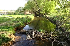
Beaver dam in Hesse, Germany. By exploiting the resource of available wood, beavers are affecting biotic conditions for other species that live within their habitat.

Conceptually, the Eltonian niche introduces the idea of a species' response to and effect on the environment. Unlike other niche concepts, it emphasizes that a species not only grows in and responds to an environment based on available resources, predators, and climatic conditions, but also changes the availability and behavior of those factors as it grows. In an extreme example, beavers require certain resources in order to survive and reproduce, but also construct dams that alter water flow in the river where the beaver lives. Thus, the beaver affects the biotic and abiotic conditions of other species that live in and near the watershed. In a more subtle case, competitors that consume resources at different rates can lead to cycles in resource density that differ between species. Not only do species grow differently with respect to resource density, but their own population growth can affect resource density over time.

Eltonian niches focus on biotic interactions and consumer–resource dynamics (biotic variables) on local scales. Because of the narrow extent of focus, data sets characterizing Eltonian niches typically are in the form of detailed field studies of specific individual phenomena, as the dynamics of this class of niche are difficult to measure at a broad geographic scale. However, the Eltonian niche may be useful in the explanation of a species' endurance of global change. Because adjustments in biotic interactions inevitably change abiotic factors, Eltonian niches can be useful in describing the overall response of a species to new environments.

Hutchinsonian niche

The shape of the bill of this purple-throated carib is complementary to the shape of the flower and coevolved with it, enabling it to exploit the nectar as a resource.

The Hutchinsonian niche is an "n-dimensional hypervolume", where the dimensions are environmental conditions and resources, that define the requirements of an individual or a species to practice its way of life, more particularly, for its population to persist. The "hypervolume" defines the multi-dimensional space of resources (e.g., light, nutrients, structure, etc.) available to (and specifically used by) organisms, and "all species other than those under consideration are regarded as part of the coordinate system."

The niche concept was popularized by the zoologist G. Evelyn Hutchinson in 1957. Hutchinson inquired into the question of why there are so many types of organisms in any one habitat. His work inspired many others to develop models to explain how many and how similar coexisting species could be within a given community, and led to the concepts of 'niche breadth' (the variety of resources or habitats used by a given species), 'niche partitioning' (resource differentiation by coexisting species), and 'niche overlap' (overlap of resource use by different species).

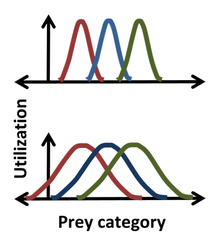
Where three species eat some of the same prey, a statistical picture of each niche shows overlap in resource usage between three species, indicating where competition is strongest.

Statistics were introduced into the Hutchinson niche by Robert MacArthur and Richard Levins using the 'resource-utilization' niche employing histograms to describe the 'frequency of occurrence' as a function of a Hutchinson coordinate. So, for instance, a Gaussian might describe the frequency with which a species ate prey of a certain size, giving a more detailed niche description than simply specifying some median or average prey size. For such a bell-shaped distribution, the position, width and form of the niche correspond to the mean, standard deviation and the actual distribution itself. One advantage in using statistics is illustrated in the figure, where it is clear that for the narrower distributions (top) there is no competition for prey between the extreme left and extreme right species, while for the broader distribution (bottom), niche overlap indicates competition can occur between all species. The resource-utilization approach consists in postulating that not only competition can occur, but also that it does occur, and that overlap in resource utilization directly enables the estimation of the competition coefficients. This postulate, however, can be misguided, as it ignores the impacts that the resources of each category have on the organism and the impacts that the organism has on the resources of each category. For instance, the resource in the overlap region can be non-limiting, in which case there is no competition for this resource despite niche overlap.

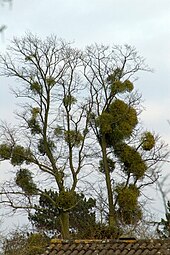
As a hemi-parasitic plant, the mistletoe in this tree exploits its host for nutrients and as a place to grow.

An organism free of interference from other species could use the full range of conditions (biotic and abiotic) and resources in which it could survive and reproduce which is called its fundamental niche. However, as a result of pressure from, and interactions with, other organisms (i.e. inter-specific competition) species are usually forced to occupy a niche that is narrower than this, and to which they are mostly highly adapted; this is termed the realized niche. Hutchinson used the idea of competition for resources as the primary mechanism driving ecology, but overemphasis upon this focus has proved to be a handicap for the niche concept. In particular, overemphasis upon a species' dependence upon resources has led to too little emphasis upon the effects of organisms on their environment, for instance, colonization and invasions.

The term "adaptive zone" was coined by the paleontologist George Gaylord Simpson to explain how a population could jump from one niche to another that suited it, jump to an 'adaptive zone', made available by virtue of some modification, or possibly a change in the food chain, that made the adaptive zone available to it without a discontinuity in its way of life because the group was 'pre-adapted' to the new ecological opportunity.

Hutchinson's "niche" (a description of the ecological space occupied by a species) is subtly different from the "niche" as defined by Grinnell (an ecological role, that may or may not be actually filled by a species—see vacant niches).

A niche is a very specific segment of ecospace occupied by a single species. On the presumption that no two species are identical in all respects (called Hardin's 'axiom of inequality') and the competitive exclusion principle, some resource or adaptive dimension will provide a niche specific to each species. Species can however share a 'mode of life' or 'autecological strategy' which are broader definitions of ecospace. For example, Australian grasslands species, though different from those of the Great Plains grasslands, exhibit similar modes of life.

Once a niche is left vacant, other organisms can fill that position. For example, the niche that was left vacant by the extinction of the tarpan has been filled by other animals (in particular a small horse breed, the konik). Also, when plants and animals are introduced into a new environment, they have the potential to occupy or invade the niche or niches of native organisms, often outcompeting the indigenous species. Introduction of non-indigenous species to non-native habitats by humans often results in biological pollution by the exotic or invasive species.

The mathematical representation of a species' fundamental niche in ecological space, and its subsequent projection back into geographic space, is the domain of niche modelling.

Contemporary niche theory

Contemporary niche theory (also called "classic niche theory" in some contexts) is a framework that was originally designed to reconcile different definitions of niches (see Grinnellian, Eltonian, and Hutchinsonian definitions above), and to help explain the underlying processes that affect Lotka-Volterra relationships within an ecosystem. The framework centers around "consumer-resource models" which largely split a given ecosystem into resources (e.g. sunlight or available water in soil) and consumers (e.g. any living thing, including plants and animals), and attempts to define the scope of possible relationships that could exist between the two groups.

In contemporary niche theory, the "impact niche" is defined as the combination of effects that a given consumer has on both a). the resources that it uses, and b). the other consumers in the ecosystem. Therefore, the impact niche is equivalent to the Eltonian niche since both concepts are defined by the impact of a given species on its environment.

The range of environmental conditions where a species can successfully survive and reproduce (i.e. the Hutchinsonian definition of a realized niche) is also encompassed under contemporary niche theory, termed the "requirement niche". The requirement niche is bounded by both the availability of resources as well as the effects of coexisting consumers (e.g. competitors and predators).

Coexistence under contemporary niche theory

Contemporary niche theory provides three requirements that must be met in order for two species (consumers) to coexist:

1. The requirement niches of both consumers must overlap.
2. Each consumer must outcompete the other for the resource that it needs most. For example, if two plants (P1 and P2) are competing for nitrogen and phosphorus in a given ecosystem, they will only coexist if they are limited by different resources (P1 is limited by nitrogen and P2 is limited by phosphorus, perhaps) and each species must outcompete the other species to get that resource (P1 needs to be better at obtaining nitrogen and P2 needs to be better at obtaining phosphorus). Intuitively, this makes sense from an inverse perspective: If both consumers are limited by the same resource, one of the species will ultimately be the better competitor, and only that species will survive. Furthermore, if P1 was outcompeted for the nitrogen (the resource it needed most) it would not survive. Likewise, if P2 was outcompeted for phosphorus, it would not survive.
3. The availability of the limiting resources (nitrogen and phosphorus in the above example) in the environment are equivalent.

These requirements are interesting and controversial because they require any two species to share a certain environment (have overlapping requirement niches) but fundamentally differ the ways that they use (or "impact") that environment. These requirements have repeatedly been violated by nonnative (i.e. introduced and invasive) species, which often coexist with new species in their nonnative ranges, but do not appear to be constricted these requirements. In other words, contemporary niche theory predicts that species will be unable to invade new environments outside of their requirement (i.e. realized) niche, yet many examples of this are well-documented. Additionally, contemporary niche theory predicts that species will be unable to establish in environments where other species already consume resources in the same ways as the incoming species, however examples of this are also numerous.

Niche and Geographic Range

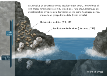
Diagram representation of the effects of competitive exclusion on the barnacle Chthamalus stellatus in the intertidal zone. The fundamental and realized geographic ranges of C. stellatus are represented by the dark blue and light blue bars, respectively.

The geographic range of a species can be viewed as a spatial reflection of its niche, along with characteristics of the geographic template and the species that influence its potential to colonize. The fundamental geographic range of a species is the area it occupies in which environmental conditions are favorable, without restriction from barriers to disperse or colonize. A species will be confined to its realized geographic range when confronting biotic interactions or abiotic barriers that limit dispersal, a more narrow subset of its larger fundamental geographic range.

An early study on ecological niches conducted by Joseph H. Connell analyzed the environmental factors that limit the range of a barnacle (Chthamalus stellatus) on Scotland's Isle of Cumbrae. In his experiments, Connell described the dominant features of C. stellatus niches and provided explanation for their distribution on intertidal zone of the rocky coast of the Isle. Connell described the upper portion of C. stellatus's range is limited by the barnacle's ability to resist dehydration during periods of low tide. The lower portion of the range was limited by interspecific interactions, namely competition with a cohabiting barnacle species and predation by a snail. By removing the competing B. balanoides, Connell showed that C. stellatus was able to extend the lower edge of its realized niche in the absence of competitive exclusion. These experiments demonstrate how biotic and abiotic factors limit the distribution of an organism.

Parameters

The different dimensions, or plot axes, of a niche represent different biotic and abiotic variables. These factors may include descriptions of the organism's life history, habitat, trophic position (place in the food chain), and geographic range. According to the competitive exclusion principle, no two species can occupy the same niche in the same environment for a long time. The parameters of a realized niche are described by the realized niche width of that species. Some plants and animals, called specialists, need specific habitats and surroundings to survive, such as the spotted owl, which lives specifically in old growth forests. Other plants and animals, called generalists, are not as particular and can survive in a range of conditions, for example the dandelion.