Economic equilibrium

From Wikipedia, the free encyclopedia

https://en.wikipedia.org/wiki/Economic_equilibrium 

 

Economic equilibrium
A solution concept in game theory
Relationship
Subset of	Equilibrium, Free market
Superset of	Competitive equilibrium, Nash equilibrium, Intertemporal equilibrium, Recursive competitive equilibrium
Significance

Used for	mostly Perfect competition, but also some Imperfect competition

In economics, economic equilibrium is a situation in which economic forces such as supply and demand are balanced and in the absence of external influences the (equilibrium) values of economic variables will not change. For example, in the standard text perfect competition, equilibrium occurs at the point at which quantity demanded and quantity supplied are equal.

Market equilibrium in this case is a condition where a market price is established through competition such that the amount of goods or services sought by buyers is equal to the amount of goods or services produced by sellers. This price is often called the competitive price or market clearing price and will tend not to change unless demand or supply changes, and quantity is called the "competitive quantity" or market clearing quantity. But the concept of equilibrium in economics also applies to imperfectly competitive markets, where it takes the form of a Nash equilibrium.

Understanding economic equilibrium

An economic equilibrium is a situation when the economic agent cannot change the situation by adopting any strategy. To fully grasp the concept of economic equilibrium, it must be highlighted that it has been borrowed from the physical sciences. Take a system where physical forces are balanced for instance.This economically interpreted means no further change ensues.

Properties of equilibrium

Three basic properties of equilibrium in general have been proposed by Huw Dixon. These are:

Equilibrium property P1: The behavior of agents is consistent.

Equilibrium property P2: No agent has an incentive to change its behavior.

Equilibrium property P3: Equilibrium is the outcome of some dynamic process (stability).

Example: competitive equilibrium

Competitive Equilibrium: Price equates supply and demand.

• P – price
• Q – quantity demanded and supplied
• S – supply curve
• D – demand curve
• P₀ – equilibrium price
• A – excess demand – when P<P₀
• B – excess supply – when P>P₀

In a competitive equilibrium, supply equals demand. Property P1 is satisfied, because at the equilibrium price the amount supplied is equal to the amount demanded. Property P2 is also satisfied. Demand is chosen to maximize utility given the market price: no one on the demand side has any incentive to demand more or less at the prevailing price. Likewise supply is determined by firms maximizing their profits at the market price: no firm will want to supply any more or less at the equilibrium price. Hence, agents on neither the demand side nor the supply side will have any incentive to alter their actions.

To see whether Property P3 is satisfied, consider what happens when the price is above the equilibrium. In this case there is an excess supply, with the quantity supplied exceeding that demanded. This will tend to put downward pressure on the price to make it return to equilibrium. Likewise where the price is below the equilibrium point there is a shortage in supply leading to an increase in prices back to equilibrium. Not all equilibria are "stable" in the sense of equilibrium property P3. It is possible to have competitive equilibria that are unstable. However, if an equilibrium is unstable, it raises the question of reaching it. Even if it satisfies properties P1 and P2, the absence of P3 means that the market can only be in the unstable equilibrium if it starts off there.

In most simple microeconomic stories of supply and demand a static equilibrium is observed in a market; however, economic equilibrium can be also dynamic. Equilibrium may also be economy-wide or general, as opposed to the partial equilibrium of a single market. Equilibrium can change if there is a change in demand or supply conditions. For example, an increase in supply will disrupt the equilibrium, leading to lower prices. Eventually, a new equilibrium will be attained in most markets. Then, there will be no change in price or the amount of output bought and sold — until there is an exogenous shift in supply or demand (such as changes in technology or tastes). That is, there are no endogenous forces leading to the price or the quantity.

Example: monopolist equilibrium

In a monopoly, marginal revenue (MR) equals marginal cost (MC). The equilibrium quantity is obtained from where MR and MC intersect and the equilibrium price can be found on the demand curve where MR = MC. Property P1 is not satisfied because the amount demand and the amount supplied at the equilibrium price are not equal. Property P2 is not satisfied. Because the monopolist's profit-maximizing quantity is different from the socially-maximizing quantity, consumer's have an incentive to demand more at the equilibrium price. However, at the market price, monopolists maximize their profits so they have no incentive to change their price. Therefore, agents on the demand side have an incentive to alter their actions while the agents on the supply side do not have any incentive to alter their actions.

In order to determine if Property P3 is satisfied, the same situations used to determine P3 in a competitive equilibrium can be used. When there is an excess in supply, monopolists will realize that the equilibrium is not at the profit-maximizing quantity and will put upward pressure on the price to make it return to equilibrium. This is the same case when the price is above the equilibrium and the shortage in supply leads the monopolist to decrease the supply to return to the profit-maximizing quantity. Therefore the equilibrium is the result of stability.

Example: Nash equilibrium

Further information: Nash equilibrium and Cournot model

Equilibrium quantities as a solution to two reaction functions in Cournot duopoly. Firm 1's reaction function q1=R1(q2) gives its optimal output q1 to a given output q2 of firm 2. Likewise, firm 2's reaction function q2=R2(q1). The Cournot-Nash equilibrium occurs where the two reaction functions intersect and both firms are choosing the optimal output given the output of the other firm.

The Nash equilibrium is widely used in economics as the main alternative to competitive equilibrium. It is used whenever there is a strategic element to the behavior of agents and the "price taking" assumption of competitive equilibrium is inappropriate. The first use of the Nash equilibrium was in the Cournot duopoly as developed by Antoine Augustin Cournot in his 1838 book. Both firms produce a homogenous product: given the total amount supplied by the two firms, the (single) industry price is determined using the demand curve. This determines the revenues of each firm (the industry price times the quantity supplied by the firm). The profit of each firm is then this revenue minus the cost of producing the output. Clearly, there is a strategic interdependence between the two firms. If one firm varies its output, this will in turn affect the market price and so the revenue and profits of the other firm. We can define the payoff function which gives the profit of each firm as a function of the two outputs chosen by the firms. Cournot assumed that each firm chooses its own output to maximize its profits given the output of the other firm. The Nash equilibrium occurs when both firms are producing the outputs which maximize their own profit given the output of the other firm.

In terms of the equilibrium properties, we can see that P2 is satisfied: in a Nash equilibrium, neither firm has an incentive to deviate from the Nash equilibrium given the output of the other firm. P1 is satisfied since the payoff function ensures that the market price is consistent with the outputs supplied and that each firms profits equal revenue minus cost at this output.

Is the equilibrium stable as required by P3? Cournot himself argued that it was stable using the stability concept implied by best response dynamics. The reaction function for each firm gives the output which maximizes profits (best response) in terms of output for a firm in terms of a given output of the other firm. In the standard Cournot model this is downward sloping: if the other firm produces a higher output, the best response involves producing less. Best response dynamics involves firms starting from some arbitrary position and then adjusting output to their best-response to the previous output of the other firm. So long as the reaction functions have a slope of less than -1, this will converge to the Nash equilibrium. However, this stability story is open to much criticism. As Dixon argues: "The crucial weakness is that, at each step, the firms behave myopically: they choose their output to maximize their current profits given the output of the other firm, but ignore the fact that the process specifies that the other firm will adjust its output...". There are other concepts of stability that have been put forward for the Nash equilibrium, evolutionary stability for example.

Example: Walrasian equilibrium in a Power economy

Walrasian Equilibrium Prices

A fictional auctioneer calls out prices. Consumers and firms report honestly their demands and supplies.

When Net Demand = [Demand - Supply] is zero, the auctioneer's job is done. The prices are market clearing prices.

Special case: An island economy.

Supply

Consumers a and b survive by consuming coconuts that fall from the palm trees, x, and crayfish, y, trapped in the lagoon. This yields 1 basketful per day of each commodity.

Only the price ratio p = p₁/p₂ matters so the auctioneer only has to call out one price.

There is one daily basketful of each commodity. Therefore the supply is 1=(1,1).

Demand

The marginal rates of rates of substitution in Power σ economy are MRS(a)=(Ax(a)/y(a))^1/σ and MRS(b)=(Bx(b)/y(b))^1/σ

(Pareto) Efficient Allocations

The marginal rates of substitution are the same for an efficient allocation. So (Ax(a)/y(a))^1/σ = (Bx(b)/y(b))^1/σ.

Therefore, for all Powers the condition for efficiency is Ax(a)/y(a) and MRS(b)=Bx(b)/y(b). This yields the first big result.

Proposition: Efficiency in a Power Economy

If an allocation is (in)-efficient in any power economy, then it is (in)-efficient in all power economies.

Consumer Choice

A consumer's choice is an allocation for which the consumer's marginal willingness to trade is equal to the price ratio.

Market Clearing equations in a power σ economy

The marginal rates of substitution must be the same. Therefore, p =(Ax(a)/y(a)^1/σ =(Bx(b)/y(b))^1/σ. IT follows that

μ = p^σ = Ax/y and p = B(1-x)/(1-y))

Key observation: The two market clearing equations are two equations for the three variables, x, y and σ. Therefore, any one of the variables can be eliminated.

The result is three equations for two variables.

Let the difference in the parameters be D. Let the multiplication of the parameters be M

Demand equations in a Power Economy

y(p) = (p^1/σ - B)/(AD²) and x(p)= (1-(1/p^1/σ))(M/D). where D=A-B and M=AB

Demand Price Equations in a power economy:

p^1/σ = B - Dy and p^1/σ = 1/(1-x(D/M))

The characteristic equation E(z)=z₁z₂ in a power economy

This is a rectangular hyperbola

Mutliplying the two demand price equations. The efficient allocations are on a level set of the following rectangular hyperbola

E(x,y) = (x-AD)(y+B/D) = K, where D=A-B and M=AB

If consumer a is allocated everything, this is efficient allocation. Any reallocation makes consumer a worse off. Therefore K=-AB.

Market clearing prices

Most economists, for example Paul Samuelson, caution against attaching a normative meaning (value judgement) to the equilibrium price. For example, food markets may be in equilibrium at the same time that people are starving (because they cannot afford to pay the high equilibrium price). Indeed, this occurred during the Great Famine in Ireland in 1845–52, where food was exported though people were starving, due to the greater profits in selling to the English – the equilibrium price of the Irish-British market for potatoes was above the price that Irish farmers could afford, and thus (among other reasons) they starved.

Interpretations

In most interpretations, classical economists such as Adam Smith maintained that the free market would tend towards economic equilibrium through the price mechanism. That is, any excess supply (market surplus or glut) would lead to price cuts, which decrease the quantity supplied (by reducing the incentive to produce and sell the product) and increase the quantity demanded (by offering consumers bargains), automatically abolishing the glut. Similarly, in an unfettered market, any excess demand (or shortage) would lead to price increases, reducing the quantity demanded (as customers are priced out of the market) and increasing in the quantity supplied (as the incentive to produce and sell a product rises). As before, the disequilibrium (here, the shortage) disappears. This automatic abolition of non-market-clearing situations distinguishes markets from central planning schemes, which often have a difficult time getting prices right and suffer from persistent shortages of goods and services.

This view came under attack from at least two viewpoints. Modern mainstream economics points to cases where equilibrium does not correspond to market clearing (but instead to unemployment), as with the efficiency wage hypothesis in labor economics. In some ways parallel is the phenomenon of credit rationing, in which banks hold interest rates low to create an excess demand for loans, so they can pick and choose whom to lend to. Further, economic equilibrium can correspond with monopoly, where the monopolistic firm maintains an artificial shortage to prop up prices and to maximize profits. Finally, Keynesian macroeconomics points to underemployment equilibrium, where a surplus of labor (i.e., cyclical unemployment) co-exists for a long time with a shortage of aggregate demand.

Solving for the competitive equilibrium price

To find the equilibrium price, one must either plot the supply and demand curves, or solve for the expressions for supply and demand being equal.

An example may be:

${\displaystyle \begin{array}{rl}{Q}_s& =125+1.5\cdot P\\ Q_d& =189-2.25\cdot P\\ \\ Q_s& =Q_d\\ \\ 125+1.5\cdot P& =189-2.25\cdot P\\ (1.5+2.25)\cdot P& =(189-125)\\ P& =\frac{189-125}{1.5+2.25}\\ P& =\frac{64}{3.75}\\ P& =17.067\end{array}}$

In the diagram, depicting simple set of supply and demand curves, the quantity demanded and supplied at price P are equal.

At any price above P supply exceeds demand, while at a price below P the quantity demanded exceeds that supplied. In other words, prices where demand and supply are out of balance are termed points of disequilibrium, creating shortages and oversupply. Changes in the conditions of demand or supply will shift the demand or supply curves. This will cause changes in the equilibrium price and quantity in the market.

Consider the following demand and supply schedule:

Price ($)	Demand	Supply
8.00	6,000	18,000
7.00	8,000	16,000
6.00	10,000	14,000
5.00	12,000	12,000
4.00	14,000	10,000
3.00	16,000	8,000
2.00	18,000	6,000
1.00	20,000	4,000

• The equilibrium price in the market is $5.00 where demand and supply are equal at 12,000 units
• If the current market price was $3.00 – there would be excess demand for 8,000 units, creating a shortage.
• If the current market price was $8.00 – there would be excess supply of 12,000 units.

When there is a shortage in the market we see that, to correct this disequilibrium, the price of the good will be increased back to a price of $5.00, thus lessening the quantity demanded and increasing the quantity supplied thus that the market is in balance.

When there is an oversupply of a good, such as when price is above $6.00, then we see that producers will decrease the price to increase the quantity demanded for the good, thus eliminating the excess and taking the market back to equilibrium.

Influences changing price

A change in equilibrium price may occur through a change in either the supply or demand schedules. For instance, starting from the above supply-demand configuration, an increased level of disposable income may produce a new demand schedule, such as the following:

Price ($)	Demand	Supply
8.00	10,000	18,000
7.00	12,000	16,000
6.00	14,000	14,000
5.00	16,000	12,000
4.00	18,000	10,000
3.00	20,000	8,000
2.00	22,000	6,000
1.00	24,000	4,000

Here we see that an increase in disposable income would increase the quantity demanded of the good by 2,000 units at each price. This increase in demand would have the effect of shifting the demand curve rightward. The result is a change in the price at which quantity supplied equals quantity demanded. In this case we see that the two now equal each other at an increased price of $6.00. Note that a decrease in disposable income would have the exact opposite effect on the market equilibrium.

We will also see similar behaviour in price when there is a change in the supply schedule, occurring through technological changes, or through changes in business costs. An increase in technological usage or know-how or a decrease in costs would have the effect of increasing the quantity supplied at each price, thus reducing the equilibrium price. On the other hand, a decrease in technology or increase in business costs will decrease the quantity supplied at each price, thus increasing equilibrium price.

The process of comparing two static equilibria to each other, as in the above example, is known as comparative statics. For example, since a rise in consumers' income leads to a higher price (and a decline in consumers' income leads to a fall in the price — in each case the two things change in the same direction), we say that the comparative static effect of consumer income on the price is positive. This is another way of saying that the total derivative of price with respect to consumer income is greater than zero.

Dynamic equilibrium

Whereas in a static equilibrium all quantities have unchanging values, in a dynamic equilibrium various quantities may all be growing at the same rate, leaving their ratios unchanging. For example, in the neoclassical growth model, the working population is growing at a rate which is exogenous (determined outside the model, by non-economic forces). In dynamic equilibrium, output and the physical capital stock also grow at that same rate, with output per worker and the capital stock per worker unchanging. Similarly, in models of inflation a dynamic equilibrium would involve the price level, the nominal money supply, nominal wage rates, and all other nominal values growing at a single common rate, while all real values are unchanging, as is the inflation rate.

The process of comparing two dynamic equilibria to each other is known as comparative dynamics. For example, in the neoclassical growth model, starting from one dynamic equilibrium based in part on one particular saving rate, a permanent increase in the saving rate leads to a new dynamic equilibrium in which there are permanently higher capital per worker and productivity per worker, but an unchanged growth rate of output; so it is said that in this model the comparative dynamic effect of the saving rate on capital per worker is positive but the comparative dynamic effect of the saving rate on the output growth rate is zero.

Disequilibrium

Main article: Disequilibrium macroeconomics § Specific economic sectors

Disequilibrium characterizes a market that is not in equilibrium. Disequilibrium can occur extremely briefly or over an extended period of time. Typically in financial markets it either never occurs or only momentarily occurs, because trading takes place continuously and the prices of financial assets can adjust instantaneously with each trade to equilibrate supply and demand. At the other extreme, many economists view labor markets as being in a state of disequilibrium—specifically one of excess supply—over extended periods of time. Goods markets are somewhere in between: prices of some goods, while sluggish in adjusting due to menu costs, long-term contracts, and other impediments, do not stay at disequilibrium levels indefinitely.

Economic surplus

From Wikipedia, the free encyclopedia
https://en.wikipedia.org/wiki/Economic_surplus

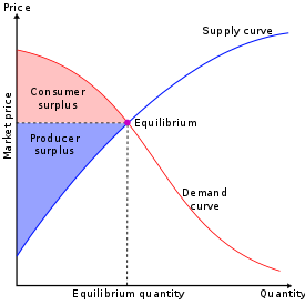
Graph illustrating consumer (red) and producer (blue) surpluses on a supply and demand chart

In mainstream economics, economic surplus, also known as total welfare or total social welfare or Marshallian surplus (after Alfred Marshall), is either of two related quantities:

• Consumer surplus, or consumers' surplus, is the monetary gain obtained by consumers because they are able to purchase a product for a price that is less than the highest price that they would be willing to pay.
• Producer surplus, or producers' surplus, is the amount that producers benefit by selling at a market price that is higher than the least that they would be willing to sell for; this is roughly equal to profit (since producers are not normally willing to sell at a loss and are normally indifferent to selling at a break-even price).

Overview

In the mid-19th century, engineer Jules Dupuit first propounded the concept of economic surplus, but it was the economist Alfred Marshall who gave the concept its fame in the field of economics.

On a standard supply and demand diagram, consumer surplus is the area (triangular if the supply and demand curves are linear) above the equilibrium price of the good and below the demand curve. This reflects the fact that consumers would have been willing to buy a single unit of the good at a price higher than the equilibrium price, a second unit at a price below that but still above the equilibrium price, etc., yet they in fact pay just the equilibrium price for each unit they buy.

Likewise, in the supply-demand diagram, producer surplus is the area below the equilibrium price but above the supply curve. This reflects the fact that producers would have been willing to supply the first unit at a price lower than the equilibrium price, the second unit at a price above that but still below the equilibrium price, etc., yet they in fact receive the equilibrium price for all the units they sell.

History

Early writers of economic issues used surplus as a means to draw conclusions about the relationship between production and necessities. In the agricultural sector surplus was an important concept because this sector has the responsibility to feed everyone plus itself. Food is notable because people only need a specific amount of food and can only consume a limited amount. This means that excess food production must overflow to other people, and will not be rationally hoarded. The non-agricultural sector is therefore limited by the agricultural sector equaling the output of food subtracting the amount consumed by the agricultural sector.

William Petty

William Petty  used a broad definition of necessities, leading him to focus on employment issues surrounding surplus. Petty explains a hypothetical example in which there is a territory of 1000 men and 100 of those men are capable of producing enough food for all 1000 men. The question becomes, what will the rest of the men do if only 100 are needed to provide necessities? He thereby suggests a variety of employments with some remaining unemployed.

David Hume

David Hume approached the agricultural surplus concept from another direction. Hume recognized that agriculture may feed more than those who cultivate it, but questioned why farmers would work to produce more than they need. Forceful production, which may occur under a feudal system, would be unlikely to generate a notable surplus in his opinion. Yet, if they could purchase luxuries and other goods beyond their necessities, they would become incentivized to produce and sell a surplus. Hume did not see this concept as abstract theory, he stated it as a fact when discussing how England developed after the introduction of foreign luxuries in his History of England.

Adam Smith

Adam Smith's thoughts on surplus drew on Hume. Smith noted that the desire for luxuries is infinite compared to the finite capacity of hunger. Smith saw the development in Europe as originating from landlords placing more importance on luxury spending rather than political power.

Consumer surplus

Consumer surplus is the difference between the maximum price a consumer is willing to pay and the actual price they do pay. If a consumer is willing to pay more for a unit of a good than the current asking price, they are getting more benefit from the purchased product than they would if the price was their maximum willingness to pay. They are receiving the same benefit, the obtainment of the good, at a lesser cost. An example of a good with generally high consumer surplus is drinking water. People would pay very high prices for drinking water, as they need it to survive. The difference in the price that they would pay, if they had to, and the amount that they pay now is their consumer surplus. The utility of the first few liters of drinking water is very high (as it prevents death), so the first few liters would likely have more consumer surplus than subsequent quantities.

The maximum amount a consumer would be willing to pay for a given quantity of a good is the sum of the maximum price they would pay for the first unit, the (lower) maximum price they would be willing to pay for the second unit, etc. Typically these prices are decreasing; they are given by the individual demand curve, which must be generated by a rational consumer who maximizes utility subject to a budget constraint. Because the demand curve is downward sloping, there is diminishing marginal utility. Diminishing marginal utility means a person receives less additional utility from an additional unit. However, the price of a product is constant for every unit at the equilibrium price. The extra money someone would be willing to pay for the number units of a product less than the equilibrium quantity and at a higher price than the equilibrium price for each of these quantities is the benefit they receive from purchasing these quantities. For a given price the consumer buys the amount for which the consumer surplus is highest. The consumer's surplus is highest at the largest number of units for which, even for the last unit, the maximum willingness to pay is not below the market price.

Consumer surplus can be used as a measurement of social welfare, shown by Robert Willig. For a single price change, consumer surplus can provide an approximation of changes in welfare. With multiple price and/or income changes, however, consumer surplus cannot be used to approximate economic welfare because it is not single-valued anymore. More modern methods are developed later to estimate the welfare effect of price changes using consumer surplus.

The aggregate consumers' surplus is the sum of the consumer's surplus for all individual consumers. This aggregation can be represented graphically, as shown in the above graph of the market demand and supply curves. The aggregate consumers' surplus can also be said to be the maxim of satisfaction a consumer derives from particular goods and services.

Calculation from supply and demand

The consumer surplus (individual or aggregated) is the area under the (individual or aggregated) demand curve and above a horizontal line at the actual price (in the aggregated case, the equilibrium price). If the demand curve is a straight line, the consumer surplus is the area of a triangle:

${\displaystyle CS=\frac{1}{2}{Q}_{\mathrm{m}\mathrm{k}\mathrm{t}}\left(P_{max}-P_{\mathrm{m}\mathrm{k}\mathrm{t}}\right),}$

where P_mkt is the equilibrium price (where supply equals demand), Q_mkt is the total quantity purchased at the equilibrium price, and P_max is the price at which the quantity purchased would fall to 0 (that is, where the demand curve intercepts the price axis). For more general demand and supply functions, these areas are not triangles but can still be found using integral calculus. Consumer surplus is thus the definite integral of the demand function with respect to price, from the market price to the maximum reservation price (i.e., the price-intercept of the demand function):

${\displaystyle CS={\int }_{P_{\mathrm{m}\mathrm{k}\mathrm{t}}}^{P_{max}}D(P)dP,}$

where ${\displaystyle D(P_{max})=0.}$ This shows that if we see a rise in the equilibrium price and a fall in the equilibrium quantity, then consumer surplus falls.

Calculation of a change in consumer surplus

The change in consumer surplus is used to measure the changes in prices and income. The demand function used to represent an individual's demand for a certain product is essential in determining the effects of a price change. An individual's demand function is a function of the individual's income, the demographic characteristics of the individual, and the vector of commodity prices. When the price of a product changes, the change in consumer surplus is measured as the negative value of the integral from the original actual price (P₀) and the new actual price (P₁) of the demand for product by the individual. If the change in consumer surplus is positive, the price change is said to have increased the individuals welfare. If the price change in consumer surplus is negative, the price change is said to have decreased the individual's welfare.

Distribution of benefits when price falls

When supply of a good expands, the price falls (assuming the demand curve is downward sloping) and consumer surplus increases. This benefits two groups of people: consumers who were already willing to buy at the initial price benefit from a price reduction, and they may buy more and receive even more consumer surplus; and additional consumers who were unwilling to buy at the initial price will buy at the new price and also receive some consumer surplus.

Consider an example of linear supply and demand curves. For an initial supply curve S₀, consumer surplus is the triangle above the line formed by price P₀ to the demand line (bounded on the left by the price axis and on the top by the demand line). If supply expands from S₀ to S₁, the consumers' surplus expands to the triangle above P₁ and below the demand line (still bounded by the price axis). The change in consumer's surplus is difference in area between the two triangles, and that is the consumer welfare associated with expansion of supply.

Some people were willing to pay the higher price P₀. When the price is reduced, their benefit is the area in the rectangle formed on the top by P₀, on the bottom by P₁, on the left by the price axis and on the right by line extending vertically upwards from Q₀.

The second set of beneficiaries are consumers who buy more, and new consumers, those who will pay the new lower price (P₁) but not the higher price (P₀). Their additional consumption makes up the difference between Q₁ and Q₀. Their consumer surplus is the triangle bounded on the left by the line extending vertically upwards from Q₀, on the right and top by the demand line, and on the bottom by the line extending horizontally to the right from P₁.

Rule of one-half

The rule of one-half estimates the change in consumer surplus for small changes in supply with a constant demand curve. Note that in the special case where the consumer demand curve is linear, consumer surplus is the area of the triangle bounded by the vertical line Q = 0, the horizontal line ${\displaystyle P=P_{\mathrm{m}\mathrm{k}\mathrm{t}}}$ and the linear demand curve. Hence, the change in consumer surplus is the area of the trapezoid with i) height equal to the change in price and ii) mid-segment length equal to the average of the ex-post and ex-ante equilibrium quantities. Following the figure above,

${\displaystyle \mathrm{\Delta }CS=\frac{1}{2}(Q_1+Q_0)(P_0-P_1),}$

where:

• CS = consumers' surplus;
• Q₀ and Q₁ are, respectively, the quantity demanded before and after a change in supply;
• P₀ and P₁ are, respectively, the prices before and after a change in supply.

Producer surplus

Producer surplus is the additional benefit that the owners of production factors and product providers bring to producers due to the differences between production, the supply price of the product, and the current market price. The difference between the amount actually obtained in a market transaction and the minimum amount it is willing to accept with the production factors or the products provided.

Calculation of producer surplus

Producer surplus is usually expressed by the area below the market price line and above the supply curve. In Figure 1, the shaded areas below the price line and above the supply curve between production zero and maximum output Q₁ indicate producer surplus. Among them, OP₁EQ₁ below the price line. This indicates that the total revenue is the minimum total payment actually accepted by the manufacturer. The area OP_MEQ₁ below the S curve is the minimum total revenue that the manufacturer is willing to accept. In Figure 1, the area enclosed by the market price line, the manufacturer's supply line, and the coordinate axis is the producer surplus. Because the rectangle OP₁EQ₁ is the total revenue actually obtained by the manufacturer, that is, A + B, and the trapezoid OP_MEQ. The minimum total profit that the manufacturer is willing to accept, that is, B, so A is the producer surplus.

Producer surplus

Obviously, the manufacturer produces and sells a certain quantity of Q₁ goods at the market price P₁. The manufacturer has reduced the quantity of goods for Q₁, which means that the manufacturer has increased the production factors or production costs equivalent to the amount of AVC·Q₁. However, at the same time, the manufacturer actually obtains a total income equivalent to the total market price P₁·Q₁. Since AVC is always smaller than P₁, from the production and sales of goods in Q₁, manufacturers not only get sales revenue equivalent to variable costs, but also get additional revenue. This part of the excess income reflects the increase in the benefits obtained by the manufacturers through market exchange. Therefore, in economics, producer surplus is usually used to measure producer welfare and is an important part of social welfare.

Producer surplus is usually used to measure the economic welfare obtained by the manufacturer in the market supply. When the supply price is constant, the producer welfare depends on the market price. If the manufacturer can sell the product at the highest price, the welfare is the greatest. As part of social welfare, the size of the producer surplus depends on many factors. Generally speaking, when other factors remain constant, an increase in market price will increase producer surplus, and a decrease in supply price or marginal cost will also increase producer surplus. If there is a surplus of goods, that is, people can only sell part of the goods at market prices, and producer surplus will decrease.

Obviously, the sum of the producer surplus of all manufacturers in the market constitutes the producer surplus of the entire market. Graphically, it should be expressed as the area enclosed by the market supply curve, the market price line and the coordinate axis.

Supply and demand

From Wikipedia, the free encyclopedia
https://en.wikipedia.org/wiki/Supply_and_demand

Figure 1: The price P of a product is determined by a balance between production at each price (supply S) and the desires of those with purchasing power at each price (demand D). The diagram shows a positive shift in demand from D₁ to D₂, resulting in an increase in price (P) and quantity sold (Q) of the product.

 

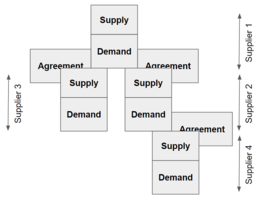
Supply and demand stacked in a conceptual chain.

In microeconomics, supply and demand is an economic model of price determination in a market. It postulates that, holding all else equal, in a competitive market, the unit price for a particular good, or other traded item such as labor or liquid financial assets, will vary until it settles at a point where the quantity demanded (at the current price) will equal the quantity supplied (at the current price), resulting in an economic equilibrium for price and quantity transacted. It forms the theoretical basis of modern economics.

In macroeconomics, as well, the aggregate demand-aggregate supply model has been used to depict how the quantity of total output and the aggregate price level may be determined in equilibrium.

Graphical representations

Supply schedule

A supply schedule, depicted graphically as a supply curve, is a table that shows the relationship between the price of a good and the quantity supplied by producers. Under the assumption of perfect competition, supply is determined by marginal cost: firms will produce additional output as long as the cost of producing an extra unit is less than the market price they receive.

A rise in the cost of raw materials would decrease supply, shifting the supply curve to the left because at each possible price a smaller quantity would be supplied. One may also think of this as a shift up in the supply curve, because the price must rise for producers to supply a given quantity. A fall in production costs would increase supply, shifting the supply curve to the right and down.

Mathematically, a supply curve is represented by a supply function, giving the quantity supplied as a function of its price and as many other variables as desired to better explain quantity supplied. The two most common specifications are:

1) linear supply function, e.g., the slanted line

${\displaystyle Q(P)=3P-6}$, and

2) the constant-elasticity supply function (also called isoelastic or log-log or loglinear supply function), e.g., the smooth curve

${\displaystyle Q(P)=5P^{0.5}}$

which can be rewritten as

${\displaystyle \log Q(P)=\log 5+0.5\log P}$

By its very nature, the concept of a supply curve assumes that firms are perfect competitors, having no influence over the market price. This is because each point on the supply curve answers the question, "If this firm is faced with this potential price, how much output will it sell?" If a firm has market power—in violation of the perfect competitor model—its decision on how much output to bring to market influences the market price. Thus the firm is not "faced with" any given price, and a more complicated model, e.g., a monopoly or oligopoly or differentiated-product model, should be used.

Economists distinguish between the supply curve of an individual firm and the market supply curve. The market supply curve shows the total quantity supplied by all firms, so it is the sum of the quantities supplied by all suppliers at each potential price (that is, the individual firms' supply curves are added horizontally).

Economists distinguish between short-run and long-run supply curve. Short run refers to a time period during which one or more inputs are fixed (typically physical capital), and the number of firms in the industry is also fixed (if it is a market supply curve). Long run refers to a time period during which new firms enter or existing firms exit and all inputs can be adjusted fully to any price change. Long-run supply curves are flatter than short-run counterparts (with quantity more sensitive to price, more elastic supply).

Common determinants of supply are:

1. Prices of inputs, including wages
2. The technology used, Productivity
3. Firms' expectations about future prices
4. Number of suppliers (for a market supply curve)

Demand schedule

A demand schedule, depicted graphically as a demand curve, represents the amount of a certain good that buyers are willing and able to purchase at various prices, assuming all other determinants of demand are held constant, such as income, tastes and preferences, and the prices of substitute and complementary goods. According to the law of demand, the demand curve is always downward-sloping, meaning that as the price decreases, consumers will buy more of the good.

Mathematically, a demand curve is represented by a demand function, giving the quantity demanded as a function of its price and as many other variables as desired to better explain quantity demanded. The two most common specifications are linear demand, e.g., the slanted line

${\displaystyle Q(P)=32-2P}$

and the constant-elasticity demand function (also called isoelastic or log-log or loglinear demand function), e.g., the smooth curve

${\displaystyle Q(P)=3P^{-2}}$

which can be rewritten as

${\displaystyle \log Q(P)=\log 3-2\log P}$

Note that really a demand curve should be drawn with price on the horizontal x-axis, since it is the independent variable. Instead, price is put on the vertical, f(x) y-axis as a matter of unfortunate historical convention.

Just as the supply curve parallels the marginal cost curve, the demand curve parallels marginal utility, measured in dollars. Consumers will be willing to buy a given quantity of a good, at a given price, if the marginal utility of additional consumption is equal to the opportunity cost determined by the price, that is, the marginal utility of alternative consumption choices. The demand schedule is defined as the willingness and ability of a consumer to purchase a given product at a certain time.

The demand curve is generally downward-sloping, but for some goods it is upward-sloping. Two such types of goods have been given definitions and names that are in common use: Veblen goods, goods which because of fashion or signalling are more attractive at higher prices, and Giffen goods, which, by virtue of being inferior goods that absorb a large part of a consumer's income (e.g., staples such as the classic example of potatoes in Ireland), may see an increase in quantity demanded when the price rises. The reason the law of demand is violated for Giffen goods is that the rise in the price of the good has a strong income effect, sharply reducing the purchasing power of the consumer so that he switches away from luxury goods to the Giffen good, e.g., when the price of potatoes rises, the Irish peasant can no longer afford meat and eats more potatoes to cover for the lost calories.

As with the supply curve, by its very nature the concept of a demand curve requires that the purchaser be a perfect competitor—that is, that the purchaser have no influence over the market price. This is true because each point on the demand curve answers the question, "If buyers are faced with this potential price, how much of the product will they purchase?" But, if a buyer has market power (that is, the amount he buys influences the price), he is not "faced with" any given price, and we must use a more complicated model, of monopsony.

As with supply curves, economists distinguish between the demand curve for an individual and the demand curve for a market. The market demand curve is obtained by adding the quantities from the individual demand curves at each price.

Common determinants of demand are:

1. Income
2. Tastes and preferences
3. Prices of related goods and services
4. Consumers' expectations about future prices and incomes
5. Number of potential consumers
6. Advertising

History of the curves

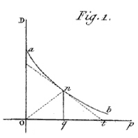
Cournot’s Recherches (1838)

 

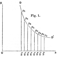
Jenkin’s Graphical Representation (1870)

 

Marshall’s Principles (1890)

Figure 2. Early supply and demand curves

Since supply and demand can be considered as functions of price they have a natural graphical representation. Demand curves were first drawn by Augustin Cournot in his Recherches sur les Principes Mathématiques de la Théorie des Richesses (1838) – see Cournot competition. Supply curves were added by Fleeming Jenkin in The Graphical Representation of the Laws of Supply and Demand... of 1870. Both sorts of curve were popularised by Alfred Marshall who, in his Principles of Economics (1890), chose to represent price – normally the independent variable – by the vertical axis; a practice which remains common.

If supply or demand is a function of other variables besides price, it may be represented by a family of curves (with a change in the other variables constituting a shift between curves) or by a surface in a higher dimensional space.

Microeconomics

Figure 3: Supply and Demand

Equilibrium

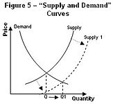
Generally speaking, an equilibrium is defined to be the price-quantity pair where the quantity demanded is equal to the quantity supplied. It is represented by the intersection of the demand and supply curves. The analysis of various equilibria is a fundamental aspect of microeconomics:

Market equilibrium: A situation in a market when the price is such that the quantity demanded by consumers is correctly balanced by the quantity that firms wish to supply. In this situation, the market clears.

Changes in market equilibrium: Practical uses of supply and demand analysis often center on the different variables that change equilibrium price and quantity, represented as shifts in the respective curves. Comparative statics of such a shift traces the effects from the initial equilibrium to the new equilibrium.

Demand curve shifts:

Main article: Demand curve

When consumers increase the quantity demanded at a given price, it is referred to as an increase in demand. Increased demand can be represented on the graph as the curve being shifted to the right. At each price point, a greater quantity is demanded, as from the initial curve D₁ to the new curve D₂. In the diagram, this raises the equilibrium price from P₁ to the higher P₂. This raises the equilibrium quantity from Q₁ to the higher Q₂. (A movement along the curve is described as a "change in the quantity demanded" to distinguish it from a "change in demand," that is, a shift of the curve.) The increase in demand has caused an increase in (equilibrium) quantity. The increase in demand could come from changing tastes and fashions, incomes, price changes in complementary and substitute goods, market expectations, and number of buyers. This would cause the entire demand curve to shift changing the equilibrium price and quantity. Note in the diagram that the shift of the demand curve, by causing a new equilibrium price to emerge, resulted in movement along the supply curve from the point (Q₁, P₁) to the point (Q₂, P₂).

If the demand decreases, then the opposite happens: a shift of the curve to the left. If the demand starts at D₂, and decreases to D₁, the equilibrium price will decrease, and the equilibrium quantity will also decrease. The quantity supplied at each price is the same as before the demand shift, reflecting the fact that the supply curve has not shifted; but the equilibrium quantity and price are different as a result of the change (shift) in demand.

Supply curve shifts:

Main article: Supply (economics)

When technological progress occurs, the supply curve shifts. For example, assume that someone invents a better way of growing wheat so that the cost of growing a given quantity of wheat decreases. Otherwise stated, producers will be willing to supply more wheat at every price and this shifts the supply curve S₁ outward, to S₂—an increase in supply. This increase in supply causes the equilibrium price to decrease from P₁ to P₂. The equilibrium quantity increases from Q₁ to Q₂ as consumers move along the demand curve to the new lower price. As a result of a supply curve shift, the price and the quantity move in opposite directions. If the quantity supplied decreases, the opposite happens. If the supply curve starts at S₂, and shifts leftward to S₁, the equilibrium price will increase and the equilibrium quantity will decrease as consumers move along the demand curve to the new higher price and associated lower quantity demanded. The quantity demanded at each price is the same as before the supply shift, reflecting the fact that the demand curve has not shifted. But due to the change (shift) in supply, the equilibrium quantity and price have changed.

The movement of the supply curve in response to a change in a non-price determinant of supply is caused by a change in the y-intercept, the constant term of the supply equation. The supply curve shifts up and down the y axis as non-price determinants of demand change.

Partial equilibrium

Main article: Partial equilibrium

Partial equilibrium, as the name suggests, takes into consideration only a part of the market to attain equilibrium.

Jain proposes (attributed to George Stigler): "A partial equilibrium is one which is based on only a restricted range of data, a standard example is price of a single product, the prices of all other products being held fixed during the analysis."

The supply-and-demand model is a partial equilibrium model of economic equilibrium, where the clearance on the market of some specific goods is obtained independently from prices and quantities in other markets. In other words, the prices of all substitutes and complements, as well as income levels of consumers are constant. This makes analysis much simpler than in a general equilibrium model which includes an entire economy.

Here the dynamic process is that prices adjust until supply equals demand. It is a powerfully simple technique that allows one to study equilibrium, efficiency and comparative statics. The stringency of the simplifying assumptions inherent in this approach makes the model considerably more tractable, but may produce results which, while seemingly precise, do not effectively model real world economic phenomena.

Partial equilibrium analysis examines the effects of policy action in creating equilibrium only in that particular sector or market which is directly affected, ignoring its effect in any other market or industry assuming that they being small will have little impact if any.

Hence this analysis is considered to be useful in constricted markets.

Léon Walras first formalized the idea of a one-period economic equilibrium of the general economic system, but it was French economist Antoine Augustin Cournot and English political economist Alfred Marshall who developed tractable models to analyze an economic system.

Other markets

The model of supply and demand also applies to various specialty markets.

The model is commonly applied to wages, in the market for labor. The typical roles of supplier and demander are reversed. The suppliers are individuals, who try to sell their labor for the highest price. The demanders of labor are businesses, which try to buy the type of labor they need at the lowest price. The equilibrium price for a certain type of labor is the wage rate. However, economist Steve Fleetwood revisited the empirical reality of supply and demand curves in labor markets and concluded that the evidence is "at best inconclusive and at worst casts doubt on their existence." For instance, he cites Kaufman and Hotchkiss (2006): "For adult men, nearly all studies find the labour supply curve to be negatively sloped or backward bending."

In both classical and Keynesian economics, the money market is analyzed as a supply-and-demand system with interest rates being the price. The money supply may be a vertical supply curve, if the central bank of a country chooses to use monetary policy to fix its value regardless of the interest rate; in this case the money supply is totally inelastic. On the other hand, the money supply curve is a horizontal line if the central bank is targeting a fixed interest rate and ignoring the value of the money supply; in this case the money supply curve is perfectly elastic. The demand for money intersects with the money supply to determine the interest rate.

According to some studies, the laws of supply and demand are applicable not only to the business relationships of people, but to the behaviour of social animals and to all living things that interact on the biological markets in scarce resource environments.

The model of supply and demand accurately describes the characteristic of metabolic systems: specifically, it explains how feedback inhibition allows metabolic pathways to respond to the demand for a metabolic intermediates while minimizing effects due to variation in the supply.

Empirical estimation

Demand and supply relations in a market can be statistically estimated from price, quantity, and other data with sufficient information in the model. This can be done with simultaneous-equation methods of estimation in econometrics. Such methods allow solving for the model-relevant "structural coefficients," the estimated algebraic counterparts of the theory. The Parameter identification problem is a common issue in "structural estimation." Typically, data on exogenous variables (that is, variables other than price and quantity, both of which are endogenous variables) are needed to perform such an estimation. An alternative to "structural estimation" is reduced-form estimation, which regresses each of the endogenous variables on the respective exogenous variables.

Macroeconomic uses

Demand and supply have also been generalized to explain macroeconomic variables in a market economy, including the quantity of total output and the aggregate price level. The aggregate demand-aggregate supply model may be the most direct application of supply and demand to macroeconomics, but other macroeconomic models also use supply and demand. Compared to microeconomic uses of demand and supply, different (and more controversial) theoretical considerations apply to such macroeconomic counterparts as aggregate demand and aggregate supply. Demand and supply are also used in macroeconomic theory to relate money supply and money demand to interest rates, and to relate labor supply and labor demand to wage rates.

History

The 256th couplet of Tirukkural, which was composed at least 2000 years ago, says that "if people do not consume a product or service, then there will not be anybody to supply that product or service for the sake of price".

According to Hamid S. Hosseini, the power of supply and demand was understood to some extent by several early Muslim scholars, such as fourteenth-century Syrian scholar Ibn Taymiyyah, who wrote: "If desire for goods increases while its availability decreases, its price rises. On the other hand, if availability of the good increases and the desire for it decreases, the price comes down."

If desire for goods increases while its availability decreases, its price rises. On the other hand, if availability of the good increases and the desire for it decreases, the price comes down.

— Ibn Taymiyyah, 

Adam Smith

Shifting focus to the English etymology of the expression, it has been confirmed that the phrase 'supply and demand' was not used by English economics writers until after the end of the 17th century. In John Locke's 1691 work Some Considerations on the Consequences of the Lowering of Interest and the Raising of the Value of Money, Locke alluded to the idea of supply and demand, however, he failed to accurately label it as such and thus, he fell short in coining the phrase and conveying its true significance. Locke wrote: “The price of any commodity rises or falls by the proportion of the number of buyer and sellers” and “that which regulates the price... [of goods] is nothing else but their quantity in proportion to [the] Vent.” Locke's terminology drew criticism from John Law. Law argued that,"The Prices of Goods are not according to the quantity in proportion to the Vent, but in proportion to the Demand." From Law the demand part of the phrase was given its proper title and it began to circulate among "prominent authorities" in the 1730s. In 1755, Francis Hutcheson, in his A System of Moral Philosophy, furthered development toward the phrase by stipulating that, "the prices of goods depend on these two jointly, the Demand... and the Difficulty of acquiring."

It was not until 1767 that the phrase "supply and demand" was first used by Scottish writer James Denham-Steuart in his Inquiry into the Principles of Political Economy. He originated the use of this phrase by effectively combining "supply" and "demand" together in a number of different occasions such as price determination and competitive analysis. In Steuart's chapter entitled "Of Demand", he argues that "The nature of Demand is to encourage industry; and when it is regularly made, the effect of it is, that the supply for the most part is found to be in proportion to it, and then the demand is simple". It is presumably from this chapter that the idea spread to other authors and economic thinkers. Adam Smith used the phrase after Steuart in his 1776 book The Wealth of Nations. In The Wealth of Nations, Smith asserted that the supply price was fixed but that its "merit" (value) would decrease as its "scarcity" increased, this idea by Smith was later named the law of demand. In 1803, Thomas Robert Malthus used the phrase "supply and demand" twenty times in the second edition of the Essay on Population. And David Ricardo in his 1817 work, Principles of Political Economy and Taxation, titled one chapter, "On the Influence of Demand and Supply on Price". In Principles of Political Economy and Taxation, Ricardo more rigorously laid down the idea of the assumptions that were used to build his ideas of supply and demand. In 1838, Antoine Augustin Cournot developed a mathematical model of supply and demand in his Researches into the Mathematical Principles of Wealth, it included diagrams. It is important to note that the use of the phrase was still rare and only a few examples of more than 20 uses in a single work have been identified by the end of the second decade of the 19th century.

During the late 19th century the marginalist school of thought emerged. The main innovators of this approach were Stanley Jevons, Carl Menger, and Léon Walras. The key idea was that the price was set by the subjective value of a good at the margin. This was a substantial change from Adam Smith's thoughts on determining the supply price.

In his 1870 essay "On the Graphical Representation of Supply and Demand", Fleeming Jenkin in the course of "introduc[ing] the diagrammatic method into the English economic literature" published the first drawing of supply and demand curves in English, including comparative statics from a shift of supply or demand and application to the labor market. The model was further developed and popularized by Alfred Marshall in the 1890 textbook Principles of Economics.

Criticism

The philosopher Hans Albert has argued that the ceteris paribus conditions of the marginalist theory rendered the theory itself an empty tautology and completely closed to experimental testing. In essence, he argues, the supply and demand curves (theoretical functions which express the quantity of a product which would be offered or requested for a given price) are purely ontological.

Piero Sraffa's critique focused on the inconsistency (except in implausible circumstances) of partial equilibrium analysis and the rationale for the upward slope of the supply curve in a market for a produced consumption good. The notability of Sraffa's critique is also demonstrated by Paul Samuelson's comments and engagements with it over many years, for example:

What a cleaned-up version of Sraffa (1926) establishes is how nearly empty are all of Marshall's partial equilibrium boxes. To a logical purist of Wittgenstein and Sraffa class, the Marshallian partial equilibrium box of constant cost is even more empty than the box of increasing cost.

Modern Post-Keynesians criticize the supply and demand model for failing to explain the prevalence of administered prices, in which retail prices are set by firms, primarily based on a mark-up over normal average unit costs, and aren't responsive to changes in demand up to capacity.

Some economists criticize the conventional supply and demand theory for failing to explain or anticipate asset bubbles that can arise from a positive feedback loop. Conventional supply and demand theory assumes that expectations of consumers do not change as a consequence of price changes. In scenarios such as the United States housing bubble, an initial price change of an asset can increase the expectations of investors, making the asset more lucrative and contributing to further price increases until market sentiment changes, which creates a positive feedback loop and an asset bubble. Asset bubbles cannot be understood in the conventional supply and demand framework because the conventional system assumes a price change will be self-correcting and the system will snap back to equilibrium.

Paul Cockshott's critique focuses on the unfalsifiability of the neoclassical model. In the linear examples given above we have four unknowns: the slope and intercept of both the supply curve and the demand curve. But because we only have two knowns, price and quantity, any set of supply and demand curves that crosses the point ${\displaystyle (Q,P)}$ could explain the data. Hence unfalsifiability. Cockshott also points out that prices are negatively correlated with quantity due to economies of scale, not positively correlated as the theory suggests. Finally, Cockshott argues that the theory is needlessly complicated when compared to the labour theory of value, and that having to introduce a notion of the curves shifting amounts to adding epicycles.