Search This Blog

Friday, August 18, 2023

Swamp

From Wikipedia, the free encyclopedia
https://en.wikipedia.org/wiki/Swamp

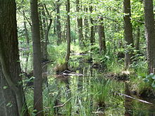
A freshwater swamp in Florida, United States

A swamp is a forested wetland. Swamps are considered to be transition zones because both land and water play a role in creating this environment. Swamps vary in size and are located all around the world. The water of a swamp may be fresh water, brackish water, or seawater. Freshwater swamps form along large rivers or lakes where they are critically dependent upon rainwater and seasonal flooding to maintain natural water level fluctuations. Saltwater swamps are found along tropical and subtropical coastlines. Some swamps have hammocks, or dry-land protrusions, covered by aquatic vegetation, or vegetation that tolerates periodic inundation or soil saturation. The two main types of swamp are "true" or swamp forests and "transitional" or shrub swamps. In the boreal regions of Canada, the word swamp is colloquially used for what is more formally termed a bog, fen, or muskeg. Some of the world's largest swamps are found along major rivers such as the Amazon, the Mississippi, and the Congo.

Differences between marshes and swamps

Difference between swamp and marsh

Swamps and marshes are specific types of wetlands that form along waterbodies containing rich, hydric soils. Marshes are wetlands, continually or frequently flooded by nearby running bodies of water, that are dominated by emergent soft-stem vegetation and herbaceous plants. Swamps are wetlands consisting of saturated soils or standing water and are dominated by water-tolerant woody vegetation such as shrubs, bushes, and trees.

Hydrology

Swamps are characterized by their saturated soils and slow-moving waters. The water that accumulates in swamps comes from a variety of sources including precipitation, groundwater, tides and/or freshwater flooding. These hydrologic pathways all contribute to how energy and nutrients flow in and out of the ecosystem. As water flows through the swamp, nutrients, sediment and pollutants are naturally filtered out. Chemicals like phosphorus and nitrogen that end up in waterways get absorbed and used by the aquatic plants within the swamp, purifying the water. Any remaining or excess chemicals present will accumulate at the bottom of the swamp, being removed from the water and buried within the sediment. The biogeochemical environment of a swamp is dependent on its hydrology, affecting the levels and availability of resources like oxygen, nutrients, water pH and toxicity, which will influence the whole ecosystem.

Values and ecosystem services

The Linnaistensuo Mire, a nature reserve swamp in Lahti, Finland.

Swamps and other wetlands have traditionally held a very low property value compared to fields, prairies, or woodlands. They have a reputation for being unproductive land that cannot easily be utilized for human activities, other than hunting, trapping, or fishing. Farmers, for example, typically drained swamps next to their fields so as to gain more land usable for planting crops, both historically, and to a lesser extent, presently. On the other hand, swamps can (and do) play a beneficial ecological role in the overall functions of the natural environment and provide a variety of resources that many species depend on. Swamps and other wetlands have shown to be a natural form of flood management and defense against flooding. In such circumstances where flooding does occur, swamps absorb and use the excess water within the wetland, preventing it from traveling and flooding surrounding areas. Dense vegetation within the swamp also provides soil stability to the land, holding soils and sediment in place whilst preventing erosion and land loss. Swamps are an abundant and valuable source of fresh water and oxygen for all life, and they are often breeding grounds for a wide variety of species. Floodplain swamps are an important resource in the production and distribution of fish. Two thirds of global fish and shellfish are commercially harvested and dependent on wetlands.

Impacts and conservation

Historically, humans have been known to drain and/or fill swamps and other wetlands in order to create more space for human development and to reduce the threat of diseases borne by swamp insects. Wetlands are removed and replaced with land that is then used for things like agriculture, real estate, and recreational uses. Many swamps have also undergone intensive logging and farming, requiring the construction of drainage ditches and canals. These ditches and canals contributed to drainage and, along the coast, allowed salt water to intrude, converting swamps to marsh or even to open water. Large areas of swamp were therefore lost or degraded. Louisiana provides a classic example of wetland loss from these combined factors. Europe has probably lost nearly half its wetlands. New Zealand lost 90 percent of its wetlands over a period of 150 years. Ecologists recognize that swamps provide ecological services including flood control, fish production, water purification, carbon storage, and wildlife habitats. In many parts of the world authorities protect swamps. In parts of Europe and North America, swamp restoration projects are becoming widespread. The United States government began enforcing stricter laws and management programs in the 1970s in efforts to protect and restore these ecosystems. Often the simplest steps to restoring swamps involve plugging drainage ditches and removing levees.

Conservationists work to preserve swamps such as those in northwest Indiana in the United States Midwest that were preserved as part of the Indiana Dunes.

Notable examples

Swamps can be found on all continents except Antarctica.

The largest swamp in the world is the Amazon River floodplain, which is particularly significant for its large number of fish and tree species.

Africa

The Sudd and the Okavango Delta are Africa's best known marshland areas. The Bangweulu Floodplains make up Africa's largest swamp.

Asia

Marsh Arabs poling a mashoof

The Mesopotamian Marshes is a large swamp and river system in southern Iraq, traditionally inhabited in part by the Marsh Arabs.

In Asia, tropical peat swamps are located in mainland East Asia and Southeast Asia. In Southeast Asia, peatlands are mainly found in low altitude coastal and sub-coastal areas and extend inland for distance more than 100 km (62 mi) along river valleys and across watersheds. They are mostly to be found on the coasts of East Sumatra, Kalimantan (Central, East, South and West Kalimantan provinces), West Papua, Papua New Guinea, Brunei, Peninsular Malaya, Sabah, Sarawak, Southeast Thailand, and the Philippines (Riley et al.,1996). Indonesia has the largest area of tropical peatland. Of the total 440,000 km2 (170,000 sq mi) tropical peat swamp, about 210,000 km2 (81,000 sq mi) are located in Indonesia (Page, 2001; Wahyunto, 2006).

The Vasyugan Swamp is a large swamp in the western Siberia area of the Russian Federation. This is one of the largest swamps in the world, covering an area larger than Switzerland.

North America
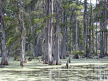
Swamp in southern Louisiana

The Atchafalaya Swamp at the lower end of the Mississippi River is the largest swamp in the United States. It is an important example of southern cypress swamp but it has been greatly altered by logging, drainage and levee construction. Other famous swamps in the United States are the forested portions of the Everglades, Okefenokee Swamp, Barley Barber Swamp, Great Cypress Swamp and the Great Dismal Swamp. The Okefenokee is located in extreme southeastern Georgia and extends slightly into northeastern Florida. The Great Cypress Swamp is mostly in Delaware but extends into Maryland on the Delmarva Peninsula. Point Lookout State Park on the southern tip of Maryland contains a large amount of swamps and marshes. The Great Dismal Swamp lies in extreme southeastern Virginia and extreme northeastern North Carolina. Both are National Wildlife Refuges. Another swamp area, Reelfoot Lake of extreme western Tennessee and Kentucky, was created by the 1811–12 New Madrid earthquakes. Caddo Lake, the Great Dismal and Reelfoot are swamps that are centered at large lakes. Swamps are often associated with bayous in the southeastern United States, especially in the Gulf Coast region. A baygall is a type of swamp found in the forest of the Gulf Coast states in the USA.

List of major swamps

A small swamp in Padstow, New South Wales, Australia
Inside a mangrove canopy, Salt Pan Creek, New South Wales

The world's largest wetlands include significant areas of swamp, such as in the Amazon and Congo River basins. Further north, however, the largest wetlands are bogs.

Africa

Asia

Australia

Europe

A black alder swamp in Germany

North America

South America

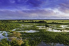
Pantanal in Brazil

Sex-determination system

From Wikipedia, the free encyclopedia
https://en.wikipedia.org/wiki/Sex-determination_system

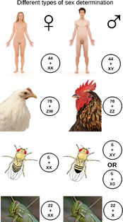
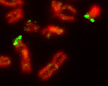
Some chromosomal sex determination systems in animals

A sex-determination system is a biological system that determines the development of sexual characteristics in an organism. Most organisms that create their offspring using sexual reproduction have two common sexes and a few less common intersex variations.

In some species there are hermaphrodites. There are also some species that are only one sex due to parthenogenesis, the act of a female reproducing without fertilization.

In some species, sex determination is genetic: males and females have different alleles or even different genes that specify their sexual morphology. In animals this is often accompanied by chromosomal differences, generally through combinations of XY, ZW, XO, ZO chromosomes, or haplodiploidy. The sexual differentiation is generally triggered by a main gene (a "sex locus"), with a multitude of other genes following in a domino effect.

In other cases, sex of a fetus is determined by environmental variables (such as temperature). The details of some sex-determination systems are not yet fully understood. Hopes for future fetal biological system analysis include complete-reproduction-system initialized signals that can be measured during pregnancies to more accurately determine whether a determined sex of a fetus is male, or female. Such analysis of biological systems could also signal whether the fetus is hermaphrodite, which includes total or partial of both male and female reproduction organs.

Some species such as various plants and fish do not have a fixed sex, and instead go through life cycles and change sex based on genetic cues during corresponding life stages of their type. This could be due to environmental factors such as seasons and temperature. In some gonochoric species, a few individuals may have sex characteristics of both sexes, a condition called intersex.

While diversity in sex determination systems is common throughout different biological systems, the systems beyond XY/XX/XO in mammals are often left to more advanced courses for those whose studies specialize in genetics of other organisms.

Discovery

Sex determination was discovered in the mealworm by the American geneticist Nettie Stevens in 1903.

Chromosomal systems

XX/XY sex chromosomes

Drosophila sex-chromosomes
Human male XY chromosomes after G-banding

The XX/XY sex-determination system is the most familiar, as it is found in humans. The XX/XY system is found in most other mammals, as well as some insects. In this system, most females have two of the same kind of sex chromosome (XX), while most males have two distinct sex chromosomes (XY). The X and Y sex chromosomes are different in shape and size from each other, unlike the rest of the chromosomes (autosomes), and are sometimes called allosomes. In some species, such as humans, organisms remain sex indifferent for a time after they're created; in others, however, such as fruit flies, sexual differentiation occurs as soon as the egg is fertilized.

Y-centered sex determination

Some species (including humans) have a gene SRY on the Y chromosome that determines maleness. Members of SRY-reliant species can have uncommon XY chromosomal combinations such as XXY and still live. Human sex is determined by the presence or absence of a Y chromosome with a functional SRY gene. Once the SRY gene is activated, cells create testosterone and anti-müllerian hormone which typically ensures the development of a single, male reproductive system. In typical XX embryos, cells secrete estrogen, which drives the body toward the female pathway.

In Y-centered sex determination, the SRY gene is the main gene in determining male characteristics, but multiple genes are required to develop testes. In XY mice, lack of the gene DAX1 on the X chromosome results in sterility, but in humans it causes adrenal hypoplasia congenita. However, when an extra DAX1 gene is placed on the X chromosome, the result is a female, despite the existence of SRY. Even when there are normal sex chromosomes in XX females, duplication or expression of SOX9 causes testes to develop. Gradual sex reversal in developed mice can also occur when the gene FOXL2 is removed from females. Even though the gene DMRT1 is used by birds as their sex locus, species who have XY chromosomes also rely upon DMRT1, contained on chromosome 9, for sexual differentiation at some point in their formation.

X-centered sex determination

Some species, such as fruit flies, use the presence of two X chromosomes to determine femaleness. Species that use the number of Xs to determine sex are nonviable with an extra X chromosome.

Other variants of XX/XY sex determination

Some fish have variants of the XY sex-determination system, as well as the regular system. For example, while having an XY format, Xiphophorus nezahualcoyotl and X. milleri also have a second Y chromosome, known as Y', that creates XY' females and YY' males.

At least one monotreme, the platypus, presents a particular sex determination scheme that in some ways resembles that of the ZW sex chromosomes of birds and lacks the SRY gene. The platypus has ten sex chromosomes; males have an XYXYXYXYXY pattern while females have ten X chromosomes. Although it is an XY system, the platypus' sex chromosomes share no homologues with eutherian sex chromosomes. Instead, homologues with eutherian sex chromosomes lie on the platypus chromosome 6, which means that the eutherian sex chromosomes were autosomes at the time that the monotremes diverged from the therian mammals (marsupials and eutherian mammals). However, homologues to the avian DMRT1 gene on platypus sex chromosomes X3 and X5 suggest that it is possible the sex-determining gene for the platypus is the same one that is involved in bird sex-determination. More research must be conducted in order to determine the exact sex determining gene of the platypus.

Heredity of sex chromosomes in XO sex determination

XX/X0 sex chromosomes

In this variant of the XY system, females have two copies of the sex chromosome (XX) but males have only one (X0). The 0 denotes the absence of a second sex chromosome. Generally in this method, the sex is determined by amount of genes expressed across the two chromosomes. This system is observed in a number of insects, including the grasshoppers and crickets of order Orthoptera and in cockroaches (order Blattodea). A small number of mammals also lack a Y chromosome. These include the Amami spiny rat (Tokudaia osimensis) and the Tokunoshima spiny rat (Tokudaia tokunoshimensis) and Sorex araneus, a shrew species. Transcaucasian mole voles (Ellobius lutescens) also have a form of XO determination, in which both sexes lack a second sex chromosome. The mechanism of sex determination is not yet understood.

The nematode C. elegans is male with one sex chromosome (X0); with a pair of chromosomes (XX) it is a hermaphrodite. Its main sex gene is XOL, which encodes XOL-1 and also controls the expression of the genes TRA-2 and HER-1. These genes reduce male gene activation and increase it, respectively.

ZW/ZZ sex chromosomes

The ZW sex-determination system is found in birds, some reptiles, and some insects and other organisms. The ZW sex-determination system is reversed compared to the XY system: females have two different kinds of chromosomes (ZW), and males have two of the same kind of chromosomes (ZZ). In the chicken, this was found to be dependent on the expression of DMRT1. In birds, the genes FET1 and ASW are found on the W chromosome for females, similar to how the Y chromosome contains SRY. However, not all species depend upon the W for their sex. For example, there are moths and butterflies that are ZW, but some have been found female with ZO, as well as female with ZZW. Also, while mammals deactivate one of their extra X chromosomes when female, it appears that in the case of Lepidoptera, the males produce double the normal amount of enzymes, due to having two Z's. Because the use of ZW sex determination is varied, it is still unknown how exactly most species determine their sex. However, reportedly, the silkworm Bombyx mori uses a single female-specific piRNA as the primary determiner of sex. Despite the similarities between the ZW and XY systems, these sex chromosomes evolved separately. In the case of the chicken, their Z chromosome is more similar to humans' autosome 9. The chicken's Z chromosome also seems to be related to the X chromosome of the platypus. When a ZW species, such as the Komodo dragon, reproduces parthenogenetically, usually only males are produced. This is due to the fact that the haploid eggs double their chromosomes, resulting in ZZ or WW. The ZZ become males, but the WW are not viable and are not brought to term.

In both XY and ZW sex determination systems, the sex chromosome carrying the critical factors is often significantly smaller, carrying little more than the genes necessary for triggering the development of a given sex.

ZZ/Z0 sex chromosomes

The ZZ/Z0 sex-determination system is found in some moths. In these insects there is one sex chromosome, Z. Males have two Z chromosomes, whereas females have one Z. Males are ZZ, while females are Z0.

UV sex chromosomes

In some Bryophyte and some algae species, the gametophyte stage of the life cycle, rather than being hermaphrodite, occurs as separate male or female individuals that produce male and female gametes respectively. When meiosis occurs in the sporophyte generation of the life cycle, the sex chromosomes known as U and V assort in spores that carry either the U chromosome and give rise to female gametophytes, or the V chromosome and give rise to male gametophytes.

Haplodiploid sex chromosomes

Haplodiploidy

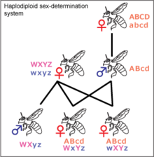
Haplodiploidy is found in insects belonging to Hymenoptera, such as ants and bees. Sex determination is controlled by the zygosity of a complementary sex determiner (csd) locus. Unfertilized eggs develop into haploid individuals which have a single, hemizygous copy of the csd locus and are therefore males. Fertilized eggs develop into diploid individuals which, due to high variability in the csd locus, are generally heterozygous females. In rare instances diploid individuals may be homozygous, these develop into sterile males. The gene acting as a csd locus has been identified in the honeybee and several candidate genes have been proposed as a csd locus for other Hymenopterans. Most females in the Hymenoptera order can decide the sex of their offspring by holding received sperm in their spermatheca and either releasing it into their oviduct or not. This allows them to create more workers, depending on the status of the colony.

Other chromosomal systems

Other uncommon systems include those of the green swordtail (a polyfactorial system with the sex-determining genes on several chromosomes) the Chironomus midges; the juvenile hermaphroditism of zebrafish, with an unknown trigger; and the platyfish, which has W, X, and Y chromosomes. This allows WY, WX, or XX females and YY or XY males.

Mating type in microorganisms is analogous to sex in multi-cellular organisms, and is sometimes described using those terms, though they are not necessarily correlated with physical body structures. Some species have more than two mating types. Tetrahymena, a type of ciliate, has seven mating types. Schizophyllum commune, a type of fungus, has 23,328.

Environmental systems

All alligators determine the sex of their offspring by the temperature of the nest.

Temperature-dependent

Many other sex-determination systems exist. In some species of reptiles, including alligators, some turtles, and the tuatara, sex is determined by the temperature at which the egg is incubated during a temperature-sensitive period. There are no examples of temperature-dependent sex determination (TSD) in birds. Megapodes had formerly been thought to exhibit this phenomenon, but were found to actually have different temperature-dependent embryo mortality rates for each sex. For some species with TSD, sex determination is achieved by exposure to hotter temperatures resulting in the offspring being one sex and cooler temperatures resulting in the other. This type of TSD is called Pattern I. For others species using TSD, it is exposure to temperatures on both extremes that results in offspring of one sex, and exposure to moderate temperatures that results in offspring of the opposite sex, called Pattern II TSD. The specific temperatures required to produce each sex are known as the female-promoting temperature and the male-promoting temperature. When the temperature stays near the threshold during the temperature sensitive period, the sex ratio is varied between the two sexes. Some species' temperature standards are based on when a particular enzyme is created. These species that rely upon temperature for their sex determination do not have the SRY gene, but have other genes such as DAX1, DMRT1, and SOX9 that are expressed or not expressed depending on the temperature. The sex of some species, such as the Nile tilapia, Australian skink lizard, and Australian dragon lizard, has an initial bias, set by chromosomes, but can later be changed by the temperature of incubation.

It is unknown how exactly temperature-dependent sex determination evolved. It could have evolved through certain sexes being more suited to certain areas that fit the temperature requirements. For example, a warmer area could be more suitable for nesting, so more females are produced to increase the amount that nest next season. In amniotes, environmental sex determination preceded the genetically determined systems of birds and mammals; it is thought that a temperature-dependent amniote was the common ancestor of amniotes with sex chromosomes.

Other environmental systems

There are other environmental sex determination systems including location-dependent determination systems as seen in the marine worm Bonellia viridis – larvae become males if they make physical contact with a female, and females if they end up on the bare sea floor. This is triggered by the presence of a chemical produced by the females, bonellin. Some species, such as some snails, practice sex change: adults start out male, then become female. In tropical clown fish, the dominant individual in a group becomes female while the other ones are male, and bluehead wrasses (Thalassoma bifasciatum) are the reverse. Some species, however, have no sex-determination system. Hermaphrodite species include the common earthworm and certain species of snails. A few species of fish, reptiles, and insects reproduce by parthenogenesis and are female altogether. There are some reptiles, such as the boa constrictor and Komodo dragon that can reproduce both sexually and asexually, depending on whether a mate is available.

Evolution

The ends of the XY chromosomes, highlighted here in green, are all that is left of the original autosomes that can still cross over with each other.

Sex determination systems may have evolved from mating type, which is a feature of microorganisms.

Chromosomal sex determination may have evolved early in the history of eukaryotes. But in plants it has been suggested to have evolved recently.

The accepted hypothesis of XY and ZW sex chromosome evolution in amniotes is that they evolved at the same time, in two different branches.

No genes are shared between the avian ZW and mammal XY chromosomes and the chicken Z chromosome is similar to the human autosomal chromosome 9, rather than X or Y. This suggests not that the ZW and XY sex-determination systems share an origin but that the sex chromosomes are derived from autosomal chromosomes of the common ancestor of birds and mammals. In the platypus, a monotreme, the X1 chromosome shares homology with therian mammals, while the X5 chromosome contains an avian sex-determination gene, further suggesting an evolutionary link.

However, there is some evidence to suggest that there could have been transitions between ZW and XY, such as in Xiphophorus maculatus, which have both ZW and XY systems in the same population, despite the fact that ZW and XY have different gene locations. A recent theoretical model raises the possibility of both transitions between the XY/XX and ZZ/ZW system and environmental sex determination. The platypus' genes also back up the possible evolutionary link between XY and ZW, because they have the DMRT1 gene possessed by birds on their X chromosomes. Regardless, XY and ZW follow a similar route. All sex chromosomes started out as an original autosome of an original amniote that relied upon temperature to determine the sex of offspring. After the mammals separated, the reptile branch further split into Lepidosauria and Archosauromorpha. These two groups both evolved the ZW system separately, as evidenced by the existence of different sex chromosomal locations. In mammals, one of the autosome pair, now Y, mutated its SOX3 gene into the SRY gene, causing that chromosome to designate sex. After this mutation, the SRY-containing chromosome inverted and was no longer completely homologous with its partner. The regions of the X and Y chromosomes that are still homologous to one another are known as the pseudoautosomal region. Once it inverted, the Y chromosome became unable to remedy deleterious mutations, and thus degenerated. There is some concern that the Y chromosome will shrink further and stop functioning in ten million years: but the Y chromosome has been strictly conserved after its initial rapid gene loss.

There are some vertebrate species, such as the medaka fish, that evolved sex chromosomes separately; their Y chromosome never inverted and can still swap genes with the X. These species' sex chromosomes are relatively primitive and unspecialized. Because the Y does not have male-specific genes and can interact with the X, XY and YY females can be formed as well as XX males. Non-inverted Y chromosomes with long histories are found in pythons and emus, each system being more than 120 million years old, suggesting that inversions are not necessarily an eventuality. XO sex determination can evolve from XY sex determination with about 2 million years.

Ensemble forecasting

From Wikipedia, the free encyclopedia
https://en.wikipedia.org/wiki/Ensemble_forecasting

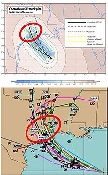
Top: Weather Research and Forecasting model simulation of Hurricane Rita tracks. Bottom: The spread of National Hurricane Center multi-model ensemble forecast.

Ensemble forecasting is a method used in or within numerical weather prediction. Instead of making a single forecast of the most likely weather, a set (or ensemble) of forecasts is produced. This set of forecasts aims to give an indication of the range of possible future states of the atmosphere. Ensemble forecasting is a form of Monte Carlo analysis. The multiple simulations are conducted to account for the two usual sources of uncertainty in forecast models: (1) the errors introduced by the use of imperfect initial conditions, amplified by the chaotic nature of the evolution equations of the atmosphere, which is often referred to as sensitive dependence on initial conditions; and (2) errors introduced because of imperfections in the model formulation, such as the approximate mathematical methods to solve the equations. Ideally, the verified future atmospheric state should fall within the predicted ensemble spread, and the amount of spread should be related to the uncertainty (error) of the forecast. In general, this approach can be used to make probabilistic forecasts of any dynamical system, and not just for weather prediction.

Instances

Today ensemble predictions are commonly made at most of the major operational weather prediction facilities worldwide, including:

Experimental ensemble forecasts are made at a number of universities, such as the University of Washington, and ensemble forecasts in the US are also generated by the US Navy and Air Force. There are various ways of viewing the data such as spaghetti plots, ensemble means or Postage Stamps where a number of different results from the models run can be compared.

History

As proposed by Edward Lorenz in 1963, it is impossible for long-range forecasts—those made more than two weeks in advance—to predict the state of the atmosphere with any degree of skill owing to the chaotic nature of the fluid dynamics equations involved. Furthermore, existing observation networks have limited spatial and temporal resolution (for example, over large bodies of water such as the Pacific Ocean), which introduces uncertainty into the true initial state of the atmosphere. While a set of equations, known as the Liouville equations, exists to determine the initial uncertainty in the model initialization, the equations are too complex to run in real-time, even with the use of supercomputers. The practical importance of ensemble forecasts derives from the fact that in a chaotic and hence nonlinear system, the rate of growth of forecast error is dependent on starting conditions. An ensemble forecast therefore provides a prior estimate of state-dependent predictability, i.e. an estimate of the types of weather that might occur, given inevitable uncertainties in the forecast initial conditions and in the accuracy of the computational representation of the equations. These uncertainties limit forecast model accuracy to about six days into the future. The first operational ensemble forecasts were produced for sub-seasonal timescales in 1985. However, it was realised that the philosophy underpinning such forecasts was also relevant on shorter timescales – timescales where predictions had previously been made by purely deterministic means.

Edward Epstein recognized in 1969 that the atmosphere could not be completely described with a single forecast run due to inherent uncertainty, and proposed a stochastic dynamic model that produced means and variances for the state of the atmosphere. Although these Monte Carlo simulations showed skill, in 1974 Cecil Leith revealed that they produced adequate forecasts only when the ensemble probability distribution was a representative sample of the probability distribution in the atmosphere. It was not until 1992 that ensemble forecasts began being prepared by the European Centre for Medium-Range Weather Forecasts (ECMWF) and the National Centers for Environmental Prediction (NCEP).

Methods for representing uncertainty

There are two main sources of uncertainty that must be accounted for when making an ensemble weather forecast: initial condition uncertainty and model uncertainty.

Initial condition uncertainty

Initial condition uncertainty arises due to errors in the estimate of the starting conditions for the forecast, both due to limited observations of the atmosphere, and uncertainties involved in using indirect measurements, such as satellite data, to measure the state of atmospheric variables. Initial condition uncertainty is represented by perturbing the starting conditions between the different ensemble members. This explores the range of starting conditions consistent with our knowledge of the current state of the atmosphere, together with its past evolution. There are a number of ways to generate these initial condition perturbations. The ECMWF model, the Ensemble Prediction System (EPS), uses a combination of singular vectors and an ensemble of data assimilations (EDA) to simulate the initial probability density. The singular vector perturbations are more active in the extra-tropics, while the EDA perturbations are more active in the tropics. The NCEP ensemble, the Global Ensemble Forecasting System, uses a technique known as vector breeding.

Model uncertainty

Model uncertainty arises due to the limitations of the forecast model. The process of representing the atmosphere in a computer model involves many simplifications such as the development of parametrisation schemes, which introduce errors into the forecast. Several techniques to represent model uncertainty have been proposed.

Perturbed parameter schemes

When developing a parametrisation scheme, many new parameters are introduced to represent simplified physical processes. These parameters may be very uncertain. For example, the 'entrainment coefficient' represents the turbulent mixing of dry environmental air into a convective cloud, and so represents a complex physical process using a single number. In a perturbed parameter approach, uncertain parameters in the model's parametrisation schemes are identified and their value changed between ensemble members. While in probabilistic climate modelling, such as climateprediction.net, these parameters are often held constant globally and throughout the integration, in modern numerical weather prediction it is more common to stochastically vary the value of the parameters in time and space. The degree of parameter perturbation can be guided using expert judgement, or by directly estimating the degree of parameter uncertainty for a given model.

Stochastic parametrisations

A traditional parametrisation scheme seeks to represent the average effect of the sub grid-scale motion (e.g. convective clouds) on the resolved scale state (e.g. the large scale temperature and wind fields). A stochastic parametrisation scheme recognises that there may be many sub-grid scale states consistent with a particular resolved scale state. Instead of predicting the most likely sub-grid scale motion, a stochastic parametrisation scheme represents one possible realisation of the sub-grid. It does this through including random numbers into the equations of motion. This samples from the probability distribution assigned to uncertain processes. Stochastic parametrisations have significantly improved the skill of weather forecasting models, and are now used in operational forecasting centres worldwide. Stochastic parametrisations were first developed at the European Centre for Medium Range Weather Forecasts.

Multi model ensembles

When many different forecast models are used to try to generate a forecast, the approach is termed multi-model ensemble forecasting. This method of forecasting can improve forecasts when compared to a single model-based approach. When the models within a multi-model ensemble are adjusted for their various biases, this process is known as "superensemble forecasting". This type of a forecast significantly reduces errors in model output. When models of different physical processes are combined, such as combinations of atmospheric, ocean and wave models, the multi-model ensemble is called hyper-ensemble.

Probability assessment

The ensemble forecast is usually evaluated by comparing the ensemble average of the individual forecasts for one forecast variable to the observed value of that variable (the "error"). This is combined with consideration of the degree of agreement between various forecasts within the ensemble system, as represented by their overall standard deviation or "spread". Ensemble spread can be visualised through tools such as spaghetti diagrams, which show the dispersion of one quantity on prognostic charts for specific time steps in the future. Another tool where ensemble spread is used is a meteogram, which shows the dispersion in the forecast of one quantity for one specific location. It is common for the ensemble spread to be too small, such that the observed atmospheric state falls outside of the ensemble forecast. This can lead the forecaster to be overconfident in their forecast. This problem becomes particularly severe for forecasts of the weather about 10 days in advance, particularly if model uncertainty is not accounted for in the forecast.

Reliability and resolution (calibration and sharpness)

The spread of the ensemble forecast indicates how confident the forecaster can be in his or her prediction. When ensemble spread is small and the forecast solutions are consistent within multiple model runs, forecasters perceive more confidence in the forecast in general. When the spread is large, this indicates more uncertainty in the prediction. Ideally, a spread-skill relationship should exist, whereby the spread of the ensemble is a good predictor of the expected error in the ensemble mean. If the forecast is reliable, the observed state will behave as if it is drawn from the forecast probability distribution. Reliability (or calibration) can be evaluated by comparing the standard deviation of the error in the ensemble mean with the forecast spread: for a reliable forecast, the two should match, both at different forecast lead times and for different locations.

The reliability of forecasts of a specific weather event can also be assessed. For example, if 30 of 50 members indicated greater than 1 cm rainfall during the next 24 h, the probability of exceeding 1 cm could be estimated to be 60%. The forecast would be considered reliable if, considering all the situations in the past when a 60% probability was forecast, on 60% of those occasions did the rainfall actually exceed 1 cm. In practice, the probabilities generated from operational weather ensemble forecasts are not highly reliable, though with a set of past forecasts (reforecasts or hindcasts) and observations, the probability estimates from the ensemble can be adjusted to ensure greater reliability.

Another desirable property of ensemble forecasts is resolution. This is an indication of how much the forecast deviates from the climatological event frequency – provided that the ensemble is reliable, increasing this deviation will increase the usefulness of the forecast. This forecast quality can also be considered in terms of sharpness, or how small the spread of the forecast is. The key aim of a forecaster should be to maximise sharpness, while maintaining reliability. Forecasts at long leads will inevitably not be particularly sharp (have particularly high resolution), for the inevitable (albeit usually small) errors in the initial condition will grow with increasing forecast lead until the expected difference between two model states is as large as the difference between two random states from the forecast model's climatology.

Calibration of ensemble forecasts

If ensemble forecasts are to be used for predicting probabilities of observed weather variables they typically need calibration in order to create unbiased and reliable forecasts. For forecasts of temperature one simple and effective method of calibration is linear regression, often known in this context as model output statistics. The linear regression model takes the ensemble mean as a predictor for the real temperature, ignores the distribution of ensemble members around the mean, and predicts probabilities using the distribution of residuals from the regression. In this calibration setup the value of the ensemble in improving the forecast is then that the ensemble mean typically gives a better forecast than any single ensemble member would, and not because of any information contained in the width or shape of the distribution of the members in the ensemble around the mean. However, in 2004, a generalisation of linear regression (now known as Nonhomogeneous Gaussian regression) was introduced that uses a linear transformation of the ensemble spread to give the width of the predictive distribution, and it was shown that this can lead to forecasts with higher skill than those based on linear regression alone. This proved for the first time that information in the shape of the distribution of the members of an ensemble around the mean, in this case summarized by the ensemble spread, can be used to improve forecasts relative to linear regression. Whether or not linear regression can be beaten by using the ensemble spread in this way varies, depending on the forecast system, forecast variable and lead time.

Predicting the size of forecast changes

In addition to being used to improve predictions of uncertainty, the ensemble spread can also be used as a predictor for the likely size of changes in the mean forecast from one forecast to the next. This works because, in some ensemble forecast systems, narrow ensembles tend to precede small changes in the mean, while wide ensembles tend to precede larger changes in the mean. This has applications in the trading industries, for whom understanding the likely sizes of future forecast changes can be important.

Co-ordinated research

The Observing System Research and Predictability Experiment (THORPEX) is a 10-year international research and development programme to accelerate improvements in the accuracy of one-day to two-week high impact weather forecasts for the benefit of society, the economy and the environment. It establishes an organizational framework that addresses weather research and forecast problems whose solutions will be accelerated through international collaboration among academic institutions, operational forecast centres and users of forecast products.

One of its key components is THORPEX Interactive Grand Global Ensemble (TIGGE), a World Weather Research Programme to accelerate the improvements in the accuracy of 1-day to 2 week high-impact weather forecasts for the benefit of humanity. Centralized archives of ensemble model forecast data, from many international centers, are used to enable extensive data sharing and research.

Human fertilization

From Wikipedia, the free encyclopedia
 
Human fertilization
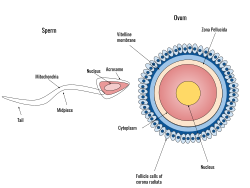
Sperm about to enter the ovum with acrosomal head ready to penetrate the zona pellucida and fertilize the egg
 
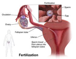
Illustration depicting ovulation and fertilization

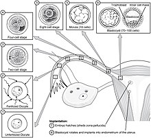
Human fertilization is the union of a human egg and sperm, occurring primarily in the ampulla of the fallopian tube. The result of this union leads to the production of a fertilized egg called a zygote, initiating embryonic development. Scientists discovered the dynamics of human fertilization in the nineteenth century.

The process of fertilization involves a sperm fusing with an ovum. The most common sequence begins with ejaculation during copulation, follows with ovulation, and finishes with fertilization. Various exceptions to this sequence are possible, including artificial insemination, in vitro fertilization, external ejaculation without copulation, or copulation shortly after ovulation. Upon encountering the secondary oocyte, the acrosome of the sperm produces enzymes which allow it to burrow through the outer shell called the zona pellucida of the egg. The sperm plasma then fuses with the egg's plasma membrane and their nuclei fuse, triggering the sperm head to disconnect from its flagellum as the egg travels down the fallopian tube to reach the uterus.

In vitro fertilization (IVF) is a process by which egg cells are fertilized by sperm outside the womb, in vitro.

History

In Antiquity, Aristotle depicted the formation of new individuals occurring through fusion of male and female fluids, with form and function emerging gradually, in a mode called by him as epigenetic. He proposed that during conception the female supplied the material, or the body, while the male provided the soul.

Galen argued that during conception the male and the female both produced a seed. However, the male seed was thicker and more powerful than the female seed because it had a natural heat that the female seed lacked.

Hippocrates theorized that fertilization occurred when the male and female seed came together, and the sex of the child would be determined by the strength of the seed. If both parents had strong seed, the child would be male. If both parents had weak seed the child would be female. If one parent produced strong seed and the other produced weak seed, the more numerous type of sperm would determine the sex. Hippocrates did not assign the production of strong or weak seed to a specific sex; both males and females could produce strong or weak seed.

Sperm and oocyte meet

Ampulla

Fertilization occurs in the ampulla of the fallopian tube, the section that curves around the ovary. Capacitated sperm are attracted to progesterone, which is secreted from the cumulus cells surrounding the oocyte. Progesterone binds to the CatSper receptor on the sperm membrane and increases intracellular calcium levels, causing hyperactive motility. The sperm will continue to swim towards higher concentrations of progesterone, effectively guiding it to the oocyte. Around 200 of 200 millions spermatozoa reach the ampulla.

Sperm preparation

The sperm entering the ovum using acrosomal enzymes to dissolve the gelatinous envelope (zona pellucida)of the oocyte.

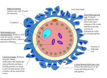
At the beginning of the process, the sperm undergoes a series of changes, as freshly ejaculated sperm is unable or poorly able to fertilize. The sperm must undergo capacitation in the female's reproductive tract, which increases its motility and hyperpolarizes its membrane, preparing it for the acrosome reaction, the enzymatic penetration of the egg's tough membrane, the zona pellucida, which surrounds the oocyte.

Corona radiata

The sperm binds through the corona radiata, a layer of follicle cells on the outside of the secondary oocyte. The corona radiata sends out chemicals that attract the sperm in the fallopian tube to the oocyte. It lies above the zona pellucida, a membrane of glycoproteins that surrounds the oocyte. 

Cone of attraction and perivitelline membrane

Where the spermatozoan is about to pierce, the yolk (ooplasm) is drawn out into a conical elevation, termed the cone of attraction or reception cone. Once the spermatozoon has entered, the peripheral portion of the yolk changes into a membrane, the perivitelline membrane, which prevents the passage of additional spermatozoa.

Zona pellucida and acrosome reaction

After binding to the corona radiata the sperm reaches the zona pellucida, which is an extracellular matrix of glycoproteins. A ZP3 glycoprotein on the zona pellucida binds to a receptor on the cell surface of the sperm head. This binding triggers the acrosome to burst, releasing acrosomal enzymes that help the sperm penetrate through the thick zona pellucida layer surrounding the oocyte, ultimately gaining access to the egg's cell membrane.

Some sperm cells consume their acrosome prematurely on the surface of the egg cell, facilitating the penetration by other sperm cells. As a population, mature haploid sperm cells have on average 50% genome similarity, so the premature acrosomal reactions aid fertilization by a member of the same cohort. It may be regarded as a mechanism of kin selection.

Recent studies have shown that the egg is not passive during this process. In other words, they too appear to undergo changes that help facilitate such interaction.

Fusion

Fertilization and implantation in humans.

Cortical reaction

After the sperm enters the cytoplasm of the oocyte, the tail and the outer coating of the sperm disintegrate. The fusion of sperm and oocyte membranes causes cortical reaction to occur. Cortical granules inside the secondary oocyte fuse with the plasma membrane of the cell, causing enzymes inside these granules to be expelled by exocytosis to the zona pellucida. This in turn causes the glycoproteins in the zona pellucida to cross-link with each other — i.e. the enzymes cause the ZP2 to hydrolyse into ZP2f — making the whole matrix hard and impermeable to sperm. This prevents fertilization of an egg by more than one sperm.

Fusion of genetic material

Preparation

In preparation for the fusion of their genetic material both the oocyte and the sperm undergo transformations as a reaction to the fusion of cell membranes.

The oocyte completes its second meiotic division. This results in a mature haploid ovum and the release of a polar body. The nucleus of the oocyte is called a pronucleus in this process, to distinguish it from the nuclei that are the result of fertilization.

Drawing of an ovum

The sperm's tail and mitochondria degenerate with the formation of the male pronucleus. This is why all mitochondria in humans are of maternal origin. Still, a considerable amount of RNA from the sperm is delivered to the resulting embryo and likely influences embryo development and the phenotype of the offspring.

Fusion

The sperm nucleus then fuses with the ovum, enabling fusion of their genetic material.

Blocks of polyspermy

When the sperm enters the perivitelline space, a sperm-specific protein Izumo on the head binds to Juno receptors on the oocyte membrane. Once it’s bound, two blocks to polyspermy then occur. After approximately 40 minutes, the other Juno receptors on the oocyte are lost from the membrane, causing it to no longer be fusogenic. Additionally, the cortical reaction will happen which is caused by ovastacin binding and cleaving ZP2 receptors on the zona pellucida. These two blocks of polyspermy are what prevent the zygote from having too much DNA.

Replication

The pronuclei migrate toward the center of the oocyte, rapidly replicating their DNA as they do so to prepare the zygote for its first mitotic division.

Mitosis

Usually 23 chromosomes from spermatozoon and 23 chromosomes from egg cell fuse (approximately half of spermatozoons carry X chromosome and the other half Y chromosome). Their membranes dissolve, leaving no barriers between the male and female chromosomes. During this dissolution, a mitotic spindle forms between them. The spindle captures the chromosomes before they disperse in the egg cytoplasm. Upon subsequently undergoing mitosis (which includes pulling of chromatids towards centrioles in anaphase) the cell gathers genetic material from the male and female together. Thus, the first mitosis of the union of sperm and oocyte is the actual fusion of their chromosomes.

Each of the two daughter cells resulting from that mitosis has one replica of each chromatid that was replicated in the previous stage. Thus, they are genetically identical.

Fertilization age

Fertilization is the event most commonly used to mark the beginning point of life, in descriptions of prenatal development of the embryo or fetus. The resultant age is known as fertilization age, fertilizational age, conceptional age, embryonic age, fetal age or (intrauterine) developmental (IUD) age.

Gestational age, in contrast, takes the beginning of the last menstrual period (LMP) as the start point. By convention, gestational age is calculated by adding 14 days to fertilization age and vice versa. Fertilization though usually occurs within a day of ovulation, which, in turn, occurs on average 14.6 days after the beginning of the preceding menstruation (LMP). There is also considerable variability in this interval, with a 95% prediction interval of the ovulation of 9 to 20 days after menstruation even for an average woman who has a mean LMP-to-ovulation time of 14.6. In a reference group representing all women, the 95% prediction interval of the LMP-to-ovulation is 8.2 to 20.5 days.

The average time to birth has been estimated to be 268 days (38 weeks and two days) from ovulation, with a standard deviation of 10 days or coefficient of variation of 3.7%.

Fertilization age is sometimes used postnatally (after birth) as well to estimate various risk factors. For example, it is a better predictor than postnatal age for risk of intraventricular hemorrhage in premature babies treated with extracorporeal membrane oxygenation.

Diseases affecting human fertility

Various disorders can arise from defects in the fertilization process. Whether that results in the process of contact between the sperm and egg, or the state of health of the biological parent carrying the zygote cell. The following are a few of the diseases that can occur and be present during the process.

  • Polyspermy results from multiple sperm fertilizing an egg, leading to an offset number of chromosomes within the embryo. Polyspermy, while physiologically possible in some species of vertebrates and invertebrates, is a lethal condition for the human zygote.
  • Polycystic ovary syndrome is a condition in which the woman does not produce enough follicle stimulating hormone and excessively produces androgens. This results in the ovulation period between contact of the egg being postponed or excluded.
  • Autoimmune disorders can lead to complications in implantation of the egg in the uterus, which may be the immune system’s attack response to an established embryo on the uterine wall.
  • Cancer ultimately affects fertility and may lead to birth defects or miscarriages. Cancer severely damages reproductive organs, which affects fertility. 
  • Endocrine system disorders affect human fertility by decreasing the body’s ability to produce the level of hormones needed to successfully carry a zygote. Examples of these disorders include diabetes, adrenal disorders, and thyroid disorders.
  • Endometriosis is a condition that affects women in which the tissue normally produced in the uterus proceeds to grow outside of the uterus. This leads to extreme amounts of pain and discomfort and may result in an irregular menstrual cycle.

Bayesian inference

From Wikipedia, the free encyclopedia https://en.wikipedia.org/wiki/Bayesian_inference Bayesian inference ( / ...